


Abstract
Under physiological and pathological conditions, cells experience large forces and deformations that often exceed the linear viscoelastic regime. Here we drive CD34+ cells isolated from healthy and leukemic bone marrows in the highly nonlinear elasto-plastic regime, by poking their perinuclear region with a sharp AFM cantilever tip. We use the wavelet transform mathematical microscope to identify singular events in the force-indentation curves induced by local rupture events in the cytoskeleton (CSK). We distinguish two types of rupture events, brittle failures likely corresponding to irreversible ruptures in a stiff and highly cross-linked CSK and ductile failures resulting from dynamic cross-linker unbindings during plastic deformation without loss of CSK integrity. We propose a stochastic multiplicative cascade model of mechanical ruptures that reproduces quantitatively the experimental distributions of the energy released during these events, and provides some mathematical and mechanistic understanding of the robustness of the log-normal statistics observed in both brittle and ductile situations. We also show that brittle failures are relatively more prominent in leukemia than in healthy cells suggesting their greater fragility.
Export citation and abstract BibTeX RIS

Original content from this work may be used under the terms of the Creative Commons Attribution 3.0 licence. Any further distribution of this work must maintain attribution to the author(s) and the title of the work, journal citation and DOI.
1. Introduction
As the elementary building block of living systems, cells are active mechanical machines that constantly remodel their structural organization to withstand forces and deformations and to promptly adapt to their mechanical environment [1, 2]. This versatility is fundamentally required for many vital cellular functions, and an alteration of the cell mechanical properties can participate in pathogenesis and disease progression [3, 4]. Identifying under which conditions is the mechanical resilience of living cells compromised is therefore a critical issue. Significant progress in the past decades has provided a rather complete picture of the linear mechanical response to small applied stresses or strains [5–11]. However, cells are often subject to large deformations and reach nonlinear regimes that are far from being well understood [8, 9, 12–14]. The fascinating mechanical properties of living cells are mediated by the cytoskeleton (CSK), a dynamic network of filamentous proteins composed of actin filaments, microtubules, and intermediate filaments [7–9, 15–17]. The actin filaments are cross-linked by a wide variety of actin binding proteins (ABPs) [7–9, 12, 15–18]. By tuning the proportions of passive and active ABPs, living cells can control their power-law (scale-free) CSK rheology [7, 19]. Interestingly, cells exhibit both solid and liquid-like properties. Solid-like behavior is associated with strongly cross-linked actin filaments which resist sliding and accumulate tension (fimbrin and fascin are compact cross-linking proteins that create parallel-aligned actin networks (actin bundles) and are found in stiffer membrane protusions of filopodia [20, 21]). In contrast, weakly cross-linking proteins produce actin filaments which slide more readily, enabling the network to flow as a liquid (α-actinin and filamin-A are less compact and form networks with more widely spaced and orthogonally aligned actin filaments[22]). All these actin cross-linking and/or bundling proteins work cooperatively or competitively, for instance fascin and α-actinin were recently shown to segregate into discrete bundled domains that are specifically recognized by other ABPs [23]. Under nonlinear loading conditions, living cells can display apparently opposite behaviors ranging from stress stiffening mainly governed by filament and/or cross-linker nonlinear elasticity [8, 9, 12, 13], to stretch softening and fluidization likely due to force-induced unbinding of ABPs [8, 9, 14]. This paradox can be solved by considering that, upon large deformations, the CSK of a living cell can undergo deep structural transformations such as the unfolding of protein domains, the unbinding of cytoskeletal cross-linkers, and the breaking of weak sacrificial bonds. All these structural changes are inelastic (non-reversible in a strict sense), they dissipate locally the elastic energy of the CSK network (structural damping) [24, 25]. Unbinding events and bond breakings confer living cells with the unique ability to adapt to different mechanical situations by actively controlling the amount of stress stiffening and fluidization [24, 26]. At the same time, such events reduce the connectivity of the CSK and may result in permanent plastic deformations or even more dramatic irreversible failures [8, 9] which, for instance, could be at the origin of the recently observed incomplete shape recovery of living cells after repeated creep [27]. These effects are reminiscent of those in cyclically loaded solids which can lead to fatigue-induced failure [28–30].
In this paper, we use a nanoindentation (AFM) technique [31–35] to experimentally investigate the nonlinear mechanical plasticity of single immature CD34+ hematopoietic cells from healthy donors and patients suffering from chronic myelogenous leukemia (CML) in chronic phase (CP) harvested at diagnosis [36]. Classical analysis of force-indentation curves (FICs) aims at estimating an elastic modulus by fitting the curves with linear elastic models [37, 38]. Here, in contrast, we engineer a wavelet-based multi-scale method [36, 39] to identify singularities in the FICs that likely correspond to rupture events in the CSK. Our study provides compelling evidence of the existence of two distinct populations of avalanche rupture events, that we identify to ductile (corresponding to weakly cross-linked filaments) and brittle (corresponding to tightly cross-linked filaments) failures. Both mechanisms display fat-tail distributions of released energy well approximated by log-normal distributions. This is surprising given the ubiquity of power-law statistics for avalanches in solids [28–30]. We develop a minimal model that reproduces quantitatively the experimental released energy distributions, and provides some mechanistic interpretation of both the ductile and brittle rupture regimes. Despite this phenomenological model does not take into account the visco-elasticity of individual polymer chains constituting the CSK filaments, it sheds a new light on the local unbinding events as a major mechanism underlying the nonlinear response of living cells to large deformations and it further shows that brittle failures are more frequent in CML cells as the signature of their higher mechanical fragility.
2. Results
2.1. Nanoindentation of living hematopoietic primary cells
CML arises from a hematopoietic stem cell transformation following the formation of the BCR-ABL oncogene by a single reciprocal chromosomal translocation t(9;22) [40]. In CML, BCR-ABL+ cells of the myeloid lineage proliferate uncontrollably, the bone marrow density increases considerably, and their mechanical properties change during disease progression [41]. In transformed cells [42], BCR-ABL was shown to bind actin filaments, to inhibit their polymerization and to disorganize the CSK into punctuate, juxtanuclear aggregates [43–45]. We used AFM to indent single hematopoietic purified CD34+ cells from CP-CML patients at diagnosis and healthy donor bone marrows [36] (see appendix A). We indented the cells by moving vertically the AFM cantilever (figure 1(a)) toward their perinuclear central region (figure 1(b)), at constant speed V0 = 1 μm s−1 until a cantilever set-point force was reached. Then the cantilever was withdrawn from the sample at the same constant speed (−V0) back to its starting position (figures 1(c) and (d)). From these indentation experiments, the cell shear relaxation modulus G(Z) was estimated as the second-order derivative of the FIC (see equation (B13) in appendix B) [36, 39]. From the approach and retract FICs, the initial Gi and global Gg shear moduli, and the dissipation loss Dl were retrieved (see figure S1 is available online at stacks.iop.org/NJP/20/053057/mmedia and supplemental material11 ). When these FICs do not superimpose (figures 1(c) and (d)), Dl quantifies the percentage of work not restituted during retract and dissipated partly as viscous loss [31, 36]. Interestingly, the experimental FICs display fluctuations that locally exceed the background thermal fluctuations of the AFM cantilever [36] (figures 1(c) and (d)). We developed a wavelet-based detection method of these singular events that amounts to detect local curvature minima Gm and maxima GM in the FICs (figures 1(e) and (f)) (see also appendix B, and figures S2 and S3 (see footnote 11)). For each disruption event, we computed the force drop ΔF, the penetration length ΔZ, and the released energy E = ΔF.ΔZ (figure 1(e)). FICs without disruption events were not included in the statistics.

Figure 1. Principle of living cell indentation and detection of rupture events with an AFM cantilever tip. (a) Sketch of the AFM set up. (b) Microscopy transmission image of the perinuclear central region of an hematopoietic cell probed by the cantilever tip. Scale bar: 10 μm. (c) Typical approach (red) and retract (green) FICs collected on a CML hematopoietic cell (CP-CML patient). (d) Same as (c) but for a normal hematopoietic cell (healthy donor). (e) Zoom on (c) around a disruption event. (f) Corresponding second-order derivative G(Z) of the FIC (see equation (B13) in appendix B) computed with a wavelet of size  ; the local minima Gm (resp. maxima GM) of
  corresponding to a strong negative (resp. positive) curvature of the FIC are marked with black triangles (resp. dots). In a close neighborhood of Gm and GM, the local maxima and minima of the FIC are detected and marked with blue triangles and dots in (c) and (e). The force drop ΔF of a disruption event is corrected by taking into account the increasing behavior of the FIC (linear dashed–dotted line in (e)).
Download figure:
Standard image High-resolution image2.2. Ductile versus brittle rupture events
We collected two large sets of single cell FICs from 5 CP-CML patients (1301 FICs—49 cells) and 5 healthy donors (1671 FICs—60 cells). We detected 6161 singular rupture events distributed on 1153 FICs in CP-CML cells as compared to 6765 rupture events distributed on 1111 FICs in normal cells. Thus only 11.4% (148/1301) of FICs do not display rupture events for CML cells which is significantly lower than 33.5% (560/1671) for normal cells. The computation of the normalized histograms (p.d.f. for probability density function) of  , ΔF, and E of these rupture events, revealed rather wide distributions with fat-tail (see figure S4 (see footnote 11)). When focusing on ΔZ (nm), which can also be interpreted as the time duration Δt = ΔZ/V0 (ms) of the rupture event, we got very satisfactory fits of the p.d.f. of
  with the sum of two distinct Gaussian distributions (see equation (B14) in appendix B) for both normal and CML cells (figures 2(a) and (b)). Thus, we identified two populations of rupture events, a subpopulation 1 of rather short duration (
 ) and weakly penetrating (
 ) failures, and a subpopulation 2 of longer (
 ) and deeply penetrating (
 ) failures. But what distinguishes CML from normal cells is the higher percentage (α = 0.34 compared to 0.26) of the larger rupture events (subpopulation 2) in the CP-CML cells, as an indication of their greater mechanical brittleness.
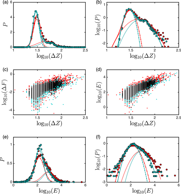
Figure 2. Statistical analysis of the indentation depths (nm), force drops (nN) and released energies (kBT) of disruption events. These parameters were obtained from local disruption events collected from the FICs of the two sets of CML (red) and normal (blue) cells. (a) Normalized histograms of  the dots represent the experimental data and the continuous lines the corresponding fits by the sum of 2 Gaussian distributions (see equation (B14) in appendix B) with parameters α = 0.34, and μ1 = 1.49, σ1 = 0.07 corresponding to the following means
  and
and  (red dotted–dashed line), μ2 = 1.67, σ2 = 0.18, i.e.,
  and
and  (red dotted line) for CML cells, and α = 0.26, and μ1 = 1.47, σ1 = 0.06, i.e.,
  and
and  (blue dotted–dashed line), μ2 = 1.70, σ2 = 0.15, i.e.,
  , and
, and  (blue dotted line) for normal cells. (b) Same as (a) but in a logarithmic representation where Gaussians become parabolae. (c) Scatter plot of
  versus
  each red (resp. blue) dot corresponds to a rupture event in a CML (resp. normal) FIC; whenever a red dot and a blue dot superimpose they were turned into black. (d) Scatter plot of
  versus
  . (e) Normalized histograms of
  same representation as for
  in (a); the parameters of the fit with the sum of 2 Gaussian distributions are for CML cells: α = 0.34 and μ1 = 2.15, σ1 = 0.40, μ2 = 2.89, σ2 = 0.51, and for healthy cells: α = 0.26, and μ1 = 2.14, σ1 = 0.34, μ2 = 2.87, σ2 = 0.41 (table 1). (f) Same as (e) but in a logarithmic representation.
Download figure:
Standard image High-resolution imageWhen investigating the correlations between ΔZ, ΔF and E, we found a rather strong correlation between  and
and  for both the CML (Pearson's correlation coefficient r = 0.68) and the normal (r = 0.62) cells. Log10 (E) and
  were also found significantly correlated in CML (r = 0.83) and in normal (r = 0.80) cells. These correlations issue from the existence of two clouds of points in the respective scatter plots (figures 2(c) and (d)), corresponding to subpopulation 1 of small indentation depth, short duration, small force drop and low released energy failures, and to subpopulation 2 of large indentation depth, long duration, large force drop and high released energy failures. We will classify the former as ductile and the latter as brittle rupture events.
2.3. Log-normal statistics of released energy during rupture events
The pertinence of the fitting of the p.d.f. of  (figure 2(e)) by the sum of 2 Gaussians is compelling when using a logarithmic representation (figure 2(f)). For the CML cells, when fixing the relative percentages of ductile (1 − α = 0.66) and brittle (α = 0.34) rupture events as previously estimated, we obtained the parameter values reported in table 1 with the following arithmetic and geometric means
  kBT (resp.
  kBT), and
  kBT (resp.
  kBT). For normal cells, when fixing α = 0.26 (1 − α = 0.74), we ended with consistent parameter values (table 1) with
  kBT (resp.
  kBT), and
  kBT (resp.
  kBT). Note that the standard deviations of the Gaussian distributions for
  are slightly larger for CML than for normal cells and this for both ductile and brittle events.
Table 1.
Distributions of energy released during ductile and brittle rupture events in normal and CML cells: simulations versus experiments. Characteristics ( , σN,
, σN,  ,
,  ,
,  ,
,  ) of the numerical cascades simulated with equation (2) for parameters values a0,
  , ΔE0 = 12 kBT,
  kBT versus experimental data (figures 2(e) and 2(f)).
| Normal Cells | CML Cells | |
|---|---|---|
| Ductile | ||
| Model parameters | a0 = 1.3,  , Δa = 0.39 , Δa = 0.39 |
a0 = 1.3,  , Δa = 0.48 , Δa = 0.48 |
| Simulations |
 , σN = 3 , σN = 3 |
 , σN = 4 , σN = 4 |
| μ1 = 2.17, σ1 = 0.31 | μ1 = 2.13, σ1 = 0.38 | |
 kBT, kBT,  kBT kBT |
 kBT, kBT,  kBT kBT |
|
| Experiments | μ1 = 2.14, σ1 = 0.34 | μ1 = 2.15, σ1 = 0.40 |
 kBT, kBT,  kBT kBT |
 kBT, kBT,  kBT kBT |
|
| Brittle | ||
| Model parameters | a0 = 1.3,  , Δa = 0.35 , Δa = 0.35 |
a0 = 1.3,  , Δa = 0.38 , Δa = 0.38 |
| Simulations |
 , σN = 7 , σN = 7 |
 , σN = 8 , σN = 8 |
| μ2 = 2.84, σ2 = 0.42 | μ2 = 2.92, σ2 = 0.47 | |
 kBT, kBT,  kBT kBT |
 kBT, kBT,  kBT kBT |
|
| Experiments | μ2 = 2.87, σ2 = 0.41 | μ2 = 2.89, σ2 = 0.51 |
 kBT, kBT,  kBT kBT |
 kBT, kBT,  kBT kBT |
|
When comparing the mean released energies during ductile (∼200 kBT) and brittle (∼1300 kBT) rupture events to the dissociation energies of α-actinin/actin binding (∼4.3 kBT) and of filamin/actin binding (∼3.6 kBT) [46], we obtain rough estimates for the number of ABP unbindings during ductile (∼50) and brittle (∼325) rupture events. Thus, more than 6 times energy is released during brittle failures that last (∼50 ms) not more than twice the duration (∼30 ms) of ductile failures, meaning that the mean rate of released energy is significantly higher during brittle failures. Interestingly, the computation of the global Gg and initial Gi shear moduli (see figure S1 (see footnote 11)) confirms that CML cells are stiffer ( kPa,
kPa,  kPa) than normal ones (
 kPa,
kPa,  kPa) [36]. In particular, about 37% of FICs bear mean shear relaxation moduli (Gg) larger than 1 kPa in CML cells with very low (7%) counter part in normal cells (see figure S5 (see footnote 11)). Altogether, these observations show that CML cells display a significant proportion of highly tensed perinuclear zones propitious to localized brittle failures by disruption of cross-linked CSK domains impeding complete shape recovery after deformation. This interpretation is strengthened by the experimental observation of an important structural alteration of the actin CSK of immature TF1 cells consecutive to BCR-ABL oncogene transduction. In particular, confocal fluorescence microscopy revealed that in this model of human CML [40–45], juxtanuclear actin aggregates were found in almost 30% of the BCR-ABL-transduced TF1 cells at the expense of the cortical F-actin [43, 45] (figure 3(b)). Very likely, these solid structures were induced by the oncogene since they were rarely observed in the parental TF1 cell line (figure 3(a)).
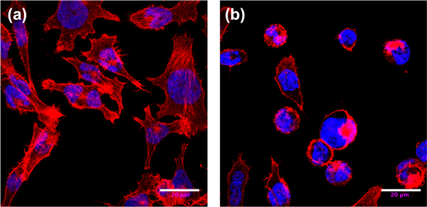
Figure 3. Cytoskeleton structure of TF1 cells revealed by confocal microscopy. (a) Parental TF1 cells. (b) TF1 hematopoietic cells after transfection by the CML BCR-ABL oncogene. F-actin was labeled with phalloidin-rhodamin (red), and the nuclei were labeled with DAPI (blue). Immunofluorescence images were taken using a confocal microscope on fixed TF1 and TF1-BCR-ABL adherent cells on fibronectin (see appendix A). Scale bar: 20 μm.
Download figure:
Standard image High-resolution image3. Computational model
To account for the observed log-normal released energy distributions (figures 2(e) and (f)), we propose a multiplicative cascade description of CSK failure events that is inspired from pioneering works on population growth dynamics [47–49].
3.1. Fat tail probability distribution functions: log-normal versus power-law distributions
P.d.f.s with heavy tails have been widely observed in various domains of fundamental and applied sciences [50]. The most popular fat-tail distributions are power-law and log-normal distributions that often have been considered as competing models of experimental data [48, 49]. Power-law distributions are commonly thought to be a statistical characteristics of systems that display space and/or time scale invariance properties [50] with as notable examples scale-free networks [51] and self-organized critical systems [52–54]. Log-normal distributions are paradigmatic fat-tail distributions generated by self-similar fragmentation and more generally multiplicative processes [55, 56] with as historical example the energy cascade model of fully developed turbulence [57]. But, as originally proposed by Kesten [47], power-law and log-normal distributions are indeed intrinsically connected when combining multiplicative and additive random processes:

where St is the size of a population at time t, at the random positive growth factor, and bt a small positive random increment. In the absence of the additive bt term, one recovers the multiplicative Gibrat's law [58] of proportional growth which is nothing but a random walk in log-size leading to a log-normal distribution of St. But this distribution is not stable since when the time increases the process St either asymptotically shrinks stochastically to zero ( ) or diverges to infinity (
 ). Kesten [47] showed that provided (
 ), adding the random variable bt prevents the divergence of the log-normal distribution of St which progressively switches and converges to a stationary power-law distribution with exponent α given by the strictly positive solution of the equation
  .
.
3.2. A log-normal released energy cascade model
Our model of CSK cascading rupture events is deliberately reductionist with a minimal number of parameters. At the cascade step n + 1, the energy released ΔEn+1 satisfies a Gibrat's multiplicative law [58], meaning that it can be expressed as a percentage of the energy ΔEn released at the previous cascade step:

where an is a Gaussian random variable with initial value a0 > 1, whose mean  decreases exponentially (CSK structural relaxation) with a characteristic depth
  and a fixed standard deviation
  . Note that the relationship between the cascade index n and time is not defined in our model since there is no reason a priori to assume that the CSK rupture cascade steps occur at regular time intervals. Starting from some initiation threshold ΔE0, ΔEn will asymptotically tend to zero because of the exponentially decreasing multiplicative constant an which will become smaller than 1 after some finite number of steps. The cascade will end when
  , where
  is a cascade arrest energy cut-off. During the N steps of the CSK rupture cascade, the total released energy is:

Our random cascade model mainly depends on three parameters: a0,  and Δa. N is a random variable that depends on the realization of the cascade. Its p.d.f. P(N) is well approximated by a Gaussian distribution (figure 4). To account for the experimental data, all our simulations of the released energy cascade model defined by equation (2) were performed for rather small values of Δa ≪ 1. In this limit, E (equation (3)) can be approximated by:

From the well known identity  , we get

Thus a good approximation of the mean of E can be obtained by replacing N by the nearest integer ![$[\overline{N}]$](https://content.cld.iop.org/journals/1367-2630/20/5/053057/revision2/njpaac3c7ieqn83.gif) of its mean
of its mean  in equation (5):

We recall that the p.d.f. of the random variable N was shown to be well approximated by a Gaussian (figure 4). Now from the Taylor expansion of  at first order, we can show by taking the ensemble average on both sides of this equation that
  is well approximated by

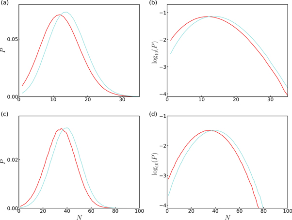
Figure 4. Distributions of the number of steps N of the log-normal rupture cascade model. P.d.f. of N computed from 1.2 × 10⁶ realizations of the multiplicative process defined by equation (2), for parameters values given in table S1 (see footnote 11). (a) Ductile rupture events in normal (blue) and CML (red) cells. (b) Semi-log representation. (c) Brittle rupture events in normal (blue) and CML (red) cells. (d) Semi-log representation.
Download figure:
Standard image High-resolution imageWe have confirmed numerically the pertinence of this approximation in all our simulations with a rather good accuracy (<5% error). Now, if we assume that the energy cascade ends when the difference between  and the threshold ΔE* is of the order of Δa, i.e.
  , then

where K is a constant that has been numerically estimated of order 1 (e.g. K = 1.52 ± 0.05 for a0 = 1.3,  and Δa = 0.36, see figure 5). Equation (8) shows that the mean size
  of the energy cascade increases as expected when increasing a0 and
  , but decreases when increasing Δa, since the probability to have a
  after a limited number n of cascade steps increases (see figure S6 (see footnote 11)).
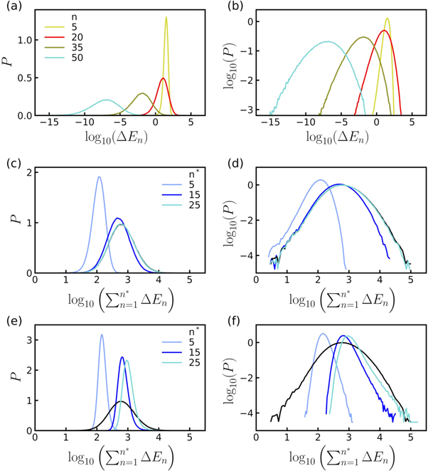
Figure 5. Released energy (kBT) distributions simulated with the log-normal rupture cascade model. (a) P.d.f. of  computed from 1.2 × 10⁶ realizations of the multiplicative process defined by equation (2), for parameters values: a0 = 1.3,
  , Δa = 0.36, ΔE0 = 12 kBT and ΔE* = 0. The colors correspond to n = 5 (yellow), 20 (red), 35 (dark green), 50 (cyan); P(E) (black) is shown for comparison. (b) Same as (a) but in a logarithmic representation. (c) P.d.f. of
  , where
  for n* = 5 (light blue), 15 (dark blue), 25 (cyan) and N (black). (d) Same as (c) but in a logarithmic representation. (e) Same as (c) but for surrogate uncorrelated released energy cascades (see text). (f) Same as (e) but in a logarithmic representation. In (e) and (f),
  (black) has the same meaning as in (c) and (d) respectively.
Download figure:
Standard image High-resolution image3.3. Theoretical considerations based on Beaulieu's mathematical results
In our simulations, we fixed a0 = 1.3 and started iterating equation (2) with the initial threshold ΔE0 = 12 kBT. Note that ΔE0 is a multiplicative factor that only shifts the p.d.f. of  without affecting its shape. When using the cut-off
  (
( ), after some transient (n ≳ 5), the p.d.f. of ΔEn obtained from 1.2 × 10⁶ realizations with parameter values
  and Δa = 0.36 is well approximated by a log-normal Gibrat's law [58], as expected from multiplicative process (figures 5(a) and (b)). What is more surprising is the fact that the sum E of these log-normal variables turns out also to be well approximated by a log-normal distribution and not by a normal distribution as expected from the central limit theorem. Indeed, this theorem does not apply since the random variables ΔEn are not only not identically distributed but correlated. Beaulieu [59] has recently proved an extended log-normal limit theorem that states that the limit distribution of the sum of nonidentically distributed correlated log-normal random variables is a log-normal distribution. When investigating how the energy
  , released during the first n* steps of the cascade converges to the total released energy EN, we confirmed a rather fast convergence to an asymptotic log-normal distribution (figures 5(c) and (d)). When numerically simulating surrogated uncorrelated released energy cascades where at each step, ΔEn is randomly generated with the p.d.f. P(ΔEn) (figure 5(a)) but independently of the previous cascade steps, then the sum
  no longer converges to a log-normal distribution but to a normal distribution as expected for uncorrelated random variables (figures 5(e) and (f)). This theoretical argument suggests that the log-normal distribution observed experimentally (figures 2(e) and (f)) are evidence that the different cascade steps of ABP unbinding are correlated. This theoretical understanding applies to all the numerical simulations reported in this study, for ductile and brittle rupture events, in normal as well as in CML cells (table 1, figures 6 and 7).

Figure 6. Computed model simulations of the p.d.fs P(E) of energy (kBT) released during rupture events in normal (blue) and CML (red) cells. Ductile rupture events: (a) semi-log representation; (b) log–log representation. Brittle rupture events: (c) semi-log representation; (d) log–log representation. All rupture events: (e) semi-log representation; (f) log–log representation. The triangles (△) represent the experimental data (figures 2(e) and (f)); ductile and brittle rupture event log-normal p.d.fs were disentangled using a classical two component Gaussian mixture model (see appendix B). The curves represent the prediction of the released energy cascade model defined by equation (2); the corresponding sets of model parameters are given in table 1.
Download figure:
Standard image High-resolution image
Figure 7. Model predictions for the energy released rate per cascade step (kBT/step). (a)  versus n. (b)
  versus n/N. The continuous (resp. dotted–dashed) lines correspond to brittle (resp. ductile) rupture events. The colors correspond to normal (blue) and CML (red) cells. The corresponding sets of model parameters are given in table 1.
Download figure:
Standard image High-resolution image
3.4. Mechanistic interpretation of ductile and brittle rupture events
We performed numerical simulations of the released energy cascade model to reproduce quantitatively the p.d.fs of E obtained for both normal and CML cells (figures 2(e) and (f)) (see appendix C). To this end, the p.d.f.s corresponding to ductile and brittle rupture events were disentangled with a two component Gaussian mixture model (see appendix B). When fixing ΔE0 = 12 kBT and ΔE* = 4 kBT (characteristic unbinding energy of ABPs [46]), sets of parameters (a0,  , Δa) values (table 1) were found providing quite satisfactory fits of the experimental released energy distributions (figure 6). For ductile rupture events, the mean number of cascade steps is rather limited for normal (
 ) as well as CML (
 ) cells and correspond to low mean released energy values
  and likely to a few tens of ABP unbindings (
 kBT)) for normal (
 kBT,
kBT,  ) and CML (
 kBT,
kBT,  ) cells. For brittle failures, our model predicts more expanded cascades with significantly larger values of
  ,
,  and
and  for both normal (
 ,
,  kBT,
kBT,  ) and CML (
 ,
,  kBT,
kBT,  ) cells (table 1). Besides confirming that brittle rupture events involve more ABP unbindings than ductile ones, our rupture cascade model also predicts that the rate of energy released during the first cascade steps
  and the maximum reached before the exponential decrease to zero for large n are much higher for brittle than for ductile rupture events (figure 7(a)). Interestingly, when adimensionalizing ΔEn by a mean released energy E/N per step and n by the total number of cascade steps (figure 7(b)), the numerical data obtained for ductile events in normal and CML cells superimpose and display a slow increase from ∼0.9 to ∼1.3 during the first part of the cascade before decaying toward the energy cut off. For brittle events, the numerical data for normal and CML cells again superimpose (figure 7(b)), but now exhibit an initial three-fold increase from ∼0.5 to ∼1.5. This initial acceleration of ABP unbindings from ∼2–3 to reach values as high as ∼15–20 unbindings per cascade step in brittle events confirms the existence of some correlation between the ABP unbindings of successive cascade steps that likely results in a collective local disorganization and possible disintegration of the CSK. In comparison, the smoother released energy cascade with only a few ABP unbindings (up to 5) at each cascade step strengthens our interpretation of ductile rupture events as more dynamical and reversible stress-induced cross-linker unbindings that would confer to the cell ductile plasticity to large deformations. We have simplified the discussion here by considering only one energy ≃4 kBT for the actin cross-linker unbinding events, and grouping the brittle and ductile failures into two groups involving a different number of cross-linker unbinding events. Actually we could have also considered that the actin CSK network includes two populations of cross-linking proteins, namely weak cross-linking proteins that give a ductile failure and tight cross-linking proteins leading to brittle failures. The important physical quantity that is quantitatively predicted by the model is the total energy E released during a cascade of rupture events.
We refer the reader to the supplemental material (see footnote 11) where numerical simulations performed with different threshold ΔE0 (12 and 16 kBT) and arrest cut-off ΔE* (0 and 4 kBT) (see tables S1–S3, and figures S9–S15 (see footnote 11)) confirm the robustness of our rupture cascade model predictions.
4. Discussion
By developing a minimal rupture cascade model, we have identified two distinct populations of singular events in FICs that both correspond to mechanical failures of the CSK with correlated log-normal statistics of released energy. A first type of singular events is associated with rather moderate released energy ( kBT) and likely corresponds to dynamical stress-induced cross-linker unbindings that confer to the cell a ductility preserving the perinuclear CSK architecture. In contrast, the second type of singular events is associated with more dramatic failures that release significantly higher energy (
 kBT) as the signature of irreversible brittle disruption of the CSK integrity in highly tensed perinuclear zones. Besides providing quantitative robust modeling of the observed log-normal statistics, this model predicts that (i) the number of cascade steps, and in turn the number of cross-linker unbindings, is significantly higher in brittle than in ductile failures, (ii) the released energy increases during the first cascade steps until a maximum value that is significantly higher in brittle than in ductile failures, and (iii) the rate of released energy during these first cascade steps is also significantly higher in brittle than in ductile rupture events. This model further confirms that brittle failures are more frequently observed in CP-CML than in healthy cells as the signature of their higher mechanical fragility under large and fast strain. We anticipate that the mechanistic description provided by our minimal rupture cascade model will apply quite generally to other cell types in physiological and pathological situations [60] and to other nonactive soft matter or solid systems such as biopolymer gels and glassy materials [61]. This minimal model is a very promising first attempt that will be used as a guide for future 2D and 3D simulations, aiming at elucidating the impact of CSK network architecture on the rupture mechanics of living cells.
Acknowledgments
We are indebted to L Berguiga, E Gerasimova-Chechkina, C Martinez-Torres, L Streppa, R Vincent and T Voeltzel for fruitful discussions. We are very grateful to T Muller and to the R&D department of the JPK Company for their partnership. This study was supported by the Joliot Curie and Physics Laboratories (ENS Lyon/CNRS), the Agence Nationale de la Recherche ANR-10-BLAN-1516, INSERM (Plan Cancer 2012 01-84862), Novartis, Ligue Nationale contre le Cancer (Saone et Loire) and Cent pour Cent la Vie. FJPR acknowledges financial support from the Carnegie Trust.
Appendix A.: Experimental protocols
A.1. Cell culture and adhesion assay
After informed consent in accordance with the Declaration of Helsinki and local ethics committee bylaws (from the Délégation à la recherche clinique des Hospices Civils de Lyon, Lyon, France), bone marrow samples were obtained from CP-CML patients at diagnosis and from healthy allogeneic donors. Mononuclear cells were separated using a Ficoll gradient (Bio-Whittaker) and were then subjected to CD34+ immunomagnetic separation (Stemcell Technologies). The purity of the CD34+ enriched fraction was checked by flow cytometry and was over 95% on average. Selected bulk CD34+ cells were seeded at 6 × 10⁵ cells ml−1 and cultured in serum-free Iscove's Modified Dulbecco's Medium (Invitrogen) in the presence of 15% BSA, insulin and transferrin (Stemcell Technologies) supplemented with 10 ng ml−1 interleukin-6 (IL-6), 50 ng ml−1 stem cell factor, 10 ng ml−1 IL-11 and 10 ng ml−1 IL-3 (Peprotech).
To question the possible modifications of mechanical properties of immature hematopoietic cells upon oncogene expression, we have used the TF1 cell line transduced with the BCR-ABL oncogene as a unique model of CML cells that reproduces the early steps of stem cell transformation [40–44, 62–67]. In CML particularly, BCR-ABL is known for its ability to decrease progenitor cell adhesion to stroma [42, 68, 69]. By performing adhesion assays, we observed that BCR-ABL transduction has no effect on the percentage of adhesion of TF1 cells on fibronectin-coated surfaces (data not shown) [70]. This is according to the fact that TF1 cells are representative of very immature cells rather than progenitors of more differentiated cells. The immature CD34+ TF1 cell line (ATCC CRL-2003) was maintained at 1 × 10⁵ cells ml−1 in RPMI-1640 medium, 10% fetal calf serum and granulocyte macrophage colony-stimulating factor (10 ng ml−1) (Sandoz Pharmaceuticals). Engineered TF1-GFP and TF1-BCR-ABL-GFP cell lines were obtained by transduction with a murine stem cell virus-based retroviral vector encoding either the enhanced green fluorescent protein cDNA alone (EGFP) as a control or the BCR/ABL-cDNA upstream from an IRES-eGFP sequence [42, 64]. EGFP+ TF1 cells were sorted using a Becton Dickinson FACSAria.
Adhesion was performed as described in [68–70]. Fibronectin (Sigma) was coated for 2 h at 37 °C on 96-well Cellstar dishes (Greiner) using a 50 μg ml−1 ligand solution in sodium bicarbonate buffer (0.1 mM). Plates were blocked with 0.3% BSA in PBS for 1 h at 37 °C. Cells (5.104/well) were labeled for 20 min at 37 °C with 5 μM calcein-AM (Molecular Probes) in RMPI medium containing 0.1% BSA (without phenol red). Cells were then allowed to adhere to the coated plates in triplicate wells for 1 h at 37 °C in the adhesion buffer (PBS with 0.03% BSA), before removal of the non-adherent fraction. Finally, the glass coverslip was mounted on the AFM stage and the cells were kept in their culture medium at room temperature.
A.2. Immunofluorescence staining
Cells were seeded at 5 × 10⁵ cells ml−1 and incubated for 24 h before the experiment. On the one hand, non-adherent cells were centrifuged onto glass slides with a cytospin 4 (Thermo Scientific). On the other hand, non-adherent cells were allowed to adhere on glass cover slips coated with fibronectin (Sigma) in culture treated plates (BD Biosciences/Falcon) for 1 h at 37 °C, before removal of the non-adherent fraction. Cells were then fixed with 4% paraformaldehyde for 15 min, permeabilized with 0.1% Triton X-100 (Sigma-Aldrich) for 10 min, and blocked with 0.2% gelatin (Sigma-Aldrich) for 30 min at room temperature. The filamentous actin (F-actin) was labeled with 1000-fold diluted phalloidin-rhodamin (Sigma-Aldrich) for 30 min at room temperature. Cells were washed twice and were then incubated for 1 h at room temperature with a 400-fold diluted rabbit polyclonal anti-GFP antibody-Alexa Fluor 488 conjugate (Life Technologies). Finally, cells were washed twice and subsequently the nuclei were labeled with 2000-fold diluted DAPI (Sigma-Aldrich) in mounting medium (Sigma-Aldrich). Controls for nonspecificity and autofluorescence were performed by incubating cells without phallodin-rhodamin or by incubating TF1 cells with the rabbit polyclonal anti-GFP Alexa Fluor 488 conjugate. Fluorescence images were taken using a spectral confocal microscope TCS SP5 AOBS (Leica) (For more details see [45, 70]).
A.3. CSK structure alterations in transduced adherent cells revealed by confocal fluorescence microscopy
To investigate the structural transformation of the actin CSK consecutive to BCR-ABL transduction, we performed two different types of microscopy studies: (i) confocal microscopy [45, 70] on fixed TF1 and TF1-BCR-ABL cells where both F-actin and the nucleus were stained (figure 3), and (ii) quantitative phase microscopy [71–73] from which an important disorganization of the internal cell compartments was put into light by enhanced optical phase gradients. In BCR-ABL-transduced TF1 cells, juxtanuclear actin aggregates were found in almost 30% of the cells in addition to the cortical F-actin staining [45] (figure 3(b)). Very likely these structures were induced by the oncogene since they were rarely observed in the parental TF1 cell line (figure 3(a)). Consistently BCR-ABL-transduced cells showed fewer actin stress fibers as compared to TF1 cells in adhesion. The mechanical confinement of the TF1-BCR-ABL cells onto adherent fibronectin surfaces enlightens the interplay between the oncogene BCR-ABL and actin microfilaments, making their morphological changes quite visible by fluorescence microscopy (figure 3). These observations indicate that transducing TF1 cells with BCR-ABL likely disrupts their actin CSK cohesion and inhibit their crawling motility [45].
A.4. Mechanical indentation experiments and FICs recording
FICs were recorded from AFM cantilever deflection signals, when indenting the cell (approach curves) at fixed scan velocity V0 = 1 μm s−1 with a CellHesion system equipped with a 15−200 μm motorized stage, from JPK Instruments AG (www.jpk.com) mounted on an inverted microscope. We used pyramidal shape tip cantilevers (SNL-10, Bruker) with a nominal spring constant of 0.06 nN nm−1. Prior to each experiment, the deflection sensitivity of the cantilever was estimated on fused silica and the cantilever spring constant k was calibrated by the thermal noise method in between 0.05 and 0.15 N m−1 by directly recording their free fluctuations in buffer solution, computing their power spectrum distribution and fitting these curves with Lorentzian distributions [74]. Cells were prepared by letting suspended cells adhere on glass cover slips coated with fibronectin (Sigma) in culture treated plates (BD Biosciences/Falcon) for 1 h at 37 °C, and the non-adherent fraction was removed before mounting the coverslip on the AFM stage. During AFM recording, the cells were kept in their culture medium at room temperature (24 °C). To reduce variability, indentation was carried out at the center of each cell within 2 h after removing cells from the incubator, to probe the perinuclear CSK that is known to play a protective and mechanical confining role for the underlying nucleus and its multi-scale functions [75]. In all the experiments, cell sizes were evaluated from transmission microscopy images. To avoid these cells slipping away from the cantilever during the indentation, we immobilized them on a fibronectin-coated coverslip before AFM probing. Interaction of the integrins at the cell membrane with the fibronectin-coated surface not only confines cell movements on the glass surface but also modifies its CSK architecture, inducing a cascade of molecular events leading to cell spreading and higher adherence [76]. Actually, this fibronectin adhesion assay mimics to some extent the fact that, under physiological conditions, hematopoietic cells are not in suspension in their human bone marrow niche but actively adhere to the stroma and to proteins of the extracellular matrix [42, 68].
If we define Z as the distance of the cantilever tip to the sample surface: Z = Ztip − Zsurf, the contact point Zc corresponds to the tip position touching the sample surface without being deflected. Zc is taken as origin of the FICs in figures 1(c) and (d). Overall, one approach/retract experiment lasts a few seconds, which is shorter than the characteristic remodeling time by active molecular motors. A key issue in the analysis of FICs is the determination of Zc for very soft materials, like living cells. To master this practical signal-to-noise issue, we used a wavelet-based decomposition of the FICs and their derivatives [36, 39] that likely achieved some compromise between a too strong smoothing of the force derivative that would wipe out the non-contact to contact transition, and a too mild smoothing of the force that would suffer from a noise estimation of the contact points (see figures S2 and S3 (see footnote 11)). Once the cell is deformed by the cantilever, Z > Zc, Z − Zc reads as the sum of two terms, respectively the cell indentation h and the ratio of the force F and the cantilever spring constant k [77]:

The nominal spring constant k of the cantilever (k = 0.06 nN nm−1) was chosen large enough for the cantilever deflection to be small compared to the cell deformation. Nevertheless, we have substracted the correcting term from the FICs for energy integral computation. Note that this correcting term does not affect the computation of the second-order derivative of the force.
Appendix B.: Time–frequency analysis of FICs
B.1. Historical introduction to the wavelet transform
The wavelet transform is a mathematical time–frequency (time scale) decomposition of signals introduced in the early 1980s [78]. The wavelet transform has been applied to a great variety of situations in physics, physical chemistry, biology, signal and image processing, material engineering, mechanics, economics, epidemics... [75, 79–84]. Real experimental signals are very often nonstationary (they contain transient components), and when they are complex or singular, they may also involve a rather wide range of frequencies. It also happens that experimental signals display characteristic frequencies that drift in time. Standard Fourier analysis is therefore inadequate in these situations, since it provides only statistical information about the relative contributions of the frequencies involved in the analyzed signal. The possibility to perform simultaneously a temporal and frequency decomposition of a given signal was first proposed by Gabor for the theory of communication [85]. Later on, two distinct approaches (based on different wavelet transforms) were developed in parallel: (i) a continuous wavelet transform (CWT) [78, 82] and (ii) a discrete wavelet transform [80]. For singular (self-similar or multi-fractal) signals or images, the CWT transform rapidly became a predilection mathematical microscope to perform space (or time)-scale analysis and to characterize scale invariance properties. In particular it was used to generalize box-counting techniques [86] and to remedy the limitations of structure function methods [87] in elaborating a statistical physics formalism of multifractals [81, 84, 87–92].
During the past 30 years, the CWT was used for biological applications, on both 1D signals and 2D images [75, 83, 84, 93–107]. As far as 1D signals are concerned, the CWT was applied to AFM force curves collected from single living plant cells [39], living hematopoietic stem cells [36, 45] and to AFM fluctuation signals to characterize the passive microrheology of living myoblasts [108]. The 1D CWT was also generalized to 2D (and to 3D) CWT [79, 83, 84, 96] and it proved again its versatility and power for analyzing AFM topographic images of biosensors [109], fluorescence microscopy images of chromosome territories [98] and diffraction phase microscopy of living cells [71–73].
B.2. Wavelet-based decomposition of FICs
Viscoelastic theories developed during the second half of the twentieth century have led to general hereditary integral representation of stress-strain relationships for the indentation of linear viscoelastic materials by axisymmetric indenters [110]:

where G(t) is the stress relaxation modulus, F is the loading force, h describes the displacement of the indenter and n is a positive integer which depends on the shape of the indenter. The stress relaxation modulus G(t) retains the strain-rate memory of the deformation. For a pyramidal indenter tip [38], we have n = 1 and  , where θ is the nominal tip half-angle:

Since the cantilever is swept at constant velocity V0,  , the stress relaxation modulus G can be rewritten as:

meaning that the change of G with Z is an important quantity that is stored in the whole deformation story. This relation establishes that the stress relaxation modulus can be obtained from the second derivative of the indentation force curve with respect to Z, without assuming a priori a particular viscoelastic or plastic cellular model.
Practically, we used a time–frequency adaptative wavelet-based method to compute G(Z) from FICs. Within the norm  , the one-dimensional WT of a signal F(Z) reads [78–82]:

where b is a spatial coordinate (homologous to Z) and s (> 0) a scale parameter. In the context of this study, we concentrated on the family of analyzing wavelets obtained from the successive derivatives of the Gaussian function [75, 81–84] (see figure S2(a) (see footnote 11)):

Let us define the first derivative of the Gaussian function (see figure S2(b) (see footnote 11)):

and its second derivative, also called the Mexican hat wavelets (see figure S2(c) (see footnote 11)):

Via one (resp. two) integration(s) by part, it is straightforward to demonstrate [75, 81–84, 90] that the WT of F with the first (resp. the second) derivative of a Gaussian wavelet at scale s, $](https://content.cld.iop.org/journals/1367-2630/20/5/053057/revision2/njpaac3c7ieqn130.gif) (resp.
(resp. $](https://content.cld.iop.org/journals/1367-2630/20/5/053057/revision2/njpaac3c7ieqn131.gif) ) is precisely the first (resp. second) derivative of a smooth version
) is precisely the first (resp. second) derivative of a smooth version $](https://content.cld.iop.org/journals/1367-2630/20/5/053057/revision2/njpaac3c7ieqn132.gif) of F by a Gaussian function at the same scale s:
of F by a Gaussian function at the same scale s:

and

Let us point out that the validity of the WT definition (equation (B4)) was further extended for distributions including Dirac distributions [81, 82, 90, 111]. The interest of the WT method is two-fold. The first advantage is to use the same smoothing function to filter out the experimental background noise and to compute higher-order derivatives (for instance up to second-order in this study) at a well defined smoothing scale sg. The second advantage relies on the power of the WT to detect local singularities (including rupture events in the FICs) and to quantify their force via the estimate of local  lder exponents from the behavior across scales of the WT modulus maxima [75, 81–84, 87–92]. In this study, we used modified versions [45] of the definition (equation (B4)) of the WT to get a direct measure of F in nN (
$](https://content.cld.iop.org/journals/1367-2630/20/5/053057/revision2/njpaac3c7ieqn134.gif) ), dF/dZ in nN nm−1 (
), dF/dZ in nN nm−1 ($](https://content.cld.iop.org/journals/1367-2630/20/5/053057/revision2/njpaac3c7ieqn135.gif) ) and
) and  in Pascal (
$](https://content.cld.iop.org/journals/1367-2630/20/5/053057/revision2/njpaac3c7ieqn137.gif) ), once smoothed by a Gaussian window (
), once smoothed by a Gaussian window ( ) of width s:


Figure S3 (see footnote 11) illustrates on a single FIC (approach and retract curves) the computation of the wavelet-based force derivatives. Let us point out that from equations (B1)–(B3), we get the following expression for the stress relaxation modulus [36, 39, 45]:

B.3. Tracking the rupture events in FICs
The protocol that we have elaborated to track singular events in FICs is shown in figures 1(e) and (f). The optimal wavelet scale to compute G(Z) via equation (B13) was fixed to  . Noticing that the FIC disruption events occurred in between two consecutive minima Gm and maxima GM of
  (figure 1(f)), we took the local minima Gm as searching criteria. We defined a threshold
  for the distribution of Gm values computed on a representative set of FICs, to discriminate the disruption events from the background noise. The prominence of these negative peaks was set to
  kPa. In the right neighborhood of these peaks, we searched for a local maxima of
  with a peak prominence
  kPa. Gm and GM are marked by black symbols in figure 1(f). From the two positions of Gm and GM we could then detect the beginning and the end of the disruption events represented by blue symbols in figure 1(e). The distance between these two positions was denoted as ΔZ. Finally, the force drop ΔF was corrected, taking into account the increasing trend of the FIC after the rupture event. A linear interpolation of the FIC in a small interval (∼30 nm) beyond the local minima of the FIC gave the best interpolation.
B.4. Statistical analysis of rupture events in FICs
The normalized histograms obtained for  ,
,  and
and  for the rupture events detected in the two sets of FICs from healthy and CML cells were fitted (nonlinear least square fit method) by the sum of two Gaussian distributions:

where the indices 1 and 2 refer to ductile and brittle rupture events respectively. μ1 (resp. μ2) and σ1 (resp. σ2) are the mean and root-mean-square of the random variable  . The arithmetic and the geometry means of X are
  E
E ![$[X]={10}^{\mu +\mathrm{ln}(10){\sigma }^{2}/2}$](https://content.cld.iop.org/journals/1367-2630/20/5/053057/revision2/njpaac3c7ieqn150.gif) and
and  GM
GM ![$[X]={10}^{\mu }$](https://content.cld.iop.org/journals/1367-2630/20/5/053057/revision2/njpaac3c7ieqn152.gif) respectively. The parameter α in equation (B14) quantifies the statistical contribution (%) of brittle events as compared to the contribution 1 − α (%) of ductile rupture events. In figure 6, a two component Gaussian mixture model was used to disentangle the p.d.fs of
respectively. The parameter α in equation (B14) quantifies the statistical contribution (%) of brittle events as compared to the contribution 1 − α (%) of ductile rupture events. In figure 6, a two component Gaussian mixture model was used to disentangle the p.d.fs of  corresponding to brittle rupture events and ductile rupture events.
Appendix C.: Simulations of the released energy cascade model
To mimic the released energy distributions observed experimentally for both ductile and brittle rupture events, in normal and CML cells (figures 2(e) and (f)), we have generated 1.2 × 10⁶ realizations of the multiplicative process defined by equation (2) using ΔE0 = 12 kBT as initial threshold and ΔE* = 0 (figures 4, 5, and also figures S6, S7 and S12 and table S1 (see footnote 11)) or 4 kBT (figure 6, table 1) as the energy cascade arrest cut-off ( ). For ΔE* = 0, we have systematically investigated the dependence of the p.d.fs of the number of cascade steps N and of the corresponding released energy E on the three parameters a0,
  and Δa. As long as
  is not too small, P(N) is well approximated by a Gaussian distribution (figure 4) whose mean increases when increasing a0 or
  , or when decreasing Δa, fixing the two other parameters (see figure S6 (see footnote 11)), in good agreement with the theoretical prediction (equation (8)). Interestingly, the corresponding P(E) turns out to be well approximated by a log-normal distribution (figures 5(a) and (b)). When using the parameter dependence of
  and
and  versus a0,
  and Δa (see figure S7 (see footnote 11)), we realized that we could fit the experimental log-normal distributions by fixing a0 = 1.3 (>1) and adjusting
  and Δa to match the parameters μi and σi estimated from log-normal fits of the data for ductile and brittle events in both normal and CML cells (see figure S12 and table S1 (see footnote 11)). When using a finite energy cut-off ΔE* = 4 kBT consistent with the experimental estimate of ABP unbinding energy [46], we still were able to quantitatively reproduce the log-normal distributions of released energy observed experimentally for parameter values reported in table 1 (figure 6). Note that with this finite ΔE* cut-off, some departure from Gaussian tail is observed in P(N) for small N (see figure S10 (see footnote 11)), and in turn in
  for small
  values (figure 6), as the signature of a lack of statistical convergence of the shortest rupture cascades. Interestingly this departure seems also to be present in the experimental
  distributions (figure 6).
Footnotes
- 11
See supplemental material for the estimation of global mechanical parameters from FICs and 15 additional figures.