


Abstract
We investigate the entanglement dynamics of several models of coupled harmonic oscillators, whereby a number of properties concerning entanglement have been scrutinized, such as how the environment affects entanglement of a system, and death and revival of entanglement. Among them, there are two models for which we are able to vary their particle numbers easily by assuming identicalness, thereby examining how the particle number affects entanglement. We have found that the upper bound of entanglement between identical oscillators is approximately inversely proportional to the particle number.
Export citation and abstract BibTeX RIS

Original content from this work may be used under the terms of the Creative Commons Attribution 3.0 licence. Any further distribution of this work must maintain attribution to the author(s) and the title of the work, journal citation and DOI.
1. Introduction
Entanglement gives quantum mechanics many interesting properties that are unseen in the realm of classical worlds. Entanglement can be verified in the form of some inequalities like Bell's [1] and CHSH inequalities [2], whose constraints (achievable by classical correlations) can be violated by entangled states which shows that entanglement is a feature unique in quantum mechanics. With the thriving of quantum information in which entanglement can be of great use, e.g. quantum key distribution, quantum teleportation, quantum dense coding etc., more and more effort is put into the research of entanglement [3].
It was firstly found theoretically, that the entanglement between two parties immersed in an environment can die out in finite time, which had been expected to decay in an asymptotic manner. This is called early-stage disentanglement, or is more well-known as entanglement sudden death (ESD) [4–7], and then this phenomenon was experimentally verified [8]. Later, another interesting phenomenon was also found: this disentanglement may revive under certain conditions, as demonstrated with theoretic models and experimentally [9–12]. Such models are often solved approximately or in a finite-dimensional space, like qubits.
Many attempts have been made toward re-examining statistical mechanics properties like microcanonical ensemble and equilibration by quantum principles, e.g. [13–16], while some focus on the so-called macroscopic quantum phenomenon (MQP), which problem was started perhaps as early as when Schrödinger proposed his famous thought experiment: the Schrödinger's cat, but was not fully appreciated until an article by Leggett [17]. What makes MQP interesting is that quantum features may show up even at macroscopic scales, and the common belief that only 'small' objects necessitate quantum description while the macroscopic object can be well described by classical dynamics needs a further scrutiny. Particularly, in [18] the so-called CoM axiom was suggested, which said that the quantum behavior of a large system can be embodied by the state of its center of mass coordinate. There have been many related works on this subject since then, some discussing macroscopicity [19–21], some about the size and properties of macroscopic states and their superposition [22–30]. MQP have also been examined from various perspectives, such as from large N [31] where N is the number of degrees of freedom, or from correlation, coupling and criticality [32], or from the coupling pattern and entanglement structure [33].
In this paper we are going to examine the entanglement dynamics for a collection of coupled harmonic oscillators. Unlike many other models, here the systems can be solved exactly and one can follow its time evolution with a given initial condition. These models can then tell us the exact entanglement dynamics of particles in interaction. Moreover, we're able to examine many properties of a system and show how they influence entanglement. By altering the particle number, the model may reveal to us the entanglement of large systems, which might help us understand some aspects of macroscopic systems, like how classicality emerges as a system becomes larger, in a quantum mechanical way.
This paper is organized as follows:
- 1.In section 2 the models are introduced along with some nomenclatures. We also briefly introduce separability criteria and entanglement measure we use in this work.
- 2.In section 3 several special models are discussed, where we will show what can make the entanglement stronger or weaker and how a third party influences the entanglement and disentanglement of a system. In two of the models that are composed of 3 and 4 oscillators respectively, we can observe death of entanglement that lasts for a finite time, implying such a phenomenon may be very common among quantum systems.
- 3.In section 4, unlike section 3 where total particle counts are small and fixed, we study two models whose particle numbers are variable and can be as large as we like. We can analytically show the least upper bound of entanglement that is associated with the particle number N of the system, which is about
 for sufficiently large N, whereas at N = 2 it's unbounded. A 2 to N model that simulates a small system interacting with an environment is also investigated, which demonstrates how the size of the environment affects how frequently the disentanglement among the system can occur.
 - 4.

In this paper we adopt both numerical and theoretical approaches. With the former, we're able to observe many aspects of entanglement, e.g. its dynamics and how a parameter can affect entanglement. Most of the results in this paper were obtained numerically. Although there are many parameters in our model, it is almost impossible to scan all the parameter space to study entanglement dynamics. The observations made in this paper are based on generic features among many sets of parameters that have been investigated. When searching for the (least) upper bounds of entanglement, we derive these results analytically, thus providing a more concrete result.
2. Models and methods
Hamiltonian and state
All of our models, except one, are composed of two groups of identical bosonic oscillators with bilinear interaction, with the state of the total system being a Gaussian pure state. That is, the Hamiltonian is

where  represent the displacement of the jth particle in the i-th group.
  be the conjugate momentum of
  and
and  represent the coupling strengths of oscillators between groups 1 and 2 and within group i respectively. The schematic graph of the model is given in figure 1. The difference between these models is the particle number of each group.

Figure 1. The schematic graph of our model. The straight arrows indicate the interaction, and the texts accompanying curved arrows are the labels given to pairs to facilitate discussion later. For example, entanglement 11, or  means the entanglement between a pair of particles both from group 1; as for 12, one is from group 1, the other from group 2.
Download figure:
Standard image High-resolution image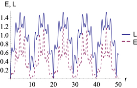
Figure 2. One to one: entanglement dynamics, with  . Blue line:
  red dashed line:
  . Periodicity can be observed here.
Download figure:
Standard image High-resolution imageUnless mentioned, the initial states considered in this paper are the ground state for the uncoupled oscillators, i.e.

which is Gaussian and isn't the true ground state of this Hamiltonian. There are occasions where we don't choose states of this form, but they're still set to be of the form of generalized Gaussian state. Because the Hamiltonian is quadratic and the interactions are bilinear among micro degrees of freedom, for any given Gaussian-type initial state, the final state of the system at later time can be determined analytically. Some details can be found in appendix
It should be emphasized that we only discuss bipartite entanglement between two oscillators, and we adopt the unit  when computing.
Here we introduce two terminologies which will be used later:
- Intra-group entanglement is the entanglement between any two particles of the same group, i.e., entanglement 11 or 22, the meaning of which is explained in figure 1.
- When we choose a particle from each group, the entanglement between these two oscillators is the inter-group entanglement, i.e., entanglement 12.
Next, we introduce the separability criterion and the entanglement measure we will use in this paper.
Peres-Horodecki-Simon criterion
For a state of a continuous system to be separable, Peres-Horodecki-Simon criterion [34–36] is a necessary condition,

where  and
and  is the covariance matrix, the computation of which can be simplified with some tricks as shown in appendix
By Sylvester's criterion2
, a matrix is positive semi-definite if and only if all of its leading principal minors are non-negative. That is, a matrix is positive semi-definite if and only if the determinants of all of its upper-left corner square submatrices and that of the matrix itself are all non-negative. Because  and
and  only differ in the fourth row and fourth column, and because
  is positive semi-definite3
, (3) is equivalent to
is positive semi-definite3
, (3) is equivalent to

Later on we will just call this determinant 
Logarithmic negativity
Logarithmic negativity [38] is defined as4

where  is the partial transpose of ρ and
  It was later proven to be an entanglement monotone, which does not increase under general positive partial transpose preserving (PPT) operations [39]. If the partially transposed state is still a physical state,
  because the density operator is a semi-positive operator whose trace is 1, which implies that a separable state has
  of a Gaussian state can be computed with the covariance matrix [38], and it has been proven that the larger symplectic value doesn't contribute to the entanglement measure [36, 40].
The Peres-Horodecki-Simon criterion implies that for a Gaussian states, it's separable if and only if the covariance matrix of its partial transpose is physically realizable [36, 41], so is the partial transpose itself. Thus, a Gaussian state is separable if and only if both  and
and  are equal to zero.
When we're interested in the degree of entanglement, we will evaluate its  because it's a genuine entanglement measure. As to
  , we keep it as a comparison. Even though being only a separability criterion, not a rigorous entanglement measure,
  somehow can measure the entanglement of a state to some extent. Its dynamical behavior is somewhat like
  as shown in figures displaying entanglement dynamics.
3. Special models
In this section we will discuss three models of which the particle numbers are fixed, and we will show numerical data concerning entanglement, in particular, how the factors of a system with an environment influence the maximal entanglement and disentanglement of a system. Some simple explanations will be provided, which hopefully can help establish a scheme of how entanglement between several parties works.
3.1. One to one
In this model  essentially a pair of coupled oscillators, which shows some basic features that can be helpful in understanding how the entanglement dynamics of coupled oscillators works.
Because of the existence of coupling, the entanglement changes with time instead of staying at where it is initially. Thus, even though the state is separable at the beginning, it becomes entangled immediately.
Due to periodicity, they can become separable again after a finite time. Thus, entanglement sudden death occurs in this model. The wave function is of the form

From (6), we can see that what governs whether these two particles are separable is  . Applying the propagator (32) over an infinitesimal time dt on a wave function whose
  can not vanish, so
  only occurs at discrete values of t. The interaction will make them entangled right after they're separable; in other words, disentanglement can not last for a finite interval in this model.
3.1.1. Entanglement strength
Next we examine how each parameter affects the degree of entanglement, for which an effective way of description is needed. The time evolution of  itself is too complicated to be analyzed directly, so instead we take a numerical approach by finding the maximum value of
  in a given time interval. Plotting the maximum value of
  against a given parameter, this kind of figures can, to some extent, represents how a parameter affects the strength of entanglement. Later on whenever we mention entanglement strength, we are referring to the maximum value of
  for a given system that can be found during its evolution, denoted
  . Please note that entanglement strength as defined here, is by no means a rigorous measure, but of the many aspects of entanglement dynamics it is the one that we focus on in this paper.
From figure 3(a), we find that the larger the coupling strength is, the stronger the maximum entanglement measure is, manifesting the fact that the entanglement is activated by the interaction.
Then, let us see how frequency and mass affect entanglement strength. Figure 3 seems to imply they lower the entanglement strength, but it' is not the whole story. The model has an initial state as (2), which is influenced by frequency and mass as well. It is their roles both in the initial state and the Hamiltonian that causes them to decrease entanglement strength. How they actually influence entanglement strength is superfluous when the degrees of freedom becomes larger and larger as we will see in the following sections.

Figure 3. One to one: maximum values of  as (a) α, (b)
  and (c) m2 change, with
  as default values.
Download figure:
Standard image High-resolution image3.2. One to two
Here  and
and  . It has just one extra oscillator compared to the one-to-one model, yet it makes a huge difference. We neglect the subscript 2 of
  , denoting β.
3.2.1. Environment and entanglement
Now that we have more than two particles, let us discuss the bipartite entanglement between two parties with the presence of a third party, which can be treated as a common environment for the two parties. For such a system, the interaction between the two parties is either direct or indirect, depending on whether the corresponding potential involves only these two parties, which is direct, or also involves the environment, which is indirect. It's apparent that if two parties are separable initially, there should be some form of interactions between them to make them entangled, whether direct or indirect. For example, for parties 1 and 2, their entanglement can be established by party 3 with an interaction term like  even in the absence of terms like
  . Thus, for an open bipartite system, the entanglement of it can be built via the environment, therefore also affected by the environment. Soon we will see how the environment influences the entanglement of a system.
3.2.2. Entanglement strength
The first two diagrams of figure 4 show entanglement strength versus interactions. Here we can see drops and rises, unlike in the one-to-one model. The increase of α increases the entanglement strength of  . The increase of β increases the entanglement strength of
  but decreases
  . This can be understood as follows:

Figure 4. One to two: maximum values of  , blue dots, and
  , red squares, as (a) α, (b) β, (c)
  and (d) m1 vary. Default values:
  . In section 3.1.1, we mentioned that frequency and mass decrease the entanglement strength between a pair of oscillators, and thus
  and m1 drop the direct linkage between 12 and the indirect linkage between 22. The four diagrams all show that indirect linkage has minor influence on entanglement strength in this model.
Download figure:
Standard image High-resolution imageConsider a bipartite system with two parties 1 and 2. Since two separable parties can not be entangled without interaction, unsurprisingly a stronger interaction results in stronger entanglement. There are some parameters that can enhance the entanglement strength, one of which is interaction, while there are some that do the reverse. F us call them entanglement enhancers and reducers.
Now, let us add an environment and treat the whole environment as a party E. Entanglement can be established directly by the interaction between 1 and 2, or indirectly via the environment. When the indirect interaction was turned off, the entanglement strength that would be achievable by the direct interaction alone will be called direct linkage; while if the direct interaction was switched off and the entanglement between 1 and 2 thus would be created via the environment indirectly, the entanglement strength then is called indirect linkage. Entanglement enhancers for 1 and 2 can strengthen the direct linkage, while enhancers for 1 and E, 2 and E, and enhancers for the entanglement within E increase the indirect linkages, similarly for reducers.
Both types of linkages contribute to the entanglement strength between 1 and 2, but their effects don't add up: when one is dominant in a given context, strengthening the other will often decrease the entanglement strength. The graph of  versus a parameter usually can tell us which one holds the rein. For example, if the indirect linkage dominates at a given set of parameters, then the entanglement strength will drop if we enhance the direct linkage a bit. But since sometimes the trend of change is unclear, we can not always be sure of which is dominant. Note that they play unequal roles in determining entanglement strength. Generally, the direct linkage has more weight in this aspect, and it often results in more explicit change in entanglement strength than the indirect one.
3.2.3. Disentanglement
Figure 5 clearly shows that under certain circumstances, entanglement 22 may disappear for a duration, unlike the one-to-one model, where the disentanglement only appears instantly. Due to the periodicity of the system, this disentanglement can not last forever. We will call it finite-life disentanglement from now on, in contrast to finite-time disentanglement [5], or entanglement sudden death [7], which is defined by entanglement disappearing in a finite time rather than asymptotically. Finite life embodies the facts that the disentanglement doesn't last forever and that this phenomenon happens in a finite time. Thus, it is just a special kind of entanglement sudden death. Note that this kind of phenomenon was already discovered [9–11], but to describe it specifically, introducing a simple term seems better than a lengthy description. On the other hand, finite-life disentanglement doesn't happen between 12, on which we provided an argument in [42].
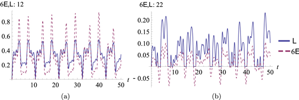
Figure 5. One to two: entanglement dynamics of (a) 12 and (b) 22, with  . Blue line:
  red dashed line:
  . Finite-life disentanglement can appear between 22.
Download figure:
Standard image High-resolution imageIt is interesting to know when finite-life disentanglement can occur between 22. If finite-life disentanglement does happen,  . However, being differentiable to any order,
  should be less than zero during this time interval. Thus, we can find the occurrence of finite-life disentanglement by finding if
  can be less than zero at some time. Here we draw some graphs, as in figure 6, which shows that if the direct linkage becomes weaker or if the indirect linkage becomes stronger, then finite-life disentanglement will be more likely to occur.

Figure 6. One to two: conditions under which finite-life disentanglement between 22 happens. Blue dots are where finite-life disentanglement is found to occur. The pink area is where any of the normal frequencies becomes imaginary, thus excluded. Here we can find that factors that can enhance (weaken) the indirect linkage make finite-life disentanglement more (less) likely to occur, while β, which strengthens the direct linkage, make finite-life disentanglement less probable to happen. (a): at the same α, the weaker β is the denser blue dots are. For fixed β, the blue dots are denser if α is larger. Hence a stronger α, thus a stronger indirect linkage, or a weaker β therefore a weaker direct linkage, makes finite-life disentanglement more probable. (b), (c) and (d): because the increase of m1 and  decreases the indirect linkage, the smaller they are the more likely finite-life disentanglement happens. Default values:
  .
.
Download figure:
Standard image High-resolution image3.3. Boxed cross
The Hamiltonian for this model is

figure 7 gives a schematic graph of the boxedcross model. Its interaction pattern, governed by three parameters, makes this model very interesting. Note that in this model a label is given to each oscillator since they can not be separated into two groups now. Again, we set their states as the initial states of decoupled oscillators, and because they have identical mass and frequency, their initial states are the same.

Figure 7. The boxedcross model. The disks represent oscillators and the two-headed arrows represent coupling between them.
Download figure:
Standard image High-resolution imageFigure 8 shows finite-life disentanglement appearing in this model. figure 9 then exhibits how each interaction parameter changes the entanglement strength, where competition between direct and indirect linkages can be observed.
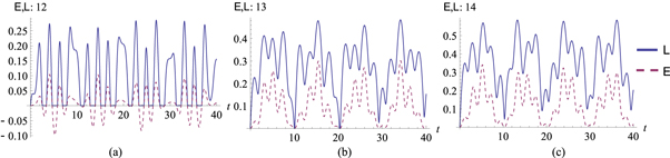
Figure 8. Boxed cross: entanglement dynamics of (a) 12 (b) 13 and (c) 14, with  . Blue line:
  red dashed line:
  . At these parameters finite-life disentanglement is found between 12.
Download figure:
Standard image High-resolution image
Figure 9. Boxed cross: maximum values of  , with
  as default values as (a) α, (b) β and (c) γ change. Blue: 12; red: 13; brown: 14. it is clearly shown that the direct interaction for a pair has strong influence on the entanglement strength. After the initial drop, entanglement strength climbs up significantly.
Download figure:
Standard image High-resolution imageBecause the model is more symmetric than the former one, an empirical relation following which finite-life disentanglement happens can be observed, as shown in figure 10. This figure demonstrates that finite-life disentanglement only happens when the summation of the indirect interactions is stronger than the direct interaction. What we mean by direct and indirect interactions, is that, for example, for the pair 1 and 2, its direct interaction is α, by the Hamiltonian term  , and its indirect ones are β and γ, because 1 and 2 can interact indirectly by the coupling β and γ, as mentioned in section 3.2.1. Thus, for the pair 1 and 2 to have finite-life disentanglement,
  has to be larger than α. Once again, it demonstrates a stronger indirect linkage and a weaker direct linkage make finite-life more likely to happen.

Figure 10. Boxed cross: conditions under which finite-life disentanglement between (a) 12, (b) 13, and (c) 14 happens, with  . Blue dots are where finite-life disentanglement is found to occur. Also, take a look back at figure 6, which looks more complicated, even though the former model per se may seems simpler. This is due to the better symmetry of this model. Finite-life disentanglement happens only if
  and
and  , for these three graphs respectively, for which the oranges lines mark the boundaries. There are some spots where finite-life disentanglement may occur but which aren't found due to limitation of our numerical approach, but there may also be some points in the region at which finite-life disentanglement actually doesn't occur.
Download figure:
Standard image High-resolution imageThe condition that the summation of indirect interactions should be larger than the direct one is only a necessary condition, not a sufficient one. Figure 8 is a good example for illustration. Its three coupling parameters satisfy the triangle inequality, but we only find finite-life disentanglement between 12.
4. General models
In this section we will show the suprema of entanglement of two models whose particle numbers can be adjusted, i.e. how the suprema scale with the system size. Our approach here is analytic and the result is exact without approximation. Even though we make a necessary assumption in order to simplify the algebra, the numerical data confirms the validity of our result. The derivation is given in appendix
4.1. One group
Here we consider the case where there is only one group of identical particles, due to which we drop all the subscripts that specify the groups. We found that, if the particle number N is large enough, it sets an approximate upper bound,  , for entanglement.
The state of our system is always of this form

where a and b are complex. By assuming a and b are real, we can derive6

Note that  is also an upper bound as shown in appendix
  ,
,

where  .
.
What does the above result imply? First, the maximum entanglement achievable by this system is bounded (for  ), which decreases as N increases; second, at larger N, by (10) in a wider range of r will
  be near
  , implying in the whole state vector space the subspace where
  becomes larger. Even though a and b are in general complex, the existence of a least upper bound is consistent with the numerical data to be shown below.
In figure 11, the coupling is set extremely tiny. When the initial state is very close to the ground state of decoupled oscillators, i.e.  and
and  , its maximum entanglement measure is constrained by the weak interaction. There is a region of a and b for the initial state where the maximum entanglement stays at the order of the coupling. This means that, by (10), the ratio
  stays large (assuming they're real) if the coupling is weak. As the initial state moves away from this region, its maximum entanglement starts to climb, up to about
  . Interestingly, even when the ratio
  , the entanglement strength still grows to
  if the a0 is far enough from
  or b0 far enough from 0, namely,
  can become much smaller than N as the state evolves.
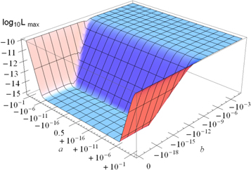
Figure 11. One group: Entanglement strength for different initial states, with  . The initial wave function is
 ![${ \mathcal N }\mathrm{exp}\left[-a{\sum }_{i=1}^{N}{x}_{i}^{2}+2b{\sum }_{i,j\gt i}^{N}{x}_{i}{x}_{j}\right].$](https://content.cld.iop.org/journals/1367-2630/18/7/073001/revision1/njpaa2d35ieqn93.gif) Note that
Note that  and
and  axes scale logarithmically, that the center of the
  axis is 1/2, and that the number shown on this axis should be understood as 1/2 plus the number. For example, if it is
  , its actual value of a is
  . There's a valley around the ground state, which has lower entanglement due to the very tiny coupling β. Except in that region,
  is very close to
  . If β is larger, then the 'valley' will become less apparent, to the point that it can disappear when
  which order depends on other parameters as well. Note that even when the valley disappears,
  will still be very close to
  and this is consistent with (9).
Download figure:
Standard image High-resolution imageNow let us look at figure 12, where we show how the entanglement strength changes as the interaction β changes. Intuitively, when the interaction becomes larger, we expect it to enhance the entanglement strength. In terms of real a and b, this means that a larger β can yield a smaller  Interestingly, from this figure we can observe that the entanglement strength stops growing after it reaches
  , which is exactly the upper bound we found by assuming a and b are real. Note that during the state evolution a and b are rarely real. Therefore, even though a and b are in general complex, the exact upper bound should be very close to or same as the upper bound we proposed, as shown by figure 12(b).

Figure 12. One group: how the interaction β affects the entanglement strength  . (a): I: when β is very tiny, the entanglement strength grows with the increase of
  but it stops growing after the entanglement strength reaches
  . II: because of the initial state, its
  is at about
  even with weak
  I:
I:  and
and  II:
II:  and
and  (b) and (c): The difference is defined as
  , so it must always be positive, whereas the deviation is defined as
  which measures how different it is from the approximation
  . The differences found all being positive, this diagram confirms the supremum we found. Here
  found here are all larger than
  , so we can take the logarithm. The graph shows that
  is indeed larger than
  which is an approximation. I:
  and
and  II:
II:  and
and 
Download figure:
Standard image High-resolution image4.2. Two groups
The state of this system is

for two groups of bosons. In this part we deal only with intra-group entanglement. In previous section we have shown that for the one-group model  . Here we find similar behavior, namely, for the intra-group entanglement
  :
:

as discussed in appendix
Figure 13(a) shows that  stops growing after it reaches
  . Figure 13(b) then shows
  can not surpass
  . We can see the difference is very tiny, but
  just can not exceed the supremum. Finally, figure 13(c), like before, demonstrates
  is just an approximation of
  so
so  can be larger than
  It is still a good approximation for large Ni nonetheless.

Figure 13. Two groups: (a): as  increases,
  climbs till it gets to
  I:
I:  ,
,  ,
,  ,
,  ,
,  II:
II:  III:
III:  (b) and (c) The difference and deviation have the same definitions as in figure 12. Because the differences are all positive as they should be, we take logarithms of them. As to the deviation, it can be both positive or negative because
  . Here
  ,
,  ,
,  ,
, 
Download figure:
Standard image High-resolution image4.3. Two to

In this subsection we will discuss a special case of the two-group model, where group 1, as the system, consists of two oscillators and group 2, as the environment, has a large number of oscillators. We're interested in the entanglement within the system, and that between the system and the environment, i.e. entanglement 11 and 12. The entanglement dynamics of a system consists of two or three oscillators under the influence of a common environment has been studied in work like [43–50]. The phase diagram for general environment, the nonresonant oscillator under weak and strong dissipation, the high-temperature entanglement and the condition for non-equilibrium steady states have been investigated to some extent. Here we would like to add one new perspective — how does the size of the environment affect the entanglement among the system. Unlike previous works, the degrees of freedom of our environment is discrete and finite, so our system never becomes steady, and thus instead of just focusing on the long-time behavior we pick a large number of random time points7 to understand its entanglement property. Calculating how much percentage of the time points when the oscillators in the system are disentangled would tell us how frequent the state of the system becomes separable. We limit the discussion on this model to how α and N2 affect the proportion of time during which the parties under consideration, either 11 or 12, is separable (abbreviated as 'proportion' afterward), shown in figures 14 and 15. Below we will list the trends we observed in the parameter regime we scanned. For entanglement 11
- 1.Increasing both N2 and α makes the system more prone to become separable.
- 2.No matter how large N2 is, α has to be large enough to make the system disentangled.
- 3.If N2 is large enough, at around in this case, further increasing the size of the environment has little influence on the proportion. Likewise, at large N2 and with a large enough α, further enhancing α doesn't make a noticeable difference.
- 4.Because increasing either α or N2 matters little if each is large enough, we conjecture that at given and with a specific initial state, there is a maximum for the proportion in this parameter regime. For the system shown in figure 14 it is about


Figure 14. Two to N2: the three plots show how often 11 is separable, by selecting a large number of random time points and counting the number of points at which the state is separable. For all three plots,  , and the initial state is the ground state when assuming all the oscillators are decoupled. In (a) and (b), we show the proportion of disentanglement, in percentage, as N2 changes. Different curves have different
  as shown beside (b). (a) exhibits the proportion at smaller N2, whereas (b) shows the percentage at larger
  Note that at
  , the proportions are very close or equal to 0. (c) demonstrates the proportion as α varies, with different curves having different
Download figure:
Standard image High-resolution imageAs for entanglement 12
- 1.At small N2, the proportion does not have clear tendency. If N2 is large enough, the proportion increases as N2 gets larger, and it is almost always separable at very large N2.
- 2.At small N2, when changing α we can not really observe an obvious trend. However, at larger N2, we can clearly see a drop of proportion around some value of α. Then the proportion climbs up again as α becomes even larger. With very large N2, the proportion is very high regardless of
- 3.Intuitively, stronger α might have made 12 harder to be separable, which turns out not to be true. It may be because α also makes the indirect linkage stronger. There's a range of value of α that makes a fine balance between direct and indirect linkages. Beyond that value, the indirect linkage dominates.
- 4.As pointed out in section 4, when finite-life disentanglement doesn't happen between 12. However, when N2 is large, it's hard to find when 12 is entangled, which clearly shows the effect of


We should emphasize that due to the nature of randomness, at different runs the results are likely to be different, but not significantly. Besides, there's also no strong reason that a larger N2 or α 'must always' makes 11 or 12 separable more often or not, but the overall tendency can still be found. Please note that in order to keep the eigenfrequencies real and positive, α can not exceed a certain value, which is specific for each system. Therefore it is impossible to take α to infinity without altering other parameters.
5. Discussion
5.1. Entanglement strength
We estimate the entanglement strength by taking the maximum value of the entanglement measure,  , in a finite time. As long as a parameter can change the course of how a state evolves, it can change the entanglement dynamics of a system, but they don't have the same capability in changing the entanglement strength.
To explain how the environment, or the third party, influences entanglement strength, we introduce the idea of direct and indirect linkages in section 3.2.2. In general, a parameter that affects the direct linkage, has more weight in changing entanglement strength than that affecting indirect linkage. Among those influencing the indirect linkage, factors that totally pertaining to the environment are even weaker.
We mentioned that when one linkage is dominant, rising the other often decreases the entanglement strength. We should emphasize that sometimes we can see more than one drops and rises, or no obvious drop on the  versus some parameter graphs. Thus, the direct and indirect linkages work together in a very complicated manner which we don't fully comprehend, or more likely, interpreting it solely by direct and indirect linkages isn't enough.
As discussed in sections 4.1 and 4.2,  may have an inherent upper bound that is determined by the state itself. Hence, no matter how we change the parameters of this system, the entanglement can not go beyond this bound.
5.2. Disentanglement
In our models, we find that the systems can disentangle for a duration, and turn entangled again, which we call finite-life disentanglement. This is interesting for two reasons: (1) this revival of entanglement doesn't come immediately after the disentanglement. After all, the initial state itself is often set to be separable. It's not surprising at all if it merely becomes separable again just in instants; (2) our system is constantly evolving and doesn't stabilize to a certain state, which would make the disentanglement last forever if this particular state is separable. That finite-life disentanglement can even happen in models as simple as the one-to-two model, section 3.2, suggests that such a phenomenon may be more common than we've thought.
If the direct linkage is weaker than the indirect linkage, then finite-life disentanglement becomes more likely to occur. Note that unlike for entanglement strength, for finite-life disentanglement direct and indirect linkages play on a quite even ground, as shown in section 3.3, where we found that the condition for finite-life disentanglement to occur is simply that the sum of indirect interactions should be larger than the direct interaction; on the contrary, even when this condition is satisfied, increasing the indirect interactions and thus the indirect linkage, the entanglement strength often climbs very slowly, and sometimes even drops.
We should emphasize this is an oversimplified interpretation. For instance, it can not explain why finite life disentanglement doesn't happen between 12 for the one-to-two model, section 3.2. The complete mechanism should be more complicated.
One more interesting thing to note: when the indirect linkage is much stronger than the direct one, on one hand the entanglement strength is enhanced, but on the other hand finite-life disentanglement also can become more and more common. Hence raising entanglement strength between two parties may be accompanied with more frequent finite-life disentanglement; they're not mutually exclusive.
5.3. Particle number
5.3.1. Supremum
We found  in section 4.1, and for the two-group model in section 4.2
  . Is this just a coincidence or is there any deeper reason behind? This could be partially answered if we start by observing a spacial class of Gaussian pure states which can be separated into
  , where
  is the state for group i and is also Gaussian. For these particular states,

That is, for these states, the supremum of pairwise entanglement of group i, is equal to the supremum pairwise entanglement of a group of bosons whose state is pure and Gaussian. Hence, for a general two-group Gaussian pure state 

that is, because we've already known the supremum for a special class of states, the supremum of a general state should be equal or larger than it. As it turns out, they are the same, so the possible extra correlation to another group doesn't change the supremum. Does this hold true for an N-group identical oscillator model? This would be a hard problem, but it may be worth further examinations.
These results were derived under the assumption that the state parameters of the wave function are real. However, accompanied with the numerical data, we think even in the more general scenario where those parameters are real, the upper bounds for both cases should be very close to each other. Our results suggests that the entanglement between two parties in a large system will be reduced according to the system size. However, we set a strong constraint on our systems: identicalness. Because the entanglement for a pure bipartite state is unbounded, given a state of this form  , the entanglement between 1 and 2 is unbounded. Thus, that the entanglement is bounded is caused by the identicalness. Besides, the total state is a pure Gaussian state. If it's a mixed Gaussian state, or a more general state, the final results will be possibly different. Still, we think our results are nontrivial, and that similar results, i.e. entanglement scaling with the particle number, possibly in a different way, may be found for other models as well. This can be a route to understanding how entanglement behaves in large systems.
The size of our system is totally under our control. Realistically, the size of a macroscopic quantum system requires some methods to measure and determine [22, 24–26]. Entanglement scaling with the size for other kinds of systems has also been researched, such as area laws [51–53].
It's also worth mentioning an entanglement measure, negativity [38], defined as  , has a similar relation as

5.3.2. Unboundedness when

As shown in appendix  is not bounded from above, and thus it can be any nonnegative number, in sharp contrast to cases where
  Similarly, for two parties that are not identical, we can start from the state (8), knowing this state can have
  as high as we want. Now adjust the state a bit, such that it becomes
 ![$\psi ={ \mathcal N }\mathrm{exp}\left[-{a}_{1}{x}_{1}^{2}-{{ax}}_{2}^{2}+2b{\sum }_{i,j\gt i}^{N}{x}_{i}{x}_{j}\right]$](https://content.cld.iop.org/journals/1367-2630/18/7/073001/revision1/njpaa2d35ieqn181.gif) with a1 very close to a. Because
with a1 very close to a. Because  changes continuously with those state parameters, the resultant state can still have
  as high as we like. Thus, it's not bounded either. Therefore, a bipartite pure Gaussian state has an unbounded
  or more generally, the state of a continuous system in general has an unbounded
5.3.3. Two to N2
In section 4.3 we discussed how an environment with a scalable size influences the entanglement within the system and that between the system and environment. Please note the observations are only applicable to the parameter subspace we've investigated.
We found that a larger N2, thus a larger environment, as well as a larger inter-group interaction α makes 11 disentangled more often. This is because when α and N2 enhance the indirect linkage, the disentanglement becomes more frequent. We also learned that if the environment is big enough, making it bigger doesn't make much difference to how often the system disentangle; similarly, with a large environment if α is strong enough, making it even stronger has little effect on the frequency of disentanglement.
For entanglement 12, the most interesting finding is at large N2 it becomes disentangled very often. If N2 is very large, then it's very hard to find when 12 is entangled. At large N2, we can also see the competition between direct and indirect linkages. Both direct and indirect linkages grow as α is strengthened, but direct linkages loses when α is above a certain strength.
It would be interesting to compare our model with the quantum Brownian motion (QBM) model for two oscillators in the same environment [43, 54]. In QBM models the environment is a collection of independent oscillators with prescribed oscillation frequencies and spectral density. The dynamics of the reduced density matrix is governed by master equations or Langevin equations, where the environment has already been integrated out.
In our model, there is permutation symmetry among each group and the interaction pattern is different from those of QBM. Due to this symmetry, after diagonalizing group 2 there are  degenerate degrees of freedom that are irrelevant to the dynamics of and the entanglement within the system (group 1), as one can see in appendix

Figure 15. Two to N2: the three plots show how often 12 is separable. Like figure 14 
 , and the initial state is the ground state when assuming all the oscillators are decoupled. (a) and (b) show the proportion of disentanglement as N2 changes. (a) and b shows the percentage in different portions of
  (c) demonstrates the proportion as α varies.
Download figure:
Standard image High-resolution image6. Conclusion
Let us summarize what have been found:
- We discussed how a system parameter affects entanglement strength in sections 3.2.2 and 5.1. There we introduced several concepts to interpret the mechanism behind. In whole section 3 were shown several examples.
- Death and revival of entanglement, called finite-life disentanglement by us if the revival doesn't come immediately after the death, can happen in systems as simple as the one-to-two model, section 3.2 and the boxed-cross model section 3.3, implying such a phenomenon should be pretty common. The discussion was in section 5.2.
- The least upper bound of intra-group logarithmic negativity is , i.e. at sufficiently large N, whereas at N = 2 it's unbounded. See sections 4 and 5.3.
- By studying a two-to-N2 model in sections 4.3 and 5.3.3, we demonstrated how an environment with a variable size affects the frequency of disentanglement. One of the important results is that in the parameter regime we investigated, with a large enough environment further increasing the size of the environment will make the entanglement between the system and the environment disappear more often, even to the point that they are almost always separable.
![$\tfrac{1}{2}\mathrm{ln}[1+2/(N-2)]$](https://content.cld.iop.org/journals/1367-2630/18/7/073001/revision1/njpaa2d35ieqn190.gif)

We also noted that it's highly possible that a different state can make the end results distinct from ours. However, it's also possible that other models or systems share some properties in common with those of ours. We hope this article provides some materials for other researchers to examine and compare.
There are many aspects of this model to be explored. For example it would be interesting to investigate more of the two-group model, why at large N2 12 is separable so frequently, and the entanglement between center of mass coordinates. Besides, how to associate the entanglement between large systems and that of their elements shall be studied in more details.
Acknowledgments
This work is partly supported by Ministry of Science and Technology of Taiwan under the grant number MOST 104-2112-M-006-015. The authors acknowledge supports from National Center for Theoretical Sciences (South) and Center for Theoretical Sciences, National Cheng Kung University.
Appendix A.: Evolution of groups of identical oscillators

A.1. Hamiltonian
The Hamiltonian is:

which can be written more elegantly as

where  comprise coordinates of the i-th group, similarly for
  , and
, and  has its elements8
 . Also,

and

Because the matrices  are symmetric (hermitian), they certainly can be diagonalized. By the fact that a rank-N matrix

has eigenvalues a − b and  , the first of them having
  -fold degeneracy. The eigenvector corresponds to the eigenvalue
  is of the form
  which is exactly the center of mass coordinate multiplied by N.
Due to the degeneracy, we can choose any vectors that are mutually orthogonal and orthogonal to  An easy way to finding them all is using the Gram-Schmidt process. For example, we can start from
  , ...,
  Having all vectors normalized will make our work afterward a bit neater. After all this, we have the transformation matrix:
where  . This is an orthogonal matrix, and its inverse matrix thus is its own transpose.
Now let us throw all stuff into the pot. From (17), making the transformation  where
where  is defined as in (21) along with the corresponding momenta
  :
:


where  is
is

We can alternatively write the Hamiltonian as

Note that  . In this Hamiltonian, only virtual oscillators Xi have interactions among themselves, while all other oscillators are isolated. Also, all
  of the same i with
  undergo the same dynamic. We've successfully reduced this Hamiltonian into one with a much simpler interaction pattern.
A.2. Wave function
Under the same Hamiltonian (17) or (25), we want to solve the wave function at time t, whose initial state is9

where

and

Making the same transformation as before, we have10 :

where

We can write it in a more lengthy but enlightening way:
The first and second part evolve on their own, according to the Hamiltonian (25). Therefore, this problem practically becomes solving the wave function of N coupled (virtual) oscillator and that of independent oscillators.
Another interesting thing we can see is that  has to be less than 0 to prevent the wave function from exploding at the boundary. Actually we haven't put any arbitrary constraint on the wave function. If
  , even though it seems to be a 'good' wave function in the original coordinate, indeed the state will fail to satisfy the normalization condition if we really test it by integration.
A.3. State evolution


Appendix B.: Covariance matrices of groups of identical particles
B.1. Expectation value
Because here we have groups of identical particles, instead of really calculating the expectation value of a particular particle, there are many properties to exploit to bypass many procedures. In this system, the primary observables are position and momentum, so we will only consider them. As a reminder,  , and
, and  where
where  is an orthogonal matrix. The particles in the original
  coordinate are identical.
B.1.1. Single position operator
If we want to calculate the expectation value of  since particles of this group are identical, we immediately recognize

B.1.2. Single momentum operator
The momentum operator with respect to Xi is

so we have

B.1.3. Product of operators of the same group
Because we performed an orthogonal transformation,

and

Similarly we have

and

A trickier one:
with which we get

and

B.1.4. Product of operators from different groups
Firstly,

and likely,

B.2. Covariance matrix
If the coordinates  for
for  are still identical after the transformation (21) like our models, then we can simplify our results derived above further. Below are the results. Note that these two matrices are symmetric and that the index j below is always larger than 1, and for this reason we replace
  by
by 
The covariance matrix of two particles from different groups 1 and 2 is
and the covariance matrix of two particles both from the same group is
where for the sack of simplicity we ignore the first index i.
Appendix C.: Entanglement of bosons at gaussian pure states
C.1. One group
The state of this system is of this form

a Gaussian state with permutation symmetry. The logarithmic negativity of Gaussian states is calculated with the methods shown in [38, 40], but in general the final result is too complex to give useful insights. However, if we assume that a and b in (48) are real, then it's possible to reduce it to such a simple form

with basic but lengthy algebras, so we aren't going to show the procedure. The above equation clearly shows that when b = 0 the entanglement measure vanishes, which corresponds to the fact that at b = 0 the state is separable. Hence, we're more interested in circumstances where  , so defining
  we have

There are also constraints for the wave function (48) such that it's square integrable:

taking into account  Now let us discuss the value of d and thus
  by the signs of b.
C.1.1.

d in this case monotonically increases with r, except for the discontinuity at  namely at
  . Under the constraint (51), r never crosses this discontinuity, and thus the suprema of d and
  are given by

because of the monotonicity of the logarithm. Now it's obvious that the maximum value of  decreases as N increases. In addition, at N = 2 both d and
  aren't bounded from above.
At large N, because  for all possible r and therefore we have

Whenever  Hence, the larger N is, the larger the state space where
  is.
is.
C.1.2.

d now monotonically decreases as r increases. Since the discontinuity happens at r = 1, while the constraint (51) requires  , the suprema of d and
  are
are

same as the suprema for  (52). And again at N = 2 there's no upper bound.
As (49) or (50) shows, d adopts different forms according to the sign of b. More interestingly while d for  doesn't depend on
  for
for  does. At first glance there seems to be discontinuity, but as (49) shows d under both circumstances approaches to 0 as b approaching 0, so the entanglement measure changes continuously as b switches the sign.
C.2. Two groups
Now the state is

where X1 and X2 are the normalized center of mass coordinates as defined in appendix A. We want to know the upper bound of  of it. Because the two groups are of the same nature, the upper bound of them should have the same form, and we will just calculate
  Often it's easier to work in the normal coordinate,

where  and
and  are as defined in appendix A and
  and
and  Again assuming
  are all real (so are
  and
and  ), the logarithmic negativity
  of this state can be reduced to
after basic but lengthy algebras. Therefore, d depends on the sign of

C.2.1.

If it's larger than 0, then

As before, there are constraint on these state parameters to make the wave function square integrable. Here, the constraints on b1 and b11 are

If  then
then  because
  and there's no entanglement. Since here we want to find the upper bound of
  we don't have to take this into account. When
  , we only have to consider
  , because otherwise
  .
.
Now assuming  and
and  for the reasons stated above, the last constraint
  leads to

and thus

C.2.2.

If it's smaller than 0, then

To ensure the wave function is square integrable, we need the constraints

which implies

Because d has the same upper bound whether  or
or  , we get

which has the same form as the one-group  except N is replaced by
C.3. The approximation
Let us begin with

 usually is a good approximation for
  for large N. But if we want an approximation that also serves as an upper bound, then
  should be chosen. The reason is

The proof of the above inequality is simple. First,

and thus

meaning that both  and
and  monotonically increase for
  . Because

 and
and  should approaches 0 as
  By their monotonicity, we have

This completes the proof. Therefore,  may be larger than
  but will always be less than
Footnotes
- 2
A more complete description of it can be found in, e.g., [37].
- 3
Thus, all of its principal minors are non-negative.
- 4
In the original paper, it's
instead of . - 5
For the one group model, it is (1) without the second group.
- 6
Note that
isn't , the latter being the maximum for a system while it evolves. - 7
At least 7000 points are picked uniformly over a time interval of more than 7000 units. Because
, a unit of time is the reciprocal of a unit of frequency or energy. - 8
Using a 'normalized' coordinate instead of the center of mass one can prevent many Ni factors from appearing, making it looks tidier.
- 9
The initial state here is any Gaussian pure state, more general than (2).
- 10
Because the transformation matrix is orthogonal, the Jacobian is 1 here.


