


Abstract
Using a stabilizing quadrature-feedback scheme the thermal motion of an on-chip opto-electromechanical resonator is squeezed far beyond the limit of classical parametric squeezing. It is shown that feedback on the Y quadrature by itself can already squeeze the thermal motion of the resonator, but the maximum achievable squeezing level is limited by the imprecision noise. By combining the feedback and parametric pumping a record of 15.1 dB of classical noise squeezing is demonstrated. This not only largely exceeds the 3 dB limit for regular squeezing, but is also deeper than ever can be achieved with feedback cooling. The detector-resonator interaction is analyzed within the semi-classical framework and it is shown that using this feedback-stabilized parametric pumping technique true quantum-squeezed states can be prepared when the resonator starts off close to its ground state, and that the ultimate amount of squeezing depends on the minimum detuning that can be achieved.
Export citation and abstract BibTeX RIS
1. Introduction
Parameteric squeezing is an important and versatile tool to reduce noise in mechanical resonators. Squeezed motion can be generated by different methods such as coupling a resonator to a detector (see e.g. [1]), or by performing backaction-evading or stroboscopic measurements on a single resonator [2, 3]. By coupling different modes in a resonator one can generate correlations between the quadratures of two different modes, creating a so-called two-mode squeezed state [4, 5]. Interestingly, by measuring the motion in the presence of a parametric pump it is also possible to reduce the uncertainty in the position without altering the motion itself [6]. Here we focus on parametric squeezing where the resonance frequency of a single mode of a mechanical resonator is modulated to reduce the thermal vibrations in one quadrature. It is well known that without special techniques this squeezing cannot exceed 3 dB and therefore a feedback scheme is used to greatly enhance the amount of squeezing in our device.
The outline of this paper is as follows: in section 2 the measured parametric squeezing of the thermal motion without stabilizing feedback is discussed as well as the instabilities that limit the noise reduction in that case. Then section 3 studies the dynamics of the system theoretically in the presence of the parametric pump and feedback; the experimental results are presented in section 4. Section 5 shows the ultimate limits on the squeezing with feedback as well as a comparison between quadrature, phase, and regular feedback. Finally, detailed discussions about the operation of the lock-in amplifier, feedback, and measured noise spectra are given in the appendix.
The device [7, 8] that is used in the experiments is shown in figure 1(a). It consists of integrated optical circuits (i.e. waveguides) that form a Mach–Zehnder interferometer. Light is coupled onto and out of the chip using grating couplers (triangular structures). A nanofabricated mechanical resonator in the shape of an H is located near the top arm of the interferometer (see also figure 1(b)). By applying a voltage between its electrodes, the H-resonator is actuated. The displacement u can be measured as a change in the optical transmission through the interferometer. This works as follows: a displacement changes the distance to the nearby waveguide, and thereby the effective index for light travelling through it. This results in a phase shift for the photons travelling in the upper arm of the interferometer, which is detectable in the transmitted optical power. Figure 1(c) shows a measured noise power spectral density (PSD) of the Brownian motion of the resonator. The resonance frequency  of the fundamental in-plane mode is around 773 kHz and the area under the curve is used to calibrate the optomechanical transduction [9]. By applying a static (
 ) and an oscillating voltage between the electrodes, the resonator is excited. The driven response in figure 1(d) shows that the quality factor of this high-stress SiN resonator is about 60 000.
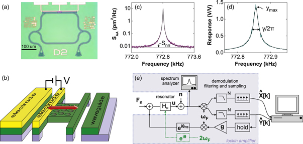
Figure 1. (a) Optical micrograph of a representative device. (b) Schematic of the mechanical part of the device. (c) Power spectral density SAA of the thermal motion of the fundamental in-plane mode of the resonator. The solid line (—–) is a fit to the data and ---- indicates the imprecision noise floor  . (d) Driven response of the resonator with a fit. The width of the resonance is
  and the maximum is
  . (e) Schematic of the feedback system. All the elements in the shaded region are implemented in the lock-in amplifier.
Download figure:
Standard image High-resolution image2. Parametric squeezing
First, the resonator's thermal motion is squeezed by parametrically pumping the resonator with a voltage at twice the resonance frequency without any feedback [10–16]. Due to the electrostatic spring effect in our device this so-called 2f pump modulates the resonance frequency at twice that value. This leads to (classically) squeezed motion where the noise in one quadrature is reduced at the expense of the other.
Two different methods can be employed to analyze the resonator dynamics (figure 1(e)). First of all the detected signal can be demodulated (at frequency  ) using the lock-in amplifier into the X and Y quadratures, sampled, and stored. The resulting timeseries
 ![$\hat{X}[k]$](https://content.cld.iop.org/journals/1367-2630/17/4/043056/revision1/njp512021ieqn7.gif) and
and ![$\hat{Y}[k]$](https://content.cld.iop.org/journals/1367-2630/17/4/043056/revision1/njp512021ieqn8.gif) can then be used to reconstruct the probability density functions (PDFs) [8] that quantify how likely it is to find the resonator at a certain location in phase space. Note that if the sampling is fast enough the sampled data indicated with the index
can then be used to reconstruct the probability density functions (PDFs) [8] that quantify how likely it is to find the resonator at a certain location in phase space. Note that if the sampling is fast enough the sampled data indicated with the index ![$[k]$](https://content.cld.iop.org/journals/1367-2630/17/4/043056/revision1/njp512021ieqn9.gif) accurately represents the underlying timetraces (indicated with
accurately represents the underlying timetraces (indicated with  ) and in the following we will not make this distinction anymore. Secondly, one can also estimate the spectra SXX (f), SYY (f) of the two quadratures which reveal the dynamics of the resonator in the frequency domain. This is done by taking the Fourier transform of
  and
and  and averaging the spectra. This way also the cross-power spectrum
 ![${{S}_{XY}}={{{\rm lim} }_{T\to \infty }}\mathbb{E}\{{{(\mathcal{F}[X(t)])}^{*}}\mathcal{F}[Y(t)]/T\}$](https://content.cld.iop.org/journals/1367-2630/17/4/043056/revision1/njp512021ieqn13.gif) can be obtained, where
can be obtained, where  indicates the expectation value and
  the Fourier transform. The different spectra are related by:

where  is the complex amplitude of the resonator.
Although in principle all these spectra can also be calculated afterwards from the sampled timetraces, this would require excessive amounts of data storage since the spectra require sampling at high rates whereas in order to get enough independent statistics for the probability functions a long measurement record is needed. Therefore these two types of measurements are done separately. Figure 2(a) shows the reconstructed PDFs [8] of the thermal motion for increasing 2f pump amplitude VP. At zero pump power the motion has a circular Gaussian PDF, but by increasing VP the PDF is elongated (amplified) along the Y direction and squeezed along the X direction. To quantify the amount of squeezing, the spectra of the quadrature signals are measured. By integrating the area under the PSDs after subtracting the imprecision background (see figure 1(c)), the variances  and
and  of each quadrature are obtained: these are plotted against VP in figure 2(b). It may seem that by measuring only the spectra, the angular information contained in the trajectories of A(t) is lost as they constitute of projections of A onto the two axes. For example when the squeezing ellipse is oriented
  from X, X and Y are equivalent and both increase with increasing pump strength. In this case, the squeezing effect seems to have been lost in the frequency domain. However, it is still possible to transform the spectra afterward to a different rotated frame (indicated by primes) using:


Here  is the analyzer angle. This allows off-line extraction of the squeezing angle from the measured spectra without requiring access to the underlying timetraces. Figure 2(c) shows the evolution of the two normalized variances when varying α. The two curves show sinusoidal oscillations with a period of
  and a phase difference of
  as expected from equations (2) and (3). By fitting these oscillations, the analyzer angle where the variance in the X direction is minimal,
  , is found. Note that this angle is actually equal to the squeezing angle. By repeating this for each pump amplitude the data in figure 2(d) is obtained. The mean value of
  is close to zero, confirming that the squeezing indeed occurs along the X-axis. This can also be seen in figure 2(a) where the short and long axes of the ellipsoidal PDFs lie along the X and Y axis respectively. The variances obtained from the spectra thus correspond to the minor and major axis of the squeezing ellipse.
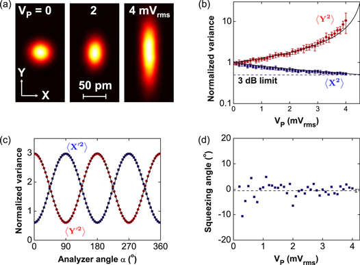
Figure 2. (a) Measured probability density functions of resonator in the presence of a 2f pump with different amplitudes. The left panel shows the unperturbed thermal motion of the resonator. (b) variance of the X and Y quadratures for increasing pump power normalized by  at zero pump power. The dashed line
  indicates the 3 dB limit for parametric squeezing and the solid lines (—–) are a fit of (4) that yields a threshold pump amplitude
  . (c) Dependence of the variances on the analyzer angle α for
  . From the sinusoidal fits (—–) the optimal analyzer angle is found where
  is minimized. (d) Pump-amplitude dependence of
  . The dashed line is the weighted mean value of
  .
.
Download figure:
Standard image High-resolution imageThe theory of parametric squeezing shows that the variances are proportional to  for the squeezed and amplified quadratures respectively. Here γ is the damping rate of the resonator and
  is the strength of the parametric drive [8, 17] (all measurements presented in this work were done at a dc voltage of
  ). The damping in the X direction is thus increased from γ to
  whereas in the Y direction it is reduced to
  . This is the reason why the initially circular PDF becomes ellipsoidal after turning the pump on. The reduction of the noise in the X direction is parametric squeezing and increases with increasing pump amplitude. However, when χ equals γ the damping of the Y quadrature vanishes and at this threshold value
  the system becomes unstable, resulting in large parametric oscillations [18–20]. This happens at a critical amplitude
  , and below this threshold the variances
  and
and  are thus given by:

At the onset of instability the variance of the noise in X(t) is reduced by a factor of 2. This is the so-called 3 dB limit for parametric squeezing. The solid lines in figure 2(b) show the dependences of (4) which fit the data well. The critical amplitude of  is very low compared to other parametric squeezing experiments [10, 18] because of the strong electrostatic interactions in our device geometry.
In this parametric squeezing scheme the pump amplitude thus cannot be increased indefinitely without creating instabilities. One way to circumvent this problem is to do real-time adjustments to the phase of the parametric pump. This naturally leads to the creation of non-Gaussian states as shown in [8]. There, we demonstrated  of squeezing. On the other hand, it is also possible to stabilize the resonator by doing feedback on the amplified quadrature as pioneered by Vinante and Falferi [21]. They squeezed the thermal vibrations of a cantilever whose position is readout using a superconducting quantum interference device. Their squeezing was limited to 11.3 dB but the method itself can lead to much higher degrees of squeezing as we will show here. In this method, the measured Y quadrature of the displacement is fed back to the system by applying a force F(t) to the resonator as shown in figure 1(c). We implement this system in our strongly coupled opto-electromechancial resonator and explore the limits of the squeezing that can be obtained using this scheme. Finally, also in [22] feedback was used, and there −7.4 dB of noise squeezing was reported for externally-driven thermally-broadened states.
3. Oscillator dynamics
The fundamental in-plane mode of the H-resonator studied here can be modelled as a damped harmonic oscillator with mass m, frequency  , and damping rate
  . In the frame rotating at frequency
  the equation of motion for the two quadratures of the resonator can be written in a matrix form. When the resonator is subjected to a parametric modulation of the resonance frequency
  it is given by:

where

is the dynamic matrix and  is the complex force on the resonator in the rotating frame1
. The force F includes the stochastic thermal force noise, the externally applied feedback, and (if present) a driving force.
is the complex force on the resonator in the rotating frame1
. The force F includes the stochastic thermal force noise, the externally applied feedback, and (if present) a driving force.  is the detuning, i.e. the difference between the oscillator frequency and the reference (demodulation) frequency.
In the case of Y-feedback one wants to apply a force on the resonator that is proportional to Y, but the measured value  is not exactly equal to Y. First of all,
  is noisy as one not only detects the resonator displacement u, but also imprecision noise n as shown in the linear system representation of figure 1(e). Moreover, the demodulation of u(t) into X and Y is done using a lock-in amplifier which has a certain frequency response
  around the demodulation frequency due to a finite sampling rate and due to the Nth order low-pass filters; the details can be found in the appendix. Besides the difference between the actual and estimated Y-displacement, the feedback force can have a phase
  with respect to the reference frame, i.e.,
  , yielding
  and
and  , which shows that for feedback on the Y quadrature one needs
  (here ⨂ denotes convolution). Also the feedback gain g (in
  ) is proportional to the experimentally-set value
  (given in
  ) with a proportionality factor
  that is determined from the driven response of the resonator without any feedback or parametric driving (figure 1(d)). After inserting the forces into (5) a new dynamic matrix with the feedback terms
  included is obtained in the frequency domain:

The eigenvalues of M are important to understand the dynamics of the systems and are given by:

An imaginary part of  means oscillatory dynamics around
  whereas the real part of
  determines the damping. The second term makes the real part of the eigenvalues more negative for
  , thereby stabilizing the system. Outside that range the feedback is positive, which destabilizes the system. Note that for real L (corresponding to the case of fast sampling and a large filter bandwidth) the term in the root is always real and hence in this case there are only three possibilities. First of all, when the term in the root is positive there are two different real eigenvalues and the stability of the system depends on the sign of the largest eigenvalue (
 ) as a positive real part implies an instability in the system [23]. Secondly, for a negative value in the root the two eigenvalues have the same real part but opposite imaginary parts. Note that this only occurs for large
  or when the pump and feedback angles are not aligned, i.e.,
  . Finally when the term in the root is zero the two eigenvalues are equal and real.
Without feedback and at zero detuning the two eigenvalues are  and
and  for the X and Y quadratures respectively [10, 21, 24]. These should be compared to the eigenvalue
  of the mechanical resonator itself as illustrated in figure 3(a). When
 ![$\operatorname{Re}[{{\lambda }_{+}}]$](https://content.cld.iop.org/journals/1367-2630/17/4/043056/revision1/njp512021ieqn75.gif) reaches zero at
reaches zero at  , the damping of the other quadrature is twice its original value and the motion in the X-direction is squeezed by 3 dB as mentioned in the discussion of equation (4) above.

Figure 3. (a) evolution of the real part of the eigenvalues with pump amplitude. (b), (d) colorplots of the squeezing in the X quadrature versus pump and feedback strength. The solid line (—–) demarcates the stable and unstable regions (white) for ideal parameters (b) and a small detuning (d). The dotted line in (d) indicates the position of the maximum at a given  . (c) Maximum squeezing in the X quadrature versus Y-feedback gain for different combinations of the detuning, pump angle, and feedback angle. (e) colorplot of D(s) for
  (corresponding to
  ), a sampling rate of
  , and a N = 1 filter with a
  bandwidth, showing three poles. The position of the original (L = 1) eigenvalues is indicated with a ×. (f) Root-locus plot of the poles while decreasing the filter bandwidth. The arrows indicate the movement of the poles when narrowing the filter. The dashed line in (e) and (f) separates the left and right half planes.
Download figure:
Standard image High-resolution imageBy turning the feedback on (figure 3(a)) the system can be stabilized [21] as the real part of eigenvalue that approaches zero for increasing pump amplitude is made more negative. Interestingly, without the parametric pump Y-feedback only changes the real part of the eigenvalues. This is in contrast to regular feedback cooling [9] where both the damping (real part) and frequency (imaginary part) are changed depending on the value of  [25, 26]. Here, when
  and
and  the eigenvalues become
  and
and  [21]. The Y-feedback thus helps to keep the real part of
  negative thus stabilizing the system. This shows that first of all the damping of
  is increased. As illustrated in figure 3(a) this leads to a higher threshold, for example to
  for
for  . At that value the damping of
  is increased to
  (compared to γ without feedback), indicating an additional 1.8 dB of squeezing. The colorplot in figure 3(b) shows the amount of squeezing that is achieved for a given combination of gain and pump amplitude. The largest squeezing occurs at the threshold and is plotted versus
  in figure 3(c). This plot also shows the maximum squeezing in the X quadrature for varying combinations of the feedback angle, pump phase, and the detuning. It is clear that the maximum squeezing at a given g is obtained when all these parameters are zero. In figure 3(d) the case of finite detuning is studied in more detail: first of all the threshold has shifted to larger pump amplitudes and secondly the maximum squeezing in X no longer occurs at the threshold, but at a lower pump amplitude (dashed line). This is due to a rotation of the short axis of the squeezing ellipse away from the preferential X direction. However, even when changing the analyzer direction α (as in figure 2(c)) the maximum achievable squeezing does not recover to the ideal
  case.
case.
So far it was assumed that the feedback happens without delay and with an infinite bandwidth (i.e., L = 1), which is of course not realizable in practice. The influence of the finite sampling rate and filter bandwidth (see appendix) is studied in figures 3(e) and (f). In this case L and hence  depend on ω and the stability of the system is studied by plotting
  against the complex variable s by replacing
  [23]. The poles of the system show up as zeros in this plot. Interestingly the pole corresponding to the eigenvalue at
  has been shifted (blue arrow) to a more negative value due to the finite bandwidth in this particular case. Also, a third pole appeared which did not originate from either of the two original eigenvalues. This pole is caused by the frequency dependence of L. By tracking the position of all poles while decreasing the filter bandwidth the stability of the system can de studied. Figure 3(f) shows that the two leftmost poles move closer and upon touching move away from the real axis. The nonzero imaginary part indicates that the resulting spectrum contains peaks at finite frequency. In this particular parameter set none of the poles crosses to the right half plane indicating that the system is stable. On the other hand increasing the filter order to N = 2 makes the system unstable above a certain gain or below a certain filter bandwidth. Therefore in the experiments we always use a first order filter (see appendix).
The eigenvalues and poles thus play an important role for the stability of the feedback system. However, these do not give a direct answer to the question what the amount of achieved squeezing is. By taking the Fourier transformation of (5) and taking correlations between the different noise terms into account, the noise spectra of the individual quadratures are obtained:


When the force noise only contains thermal force noise (with a constant PSD  ) there is no correlation between FX and FY and hence
  . However, with the feedback on, the force noise also contains the imprecision noise (which enters the through the estimation of the Y quadrature:
 ![$\hat{Y}(t)=L(t)\otimes [Y(t)+{{n}_{Y}}(t)]$](https://content.cld.iop.org/journals/1367-2630/17/4/043056/revision1/njp512021ieqn101.gif) ) that is fed back to the resonator. Combining both contributions yields:
) that is fed back to the resonator. Combining both contributions yields:
where  is the PSD of the imprecision noise. The feedback thus correlates the force noise in the X and Y quadrature as indicated by the nonzero value of the cross-PSD
  . The correlations between the imprecision noise and the force applied to the resonator should also be taken into account when considering the experimentally measured PSDs Sxx and Syy. Doing so yields:

where

The expression for Sxx is simply the sum of the X-displacement PSD and that of the imprecision noise in  (i.e. nX) as the noise fed back to the resonator depends only on the noise in
  (i.e. nY) and is thus uncorrelated with nX. However, such correlations are present in the expression for Syy and this can lead to 'noise squashing', i.e., a reduction of Syy below
  [25–28].
4. Feedback on the Y quadrature
After having derived the theoretical framework in the previous section we now turn our attention to the experiments. In this section we focus on Y-feedback without a parametric pump. Figures 4(a)–(c) show what happens when the feedback angle is varied in the presence of a small feedback gain. Note that for weak feedback both the X and Y spectra remain close to their original Lorentzian shape, but their area and width have been modified by the feedback and have become different for the two quadratures. Figure 4(a) shows the dependence of the variances of the two quadratures as obtained from Lorentzian fits versus the set feedback angle  . For small angles, the fluctuations in the Y quadrature are significantly reduced compared to those in the absence of feedback. When the angle is increased,
  rises and reaches a maximum around
  where the feedback is amplifying the signal. This corresponds to
  and the small difference between
  and
and  is due to delays in the system. When the angle is increased further the variance in the Y direction is again reduced and for
  it is below the variance without feedback. Figure 4(b) indicates that this corresponds to the regions where the damping of the Y quadrature exceeds the intrinsic damping γ. The linewidth extracted from SXX hardly varies with changing feedback phase. Both experimental curves are reproduced by the real part of the eigenvalues given in (8). The variance in the X quadrature only depends weakly on
  . This is because the damping in this direction is unaffected by the feedback (figure 4(b)). Only when
  an increase in
  is visible. This is because the feedback is then mainly in FX resulting in an increased stochastic force on X (see the second term in the expression for
  ). Finally, figure 4(c) shows the difference between the extracted resonance frequency and the reference frequency. As mentioned above, the model does not predict a frequency shift for Y-feedback, but yet a tiny but observable shift is visible (note the change in scale between panels (b) and (c)). This might be due to crosstalk between
  and
and  or due to delays in the feedback loop.
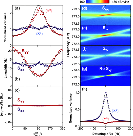
Figure 4. Feedback-angle dependence for  and of the variance (a), linewidth (b), and frequency offset
  (c) extracted from the quadrature noise spectra SXX and SYY. (d)–(g) Colorplots of the noise spectra plotted against the detuning Δ and frequency f for
  . (h) Detuning-dependence of the variances for
  and
and  . The variances in (a) and (h) are normalized by the variances at g = 0. The solid lines (—–) are calculations with values from independent measurements (no free parameters; the difference between
  and
and  is obtained from the phase of the driven response (figure 1(d))).
Download figure:
Standard image High-resolution imageFigures 4(d)–(g) show colorplots of the spectra at a higher feedback gain and varying detuning. The top plot shows SAA and from the asymmetric shape it is clear that the spectrum is no longer Lorentzian. At zero detuning the signal is largest. This is the same for SXX which consists of two peaks that cross: the horizontal one is located at  , i.e., at the resonance frequency
  and the tilted one is located at
  . Now by simultaneously fitting (11) and (12) to the measured Sxx and Syy and integration of (9) and (10) with the resulting fit values for g and
  the variances
  and similarly for
  can be obtained. These are shown in figure 4(h). At zero detuning the X variance is at its original value as it does not experience any feedback. There also the Y variance is at its minimum; at finite detuning the strong reduction in Y is mixed with the unreduced X quadrature and hence the variance in Y increases whereas that of X decreases. At large detuning the two variances approach each other indicating a complete distribution of the thermal energy over the X and Y quadratures. This again shows that the optimal working point is at
  .
.
Figure 5(a) shows the evolution of Sxx at zero detuning when increasing g. No change is observed: both the linewidth and area of the peak stays the same. This is different for Syy (panel (b)). There the sharp peak at g = 0 broadens and its area decreases. At  it is almost indistinguishable from the imprecision background; at larger gains the peak becomes the noise-squashing dip described in section 3. All these features are well described by the fitted theoretical curves, including the rise of the noise at the shoulders of the noise-squashing dip at
  . At this gain, the poles shown in figure 3 have moved away from the real axis, thus creating peaks at a finite offset frequency. The variances are shown in figure 5(c). As expected
  remains at its intrinsic value for all gains, whereas
  first drops steeply with increasing g. It reaches a minimum of 0.058 at
  before rising again. This minimum is well known for regular active feedback cooling [25, 26] and the increase is caused by the imprecision noise that is fed back to the resonator. Therefore the minimum variance depends on the signal-to-background ratio (SBR) between the Brownian motion and the imprecision noise. In the limit
  it is given by
  and occurs at
  [9]. Hence the better the measurement precision is, the lower the variance can become. Our SBR is 30.4 dB (see figure 5(b)) resulting in a minimum normalized Y variance of 0.060 which is close to the observed minimum. At this point it is important to note that by doing feedback on the Y quadrature one also creates a (classically) squeezed state. The feedback increases the damping in the Y quadrature just as the parametric pump did for X in figure 2. This Y-feedback-induced squeezing is illustrated by the PDFs in figure 5(d). Now the minor axis lies along Y and becomes smaller and smaller for increasing gain, following the dependence of
  in panel (c). One important difference when comparing Y-feedback with parametric pumping is that variance in the other quadrature (i.e.
  ) does not increase; the major axis remains constant when the gain is varied. This seems an improvement over the original squeezing scheme that was discussed in section 2; the question why one still wants to use parametric pumping is addressed in the next section.

Figure 5. Noise power spectral density of the X (a) and Y quadratures (b) in the presence of Y-feedback but without parametric pumping. The solid lines (—–) are fits to (11) and (12), respectively. The curves in (a) and (b) are offset from the  case by factors of 10. The inset in (a) shows the same data on a linear scale. (c) The normalized variances plotted against the feedback gain together with the expected dependence for
  (no free parameters). (d) PDFs at different gain settings.
Download figure:
Standard image High-resolution image5. Limits to the squeezing
In the previous section it was shown that even without a pump, Y-feedback by itself can squeeze the resonator motion. The minimum variance and hence the maximum amount of squeezing is determined by the how well the detector can resolve the actual motion above the imprecision noise floor. This situation is in complete contrast to parametric squeezing. There the amount of squeezing does not depend on the detector noise, but only on the stability of the entire system as discussed in section 3: the pump amplitude can be increased until the real part of the eigenvalues in (8) becomes positive. At the optimal conditions  , L = 1, and
  this happens at
  . By increasing the feedback gain further and further, more and more squeezing can be obtained. Perhaps one expects that this would only works up to
  (i.e., up to the minimum in the Y variance versus feedback gain; see for example figure 5(c)) since for higher g the noise in Y increases dramatically. However, equation (7) shows that for
  the two quadratures are uncoupled (the diagonal elements of M are zero). Therefore, even although the noise in the Y quadrature increases for
  , that noise cannot leak to the X quadrature and thus the squeezing in X is not degraded.
Figure 6(a) shows the calculated evolution of the variance in the two quadratures with χ for different values of  . When
  the normalized variance is at 1 and 0.078 for the X and Y variances at
  respectively (note that
  ). When increasing the pump power the variance in the Y quadrature rises steadily, whereas that of the X quadrature keeps decreasing monotonically. They cross around
  , but more importantly
  drops below the variance originally achieved by Y-feedback itself
  for
for  . Then at slightly higher χ it even goes below the minimum achievable feedback cooling limit of 0.060 that requires
  . Right at the threshold (
 ) it reaches a value as low as 0.014, corresponding to 19 dB of squeezing. This is however not the ultimate limit; by further increasing g, even more squeezing can be achieved. This, however, requires the phases and detuning to be exactly zero; plots for finite feedback phase are also shown in figure 6(a). At small pump powers there is no visible difference between the curves, but when approaching the threshold a clear degradation of the squeezing results. By numerically minimizing the variance in the X quadrature versus χ the plots in figure 6(b) are obtained. The minimal variance degrades in a similar fashion when either the detuning, feedback phase, or pump phase nonideal (i.e. not zero). This can be understood as follows: any nonzero value for these parameters couples the squeezed X quadrature to the highly amplified Y quadrature. The noise in the latter will leak to the X quadrature increasing its variance beyond the ideal case. Interestingly, when θ and
  are both nonzero but equal the degradation is less severe; This basically correspond to squeezing in a rotated quadrature
  . Hence, when also the analyzer angle α would be chosen
  the optimal squeezing would be recovered.
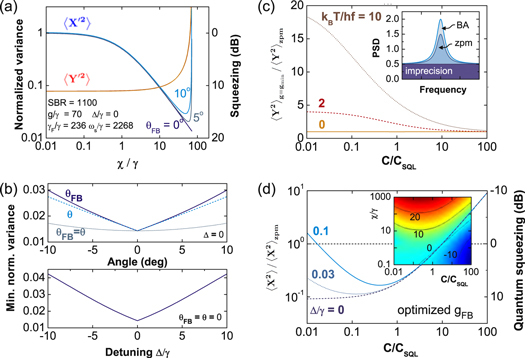
Figure 6. (a) Calculated relative variance for the X and Y quadratures (blue and red hues, respectively) versus the pump strength for  and different values of the feedback angle
  . The three curves for the X quadrature are indistinguishable at this scale. (b) Minimum relative variance of X plotted against three different angles (top) and detuning (bottom). (c) Minimum Y variance relative to the zero-point motion for different coupling strengths between the resonator and the detector for three different temperatures when onlY-feedback is used. The inset shows the noise spectrum components for a quantum-limited detector at the SQL (i.e., for
  ). At the resonance frequency the imprecision background and the backaction (BA) induced motion are both one half of the zero-point motion (zpm). (d) Quantum squeezing of the X variance after optimizing g plotted against the detector coupling at a fixed pump amplitude
  for three different detunings. The inset shows a colorplot of the amount of quantum squeezing in dB when varying both the coupling and pump strength for
  . Both plots are for T = 0.
Download figure:
Standard image High-resolution imageAlthough so far all the experiments were done with a classical resonator, it is interesting to see if this technique is applicable in the quantum regime. For this purpose we analyze a resonator coupled to a quantum-limited (QL) detector in the semi-classical framework [9, 29–31]. By varying the coupling between the detector and the resonator C, a trade off is made between the imprecision at low coupling and detector backaction at large coupling. For a quantum-limited detector (with uncorrelated imprecision and backaction noise) the product of SnnQL and SFFQL is minimal and equals  (for double-sided PSDs) [29]. At the so-called standard quantum limit (SQL), i.e., at
  , the detector backaction on resonance equals the imprecision and their sum in turn equals the intrinsic zero-point motion (zpm) [32] as illustrated by the inset of figure 6(c). This means that the imprecision and force noise PSDs are given by
  and
and  , where the thermal and zero-point fluctuations are included via the Callen and Welton equation [33] and the backaction force is
  . The prefactors are related by
  . Now, for
  the resonator signal is small compared to the imprecision noise of the detector. When Y-feedback is used for a finite temperature resonator the feedback is thus not very effective as shown in figure 6(c). Only by increasing the coupling,
  can be reduced, but for all temperatures it is ultimately limited to the zero-point motion at
  . This means that, as expected from the regular active feedback cooling theory, the feedback alone cannot squeeze the resonator below the zpm. Interestingly, at zero temperature the Y-feedback at optimal gain reduces the variance in the Y quadrature to exactly the zero-point value
  , irrespective of the amount of backaction of the (quantum-limited) detector. Figure 6(d) shows that with the pump on the situation is different. At optimal detuning and low coupling, the fluctuations in the X quadrature are pushed below the zpm and hence true quantum squeezing is achieved. By increasing the coupling the backaction on the resonator increases and this simply degrades the squeezing. At zero detuning the best squeezing is thus obtained for
  . As shown above, classically the squeezing is limited by how well one can determine the resonance frequency, i.e. how small the detuning can be. The same holds for the quantum case. Figure 6(d) shows that for increasing detuning the squeezing is reduced and that for finite detuning there is an optimal coupling. In this case one needs the detector to measure Y(t) in order to cool that quadrature, which requires a finite C. This reduction of
  is beneficial as the finite detuning mixes X and Y. However, after reaching the maximum squeezing at
  the backaction takes over and the squeezing approaches the quickly rising
  curve. The inset shows that increasing the pump power increases the amount of quantum squeezing further and further. It is found that at any detuning the squeezing can be increased by increasing χ. One is thus ultimately limited by either the maximum pump amplitude or the maximum feedback gain that can be applied. Figure 7 shows the experimental data with both the stabilizing feedback and parametric pump enabled. Panel (a) shows the spectra of the X quadrature for a fixed feedback gain and varying pump amplitude, whereas panel (b) shows these for the Y quadrature. Initially Syy shows the characteristic noise squashing dip at zero pump power, but this gradually changes to the reemergence of a peak at higher pump powers. For Sxx the situation is the other way around. At low pump powers the unperturbed thermal motion shows up as a clear peak, but this peak declines and broadens as the pump squeezes the motion in this quadrature further and further. The model described in section 3 can now be used to extract the variances from the spectra. The result is shown in figure 7(c). For different feedback gains
  there are different starting points for
  and also different threshold (i.e., the pump amplitude where
  diverges). However the X-variance follows (4)
  faithfully for all three gain settings up to
  . Beyond that value a saturation is visible and the lowest normalized variance is
  , which corresponds to 15.1 dB of classical squeezing. This value is far beyond the 3 dB limit, and also exceeds the lowest variance that could ever be obtained by active feedback cooling. Moreover, in our strongly interacting electro-optomechanical system the squeezing is larger than previously achieved with similar methods [21, 22] and larger than what we achieved with pump-phase feedback [8]. Although the fits of Sxx fit the data very well, an additional check of the achieved squeezing can be done by numerically integrating the Sxx spectra. Note that (11) shows that everything in Sxx above the imprecision noise floor is resonator motion since there are no correlations between the imprecision noise in X and the feedback force. Numerical integration of Sxx and subtracting the noise floor thus directly gives the variance
  . This gives a maximum squeezing of 15 dB confirming the (more accurate) results obtained from the fitting. Improvements of the squeezing should be possible when increasing the pump power, but this is currently limited by the instrumentation and instabilities in the feedback at very high gains. Finally, the resulting PDFs are shown in figures 7(d)–(f). Clearly the parametric pump and feedback have greatly reduced the occupied phase space. Before (i.e. in panel (a)) the PDF almost entirely consisted of motion whereas in (b) and (c) it contains mainly imprecision noise as indicated by the dashed circle. Yet it is still visible that the PDF is ellipsoidal: the variance in X is smaller than in Y indicating that squeezing by the pump is more efficient than the feedback itself as mentioned above. By improving the detection sensitivity this squeezing becomes more obvious and by measuring a resonator that starts close to its ground state with a quantum-limited detector, the generation of deeply squeezed quantum states should be within reach.

Figure 7. (a), (b) Motion spectra for the X (a) and Y quadrature (b) for different pump amplitudes and a fixed feedback gain. Fits of (11) and (12), respectively, are shown as—-. (c) Extracted variances versus pump power for different feedback gains. Red hues indicate Y whereas blue shades are the X variances. The dashed line  is (4), ⋯⋯ is the 3 dB limit, and ⋯⋯ indicates the lowest variance that is achievable with feedback only. (d) PDF of the thermal motion and (e) PDF of the classical squeezed state for
  and
and  as obtained after optimal filtering. (f) is a zoom of (e) and the circle indicates the size of the imprecision noise.
Download figure:
Standard image High-resolution image6. Conclusion
In summary, we have applied a stabilizing quadrature-feedback scheme to our integrated opto-electromechanical resonator to overcome the 3 dB limit for parametric squeezing. The feedback on the Y quadratures already squeezes the thermal motion, but the minimum achievable variance is bound by the active feedback cooling limit. By combining both the feedback and parametric pumping a record of 15.1 dB of classical squeezing is demonstrated. The amount of squeezing is ultimately limited by the pump power and feedback gain that can be applied to the resonator as well as the minimal detuning. We have shown that the method is also able to produce true quantum-squeezed states when the resonator is coupled to a detector that operates near the quantum limit. Feedback-stabilized parametric squeezing is thus an extremely powerful technique for both the classical and quantum regime of mechanical resonators.
Acknowledgments
M P thanks the Netherlands Organization for Scientific Research (NWO) / M Curie Cofund Action for support via a Rubicon fellowship. HXT acknowledges support from a Packard Fellowship in Science and Engineering and a career award from National Science Foundation. This work was funded by the DARPA/MTO ORCHID program through a grant from AFOSR.
Appendix. Lock-in operation, noise spectra, and frequency response
The demodulation of the lock-in amplifier (Zurich Instruments HF2) can be described as follows: first the incoming signal  is multiplied by
  (see figure 1(e)). Next, this frequency-shifted version of the input is filtered by a cascade of N low-pass filters, each with a time constant
  . This gives a response
  due to the low-pass filtering. Finally the real and imaginary parts of the filtered signal are sampled at a rate fs, resulting in timerecords
 ![$\hat{X}[k]$](https://content.cld.iop.org/journals/1367-2630/17/4/043056/revision1/njp512021ieqn198.gif) and
and ![$\hat{Y}[k]$](https://content.cld.iop.org/journals/1367-2630/17/4/043056/revision1/njp512021ieqn199.gif) where
where ![$\hat{X}[k]=\hat{X}(k/{{f}_{s}})$](https://content.cld.iop.org/journals/1367-2630/17/4/043056/revision1/njp512021ieqn200.gif) . Both the SPA or sample acquisition and the feedback run simultaneously and independently in the lock-in amplifier. They can thus have different sampling rates, filter orders, and filter bandwidths.
. Both the SPA or sample acquisition and the feedback run simultaneously and independently in the lock-in amplifier. They can thus have different sampling rates, filter orders, and filter bandwidths.
To acquire the noise spectra a demodulator with an eight-order (N = 8) filter is used and sampling is done at a rate that is twice the frequency span of the spectrum. The spectra are calculated by taking the digital Fourier transform. The outer quarts are discarded and the resulting spectrum is divided by  (see equations (11) and (12)) to obtain a flat spectrum with aliased components suppressed by at least 35 dB. Finally, note that a signal
  will have a spectral component
  at
at  after demodulation for
  . Its magnitude is thus 1. However, when
  , the Fourier component is only
  . For a randomly distributed ϕ this results in a single point that is 3 dB lower than its neighbors. To avoid artifacts in the spectra this point is omitted.
In the case of feedback a demodulator with a first-order (N = 1) filter is used to keep the dispersion of the phase shift ( ) minimal. This, however, results in significant aliasing of signals outside the frequency range
 ![$\omega /2\pi \in [-{{f}_{s}}/2,+{{f}_{s}}/2]$](https://content.cld.iop.org/journals/1367-2630/17/4/043056/revision1/njp512021ieqn209.gif) . For white imprecision noise with PSD Snn this results in a background of
. For white imprecision noise with PSD Snn this results in a background of  for
for  and
and  . Note that this background is not flat and can be significantly above the noise floor
  that would be obtained when filtering aliased contributions out (e.g. as in the spectrum measurements described above). Moreover, the digital feedback operates in a sample-hold fashion where each measured
 ![$\hat{Y}[k]$](https://content.cld.iop.org/journals/1367-2630/17/4/043056/revision1/njp512021ieqn214.gif) is used for a time
is used for a time  before the next sample
 ![$\hat{Y}[k+1]$](https://content.cld.iop.org/journals/1367-2630/17/4/043056/revision1/njp512021ieqn216.gif) becomes available. This results in an additional delay of
becomes available. This results in an additional delay of  . The total frequency response thus becomes
  .
.
Footnotes
- 1
The factor
 in the definition of the complex force originates from the phase shift between the displacement and a resonant force, whereas the factor 2 ensures that a force with unit amplitude has .


