


Abstract
Seismic source and wave propagation studies contribute to understanding structure, transport, fracture mechanics, mass balance, and other processes within glaciers and surrounding environments. Glaciogenic seismic waves readily couple with the bulk Earth, and can be recorded by seismographs deployed at local to global ranges. Although the fracturing, ablating, melting, and/or highly irregular environment of active glaciers can be highly unstable and hazardous, informative seismic measurements can commonly be made at stable proximal ice or rock sites. Seismology also contributes more broadly to emerging studies of elastic and gravity wave coupling between the atmosphere, oceans, solid Earth, and cryosphere, and recent scientific and technical advances have produced glaciological/seismological collaborations across a broad range of scales and processes. This importantly includes improved insight into the responses of cryospheric systems to changing climate and other environmental conditions. Here, we review relevant fundamental physics and glaciology, and provide a broad review of the current state of glacial seismology and its rapidly evolving future directions.
Export citation and abstract BibTeX RIS
Corresponding Editor Professor Michael Bevis
1. Earth's cryosphere
Earth's water ice cryosphere is a dynamic elastic component of the solid Earth system. The elastic moduli of water ice at seismic frequencies are similar to those of shallow crustal rocks. Thus, internal and boundary dynamic processes, as well as internal structures, of Earth's glaciers and other cryospheric features, are fully amenable to study via seismological methods. The developing field of glacial seismology has thus been able to leverage seismological developments refined across many decades for studying Earth's crust and mantle, as well as a vibrant and diversified seismological community, e.g. Forsyth et al (2009) and strong community geophysical facilities (Aster and Simons 2015). This growth in scientific interest has resulted in a roughly six-fold growth in the cumulative number of scientific papers in the general area of passive glacier seismology between 2000 and mid-2016 (Podolskiy and Walter 2016).
Most generally, we may refer to the seismology of ice or ice-rich Earth materials, structures, and processes as cryoseismology, e.g. Podolskiy and Walter (2016). In this review, we focus on seismic sources and wavefields originating and propagating within glacial ice (figure 1), including those associated with valley and mountain glaciers, ice sheets, ice shelves, and icebergs.
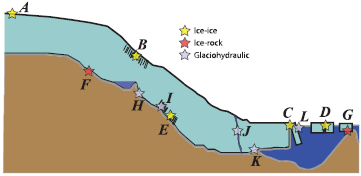
Figure 1. Schematic depiction of a marine-terminating (tidewater) glacial system from icecap source to floating terminus, illustrating seismic source types (stars), identified by source class, and representative citations. (A)–(E): sources associated with ice–ice dynamic processes; (A). Brittle icecap icequakes (Peng et al 2014, Lough et al 2015); (B). Surface crevasse opening or collapse (Neave and Savage 1970, Colgan et al 2016); (C). Calving; (D). Iceberg–iceberg collision, rifting, or fracture (MacAyeal et al 2008); (E). Basal crevasse opening or collapse (Harper et al 2010). (F) and (G): Sources associated with ice-rock stick-slip; (F). Basal stick-slip (Alley 1993, Winberry et al 2009b, Zoet et al 2013); (G). Iceberg grounding (Martin et al 2010a). (H)–(L): Sources associated with ice-water interactions: (H). Subglacial lake drainage and transport (St. Lawrence and Qamar 1979, Harper et al 2005, Winberry et al 2009a); (I). Basal crevasse flow and resonance (Walter et al 2008, Harper et al 2010); (J). Moulin transport and tremor (Röösli et al 2016b); (K). Terminus discharge (Glowacki et al 2016); (L). Iceberg/Calving impact or other dynamic excitation of hdyroacoustic, gravity, and seismic waves via the water column (Bartholomaus et al 2012).
Download figure:
Standard image High-resolution imageAlthough early exploration of the cryosphere and polar regions included geological and geophysical observations, seismological study of the cryosphere, including glacial seismology, developed notably during the 1957–1958 International Geophysical Year, e.g. Sullivan (1961). Extensive seismological study of glacial systems has also greatly advanced during the last two decades, driven by expanding and compelling scientific and societal motivations, and facilitated by dramatically improved new instrumentation technologies and seismic methodologies.
1.1. Glacial systems and the global distribution of glacial ice
The vast majority of ice on Earth today exists in the polar regions (figures 2–6). The volume and geographic distribution of ice has varied tremendously over Earth history on time scales ranging from years to millions of years. This variation principally arises from nonlinear feedback processes occurring between the atmospheric, oceanic, and cryospheric elements of the climate system. Earth's current geographical, geological, and climatological state is amenable to dramatic cryospheric changes, and during the past few million years of Earth history the planet has undergone repeated and extensive glacial- interglacial oscillations.
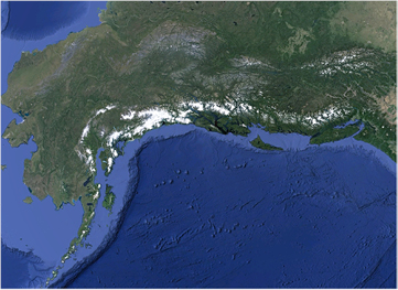
Figure 2. Topographic shaded map showing presently glaciated regions of northwestern North America. Data sources and imagery: U.S. Geological Survey, Scripps Institution of Oceanography, NOAA, U.S. Navy, NGA, GEBCO, PGC/NASA, Landsat, rendered by Google Earth.
Download figure:
Standard image High-resolution image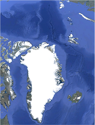
Figure 3. Greenland, northeastern North America, and northernmost Europe. Data sources and imagery: U.S. Geological Survey, Scripps Institution of Oceanography, NOAA, U.S. Navy, NGA, GEBCO, PGC/NASA, Landsat, rendered by Google Earth.
Download figure:
Standard image High-resolution image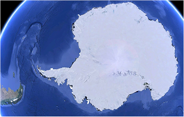
Figure 4. Antarctica and southernmost South America. Data sources and imagery: U.S. Geological Survey, Scripps Institution of Oceanography, NOAA, U.S. Navy, NGA, GEBCO, PGC/NASA, Landsat, rendered by Google Earth.
Download figure:
Standard image High-resolution image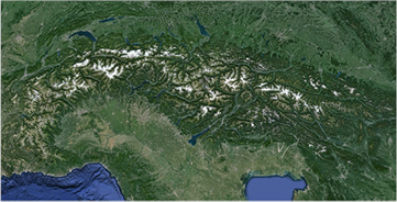
Figure 5. The European Alpine region. Data sources and imagery: U.S. Geological Survey, Scripps Institution of Oceanography, NOAA, U.S. Navy, NGA, GEBCO, PGC/NASA, Landsat, rendered by Google Earth.
Download figure:
Standard image High-resolution image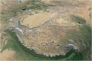
Figure 6. The Himalayan and Tibetan Plateau region. Data Sources and imagery: U.S. Geological Survey, Scripps Institution of Oceanography, NOAA, U.S. Navy, NGA, GEBCO, PGC/NASA, Landsat, rendered by Google Earth: after https://commons.wikimedia.org/wiki/File:Phase_diagram_of_water.svg.
Download figure:
Standard image High-resolution imageThe glacial environment of Earth has exerted profound influence on the evolution of life, and study of glacial conditions and effects across Earth history from recent epochs to deep time is a dynamic field within Earth science, e.g. Macdonald et al (2010). To set the stage for the present glacial cryosphere, we characterize the glaciological history to the Quaternary period (composed of the Pleistocene and Holocene epochs) spanning the most recent approximately 2.5 My of Earth history. During the Pleistocene (2.588–0.0117 My before present), the volume and extent of ice on Earth underwent dramatic and repeated glacial/interglacial cycles, each typically lasting between approximately 40 to 100 kYr. These variations are extensively and widely documented by ice core temperature proxy measurements (e.g. oxygen isotope ratios), glacial landforms, marine sediments, and other paleoclimatological proxies. Aspects of glacial/interglacial cycles have been convincingly linked to insolation variations, and associated feedbacks, arising from periodic astronomically forced orbital and axial inclination changes, including eccentricity, obliquity and precession, referred to as Milankovich Cycles. However, the detailed processes controlling glaciation and glacial cycles, which represent a complex and highly nonlinear interaction between astronomical, atmospheric, oceanic, solid Earth, biological, and other forcing mechanisms, remain an active area of investigation.
The maximal extent of glacial ice during the most recent global glacial advance, referred to as last glacial maximum (LGM; e.g. Clark et al (2009)), occurred approximately 26.5–19.5 Kyr before present. At LGM, extensive ice sheets, with thicknesses of up to several kilometers, covered much of Fennoscandia and North America and, to a lesser extent, southernmost South America. Significantly greater glacial volumes than today also existed in Antarctica and across high mountain regions. Earth presently resides in the interglacial Holocene epoch (0.0117 My present). The International Commission on Stratigraphy (the entity responsible for official geologic time scale designations) is presently considering whether recent and ongoing anthropogenic changes to the planet, including widespread cryospheric melting due to increasing atmospheric and ocean temperatures primarily attributed to increasing atmospheric CO2 and other anthropogenic changes warrant the designation of an Anthropocene epoch or age for the latest Holocene. Despite its lack of formal geological designation, the term 'Anthropocene' is currently in wide colloquial, and sometimes scholarly, use to designate the present geological time.
Seismically relevant glacial features range from millimeters (e.g. crystal scale) to thousands of kilometers (ice sheets). Large (volume greater that 1 km3) glaciers are currently present in North America, Asia, South America, Europe, and Antarctica, as well as higher latitude oceanic island landmasses (notably New Zealand and numerous sub-Antarctic and Arctic islands) (figures 2–6). The ice sheets of Antarctica (≈ ) and Greenland (≈
 ) currently constitute approximately 97% of Earth's glacial area and more than 99% of its volume. Equivalent average global sea level rise for the present land-based Greenland and Antarctic ice masses are approximately 7 and 57 m, respectively (Gregory et al 2004, Fretwell 2013). Non-ice sheet glaciers are concentrated in mountainous regions of the higher-latitude southern and (especially) northern hemispheres. Although non-ice sheet glaciers constitute only a small fraction of the global glacial cryosphere, they have large ecological, climate, and hydrological roles in the natural and human resource landscape (Fountain et al 2012).
The high elevation topographic regions of the ice sheets are slowly flowing domes that transport ice via sheet flow from ice divides, e.g. Fretwell (2013). The largest glacial systems terminate at the oceans. These marine-terminating systems ultimately deliver ice seaward via outlet glaciers (topographically bounded glaciers) and ice stream (ice-flanked streams of faster moving ice) systems (Bentley 1987). In northern Canada, Greenland and Antarctica, some large marine-extending glacial systems terminate in low-topography floating ice shelves. Many other large glaciers, however, terminate more abruptly at the ocean as grounded or floating calving fronts, which may be abutted by an extensive iceberg mélange of calved ice. In both cases, the ocean can exert strong influences on terminus behavior and stability.
2. Physical and seismological properties of glacial ice
2.1. The phase state of glacial ice
Glacial ice under Earth pressure and temperature conditions (0.1–35 MPa (0–4 km ice thickness) and  to
to  C.) resides exclusively in the ice-
 (hexagonal) polymorph (figure 7). The melting under pressure (regelation) of ice near
  C has important consequences for the hydrologic and frictional characteristics of glacial beds, e.g. Weertman (1957) and Clarke (1987) (figure 7). Pure
  ice at
  C and one atmosphere of pressure has a density of 916.79 km
  , which is 91.69% that of liquid water under identical conditions (Lide 2004). The density of terrestrial in situ ice, however, varies widely based on the presence of atmospheric bubbles, rock fragments, and other impurities. The melting-point temperature of ice as a function of pressure can be approximately expressed as a Clausius–Clapeyron relationship

where T0 and P0 are the temperature and pressure of pure water at the triple point ( K and
K and  Pa). The constant γ can range appreciably (e.g.
  K
K  for pure water versus
  K
K  for air-saturated water (Harrison 1975).

Figure 7. Phase diagram of  (log Pressure versus temperature). The approximate glaciological domain on Earth is indicated by the gray box. Background figure compiled from data in www.lsbu.ac.uk/water/phase.html and http://ergodic.ugr.es/termo/lecciones/water1.html after cmglee; https://commons.wikimedia.org/.
Download figure:
Standard image High-resolution imageThe density of freshly fallen snow in cold regions is typically 50–70 kg  . In the absence of surface or sub-surface melt, snow compacts over tens to hundreds of meters, first into compact snow (firn) and eventually into ice with increasing burial depth and pressure, eventually approaching the density of glacial ice with depth (approximately 820–920 kg
  ). Glacial ice is a nearly pure to highly impure polycrystalline solid composed of
  crystals in varying orientations and sizes (typically from sub-mm to many cm).
At time scales exceeding seismic (elastic) periods (i.e. longer than many minutes), glacial ice viscously deforms under deviatoric stress as a strain rate-softening material. The large-strain deformation of glacial ice at these time scales may be grossly characterized by the Glen-Nye law, e.g. Glen (1955),

where η is (temperature- and stress-dependent) power law viscosity

with a rate constant  (dependent on both temperature and ice microstructure and impurities), and
  , C exhibits strong temperature dependence, for example, varying from approximately
  to
to  between 0 and
  C (Cuffey and Paterson 2010).

is the deviatoric stress tensor (the stress tensor, σ minus the mean isotropic stress), and

is the squared maximum shear stress (i.e. the second tensor invariant of d).
While (2) provides a useful formulation for fundamental transport, glacial flow is also influenced by topography, multiple intra- and inter-crystalline creep mechanisms, crystal size distribution, basal or englacial melting, water pathways and inclusions, recrystallization, and temperature profile. Resulting complex strain histories produce spatiotemporally variable, and anisotropic glacial rheology, flow, and fracture structures, e.g. Budd and Jacka (1989). In many cases internal glacial structures can be imaged in substantial detail by land-sited, airborne, or spaceborne ice penetrating radars operating in the MF, HF and VHF frequency bands, e.g. Bogorodsky et al (1985) and Kofman et al (2010).
The broad thermal structure of glaciers may be usefully categorized into warm, cold, and polythermal cases, e.g. Benn and Evans (2014). Warm glaciers occur where summer melt rates are sufficiently high. As a result, the entire ice column is close to the freezing point due to a combination of snow insulation in the winter, and melt, infiltration, refreezing, and latent heat release during summer. Cold glaciers are substantially below the freezing point from surface to base, with very limited or no surface or basal melting, and occur in very cold and dry environments, such as the Dry Valleys of Antarctica. Polythermal glaciers include elements of both warm and cold glacial ice, with their heterogeneous thermal structure reflecting surface and basal conductive and advective heat sources and transport processes (Irvine-Fynn et al 2011), as well as the influence of strain or frictional heating. The Greenland and Antarctic ice caps are broadly polythermal, and basal thermal condition there may be substantially affected by pressure melting, frictional sliding, and geothermal heat flux, while the surface may be uniformly cold, or experience seasonal melt (especially in Greenland).
2.1.1. Seismic waves in ice.
Seismic (elastic) waves in ice, and in solid media generally, are propagating, reversible (or nearly so) elastic strains at frequencies from sub-millihertz to greater than kilohertz. Except in near-source circumstances, seismic strains are usually very small (
 ). In this case, seismic waves are well characterized by linear elasticity theory described by a Hooke's law constitutive relationship of the form

where σ is the (symmetric) stress tensor and  is the corresponding (symmetric, and thus irrotational) strain tensor, both expressed in a common, predefined coordinate system. The stress tensor element
  indicates the xj force component per unit area acting on the xi face of an infinitessimal cube oriented along
  Cartesian coordinate directions. The force vector per area (traction) on a general cube face defined by a unit normal vector
  is thus given by

Note that seismological convention is for extensional strain (and thus extensional stress) defined as positive. Note that this is the opposite to the convention adopted in some other (e.g. engineering) fields.
The seismic strain tensor is defined in terms of displacement,  , Lagrangian spatial derivatives

Following general seismological practice extensional strain is defined as positive.  in (6) is the elasticity (or stiffness) tensor, with elements given by the appropriate elastic constants. Once symmetry and thermodynamic conservation considerations are taken into account, the most general physical (triclinic)
  contains 21 independent constants (e.g. Aki and Richards (2002)). For isotropic media, (6) can be expressed using just two elastic constants as

where λ and μ are the Lamé (elastic) parameters (where μ is the rigidity and λ approaches the bulk modulus as μ approaches zero), and

is the trace of the strain tensor (the dilitation).
The hexagonal symmetry of  of non-randomly oriented ice crystals and/or thin (relative to seismic wavelength) layering due to deposition, flow, and/or compaction, or aligned inclusions of liquid water (Bradford et al 2013) can introduce appreciable bulk elastic rheological anisotropy within glacial ice of up to several percent, e.g. Blankenship and Bentley (1987), Diez et al (2014) and Diez and Eisen (2015) (figure 9). If the elastic properties of a bulk medium are azimuthally isotropic (i.e. anisotropic with a vertical rotational symmetry axis), then the associated elastic anisotropy is referred to as vertical transversely isotropic (VTI). The constitutive relationship for linear elasticity in a VTI solid (6) requires five distinct elastic constants. If the ice contains appreciable crystalline heterogeneity or impurities, such as englacial rock, air, or water, seismic wave propagation for wavelengths substantially longer than size scale of the bulk elastic behavior will be governed by effective (e.g. Voigt-, Reuss-, or Hill-averaged; e.g. Man and Huang (2011)) elastic moduli and density.
The existence of seismic waves in general linear elastic media can be deduced from the equation of motion (Navier's equation) for continuous media expressed in terms of stress, displacement,  , and density, ρ
Specific derivation of seismic wave equations arising from (11) requires the adoption of an appropriate constitutive relationship (6). For isotropic media, using (9), wave equations for elastic wave propagation of P (longitudinal) and S (transverse) (body) waves can be readily derived from (11) (appendix). The nondispersive propagation velocities of P and S waves in this situation are
and

where λ and μ are the Lamé elastic moduli of (9), e.g. Stein and Wysession (1991).
The propagation velocities of P and S waves, in ice are temperature dependent, largely reflecting increasing elastic moduli at lower temperatures. Approximate linear regressions for seismic body wave speeds in isotropic compact glacial ice, compiled from laboratory and in situ measurements of seismic velocities, are (Kohnen 1974)


where T is temperature in °C (figure 8).

Figure 8. Approximate upper and lower compressional and shear seismic wave velocities in isotropic compact glacial ice, from (14) and (15).
Download figure:
Standard image High-resolution imageThese velocities are in the general range of shallow crustal rocks. This ensures appreciable elastic wave coupling between the cryospheric and other parts of the solid Earth. However, in addition to the significantly lesser density, the Poisson's ratio for glacial ice

corresponding to  , is substantially higher than for typical crustal rocks, for which, typically,
  and
and  . Similarly, the bidirectional transmission of elastic wave energy across ice-water interfaces is also significant.
2.2. Snow, firn, and the transformation to glacial ice with depth
The snow-firn-glacial ice transition thickness can exceed 100 m in cold low-accumulation regions (van den Broeke 2008). This transition zone is manifested as a progressive increase in density and elastic stiffness that produces an increasing seismic velocity with depth where vP and vS increase from a few hundred m/s near the surface to glacial velocities (14) and (15), e.g. Albert (1998), Albert and Bentley (1998) and Diez et al (2016). This strong seismic velocity gradient creates a near-surface waveguide for shallowly dipping higher frequency (i.e.  1 Hz) seismic energy (Anthony et al 2015) (figure 9). For glacial systems that are strongly affected by surface melt and ablation, the transition zone will be considerably more complex, or may be absent (in the case of glacial ice exposed by ablation).

Figure 9. (a) Shear wave velocity of the firn to glacial ice transition for the uppermost 150 m of the Ross Ice Shelf at  S and
S and  W, derived from the inversion of Rayleigh and Love surface wave dispersion, using N-S propagating seismic noise recorded by a local seismic array. Green and blue curves indicate Rayleigh wave inversion using data from the vertical and north seismogram components, respectively. Red curve is the velocity inversion from Love waves recorded on the east component. Thin (background) models show 50 representative profiles obtained by fitting surface wave dispersion process using a neighborhood inversion algorithm (Wathelet et al 2004, Wathelet 2008). Corresponding colored thick solid lines show the average model. The individual inversion profiles with the best fit are shown as thick dashed lines keyed by color. (b) Corresponding density profile calculated from the north component (blue line in (a) using the shear wave velocity versus density relationship of Diez et al (2014)). (c) Percentage difference between the S wave velocity profile derived from the north- and vertical-component (green, blue lines) and the north and east component (red and blue line), respectively, showing seismic anisotropy. Reproduced with permission from Diez et al (2016). Copyright © 2016 Oxford University Press.
Download figure:
Standard image High-resolution image2.3. Seismic instrumentation and the seismic noise environment
Seismic sources associated with cryospheric processes exhibit characteristic source durations from thousands of seconds to tens of milliseconds, resulting in seismic radiation across a similar range of periods, e.g. summarized in figure 14 of Podolskiy and Walter (2016). Seismic signals are most commonly detected and studied using seismographic or strainmeter records of surface or subsurface (borehole) ground motion from seismometers installed at fixed (relative to the ice or land surface) geographic locations. Technologies and scientific analysis methods in general solid-Earth and glacial seismology are highly similar and cross-influential, with modifications for glaciological studies usually reflecting specific environmental and/and logistical considerations. As a result, the seismological and glaciological scientific communities and their geophysical instrumentation and facilities have developed increasing levels of collaboration in recent years (Aster and Simons 2015).
Seismic motion is most commonly detected using an electromagnetic inertial seismometer, which may be passive or incorporate active force feedback, damped mass-spring seismometer that produces a vertical- or three-component time series (seismogram) of ground motion. The (typically) analog seismometer output is digitized, time-stamped (usually to a GPS-synchronized clock), and recorded locally and/or telemetered. Modern portable and observatory-based broadband seismographs have useful ground motion responses that can range from many hundreds of Hz to periods of many hundreds of seconds, with a pass band amplitude response that is typically nearly flat to ground velocity within linear bounds. The instrumental noise floor is commonly designed as much as possible to lie below the natural noise floor for seismically 'quiet' sites on Earth (Peterson 1993). Seismic background noise is highly site-specific, and is dictated by a wide range of wind, ocean and other environmental processes, e.g. Dìaz (2016) that produce both quasi-continuous and transient seismic wavefield excitation.
The past two decades have produced a remarkable expansion in seismological data from the cryosphere, collected using both portable (typically seasonal to 1- to 2-year) and long term instrument deployments, such as those of the global seismographic network (GSN) (Butler et al 2004). Important community instrument pools and networks that have seen wide use in the glacial seismology (and broader seismological) research community notably include Incorporated Research Institutions for Seismology (IRIS) Consortium PASSCAL, Polar Instrumentation and UNAVCO geodetic facilities (Aster et al 2005, Nyblade et al 2012) (NSF), global seismographic network (Park et al 2005), GEOSCOPE (Roult et al 2010), GFZ Potsdam GIPP pool (Haberland and Ritter 2016), and SEIS-UK (NERC) facilities. For ground motions at periods beyond the passband of typical seismographic systems (e.g. many hundreds of seconds to thousands of seconds and beyond), larger (e.g. greater than mm-range) surface displacement fields, as well as secular glacial motions may be usefully recorded by geodetic (particularly GPS/GNSS) instruments. Integration of geodetic and seismic observations has been widely utilized to study the full bandwidth of deformation and displacement in seismogenic glaciological processes (Nyblade et al 2012).
The detection and analysis of seismic signals depends on the level of seismic background noise arising from a range of environmental processes. At periods between hundreds of seconds and several seconds, Earth's background seismic noise is dominated the oceanic microseism. The microseism consists of both body and, especially, Rayleigh surface waves, and is globally detectable at all suitably quiet seismic sites (Peterson 1993). Microseism excitation results from energy transfer from ocean gravity waves into seismic waves, principally at or near the coasts, via two distinct mechanisms. The 'primary' microseism is excited by direct ocean swell-coastal interactions, while the more powerful, frequency-doubled 'secondary' microseism is generated by standing-wave components of the ocean gravity wave field), e.g. Longuet-Higgins (1950), Douglas (1977), Ardhuin et al (2011) and Ardhuin et al (2015) that create pressure fluctuations at the ocean floor. Persistent global oceanic excitation of the elastic infrasound field in the atmosphere also occurs, e.g. Ishihara et al (2015). The global microseism noise spectrum has a power spectral density mode dictated by secondary microseism energy between approximately 5 and 10 s period, and a secondary peak or shoulder, representing primary microseism energy, at twice this period. At still shorter periods, seismic noise is commonly dominated by more local wind, water wave, and/or anthropogenic processes (Larose et al 2015). Figure 10 displays a representative probability density function of noise power spectral density for an Antarctic icecap sited station near the Amundsen-Scott Station (U.S.) near South Pole.
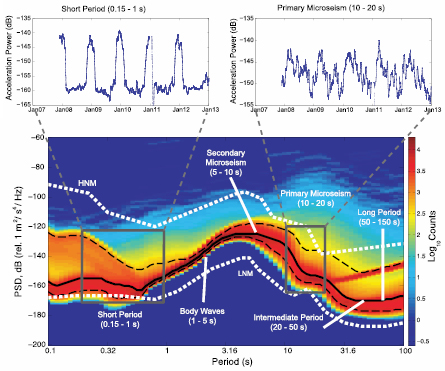
Figure 10. Characteristic seismic signals and noise observed at a broadband seismic station calculated from 1-hour data intervals across five years (December 2007 through December 2012). (a) Probability density function (PDF) of vertical-component seismic acceleration power spectral density (PSD) for global seismographic network (Butler et al 2004) station QSPA. The seismometer is located in a 146 m-deep ice borehole 7.8 km from the Amundsen-Scott South Pole Station (U.S.). White curves (HNM and LNM) show characteristic worldwide high- and low-noise spectral levels, respectively (Peterson 1993). Globally detectable earthquakes are infrequent (visible as low probability, high-PSD features). Six period bands of seismological interest are indicated: Short period (local earthquake/icequake signals commonly observed); Body Waves (dominant P and S body wave global earthquake signals); Primary and secondary microseism bands (ocean wave activity), and Intermediate and long period bands (seismic energy generated by longer-period [infragravity] ocean waves, and seismic surface waves from large global earthquakes). Seasonally-varying annual average power levels in two period bands are shown above (b,c). large annual variability in short period noise reflects anthropogenic austral summer activities at the Amundsen-Scott station. Primary microseism band variations reflect storminess of the Southern Ocean and the annual growth and decay of Antarctic sea ice, which strongly buffers the Antarctic coast from ocean waves during the later austral winter (Aster et al 2008, 2010, Anthony et al 2016). The high probability intermediate to long period PSD swath approaching HNM in this band is from a temporary instrument malfunction. Reproduced with permission from Anthony et al (2015). © 2015 by the Seismological Society of America.
Download figure:
Standard image High-resolution image2.4. Detection and source location of glacial seismicity
Seismic signals from impulsive glaciological processes that exhibit clear P and S phases may be detected and located using standard seismological methods that have been extensively developed by the earthquake seismology community. In this case, determining source location and origin time is a well-posed nonlinear problem that may easily be solved using iterative methods provided the seismic velocity structure can be well estimated and the network of recording stations is sufficiently close to the (3-dimensional) source hypocenter. Given a sufficiently large and well-distributed seismographic network, it is feasible and common to jointly estimate both velocity structure and source locations as an inverse problem, e.g. Zhang and Thurber (2003) and Aster et al (2013) If seismographs geographically encircle the source region, but none are sufficiently close to lying directly above the source, the geographic location (epicenter) may be well determined, but source depth many be poorly constrained. If signal-to-noise ratios are high, event detection is commonly and robustly performed by envelope comparison of short-term and long-term energy averages, e.g. Withers et al (1998). However, where signal-to-noise ratios are low, or where signals are emergent or otherwise do not show clearly interpretable seismic phases due to an emergent or complex source process, or due to complex wave propagation between source and receiver, more advanced methods may be required to detect and locate a seismic source. In this case, incisive amplitude and timing information to assist with source location and other analysis may be extracted from spectrograms, e.g. Martin et al (2010a) and Bartholomaus et al (2012). Coherent arrays of seismographs (in conjunction with individual stations or as networks of arrays), when deployed, facilitate powerful beamforming methodologies that can constrain source location (or azimuth), as well as provide local measurements of apparent wave speed, wave type, and local seismic structure (Diez et al 2016), even for complex sources, e.g. Richardson et al (2012), Köhler et al (2016) and Bromirski et al (2017). For glacial seismic sources that produce a surface manifestation, camera, video, infrasound, and other ancillary instrumentation has obvious utility, e.g. Richardson et al (2010) and Bartholomaus et al (2012).
3. Subglacial stick-slip seismicity
Although internal strain (2) strongly affects general glacial behavior, the most significant processes regulating the translation of glaciers under gravitational driving stress occur at or near the ice-bed interface. Substrate conditions and subglacial water-pressure act in concert to regulate the speed at which glaciers and ice sheets may slide over their beds (Clarke 2005). Many processes relevant to understanding this key aspect of the subglacial environment radiate seismic energy, and/or are associated with strong material contrasts, that allow them to be interrogated remotely with seismology in source and imaging studies.
The majority of the ice-bed interface underlying fast moving glaciers and ice sheets is efficiently lubricated, and the coefficient of friction is sufficiently low, to offer only minimal resistance to forward sliding. In such cases, relatively small regions (<10% of the basal area) of increased friction, know as asperities or 'sticky spots', may oppose substantial percentages of the driving stress (Alley 1993) and thus exert large-scale influences on glacial motion. The presence of localized pinning points can produce basal glacial stick-slip behavior at or around such locations that is analogous to earthquake fault slip in solid-Earth settings, e.g. Brace and Byerlee (1966), generating seismic waves that may be observed and analyzed with remote seismographs.
3.1. Seismic signatures of glacial stick-slip
First proposed by VanWormer and Berg (1970) as a mechanism to explain seismic energy originating from glaciers, it is now clear that seismogenic stick-slip is common within the glacial environment. Basal glacial stick-slip processes have been observed on both large ice sheets and on smaller mountain glaciers across the globe. These diverse environments host asperity patches that span several orders of magnitude in scale, ranging from O(1 m) to O(100 km) (figure 12).
Where recorded with sufficient azimuthal coverage to resolve the pattern of seismic radiation (figure 11), the slip mechanism as well as the size of the slip patch can be estimated using earthquake seismological methods. Analysis of polarity or moment tensor inversion has confirmed that energy radiating for these asperities can be modeled as arising from low-angle thrust faulting (double couple mechanism), consistent with topside motion in the down-glacier direction (Anandakrishnan and Bentley 1993, Walter et al 2009). The seismic moment (A.15) can be estimated from seismograms using the long-period asymptote of the seismic spectrum, while the fall off in spectral amplitude at higher frequency can be used to constrain the slip patch size, allowing the slip, d, to be calculated from (A.15). The spectrum is often fit using

where is fc is the spectral corner frequency and  is the long-period spectral-amplitude at frequencies less than fc. An estimate of the radius, R, (and thus, the slip area, A) of an assumed circular asperity can be estimated using

where vP is the P wave speed for material bounding the fault (Brune 1970).

Figure 11. (A) Estimation of source mechanism and slip patch size from seismic measurements for a group glacial stick-slip events on the Greenland Ice Sheet. The compressive down flow events indicate a thrust type source (Reproduced with permission from Röösli et al 2016a. © 2016. American Geophysical Union. All Rights Reserved.). (B) Estimation of slip patch size from seismic measurements for Antarctic event from P wave displacement spectrum. Solid line is a fit using a theoretical prediction using equation (17). A corner frequency of 100 Hz indicates fault radius of ≈10 m. (Reproduced with permission from Anandakrishnan and Bentley 1993. © International Glaciological Society 1993.)
Download figure:
Standard image High-resolution imageSmaller events (magnitude 0–1), such as those observed beneath both alpine glaciers (Walter et al 2009, Allstadt and Malone 2014, Helmstetter et al 2015b) as well as ice streams (Blankenship et al 1987, Smith 2006, Winberry et al 2013), are most revealingly studied using local (typically up to a few km distant) seismographs due to their small energies. In such cases, dozens to hundreds of distinct bed asperities may be often mapped over relatively small regions (e.g. few square kilometers). Figure 12(a), shows a recent example from the Rutford Ice Stream. Slightly larger slip patches O(100–1000) m, may produce magnitude up to ≈2 events that are readily detectable at regional distances (up to a few hundred km) (Bannister et al 2002, Danesi et al 2007, Zoet et al 2012). Figure 12(b) shows a notable example from the David glacier in Antarctica.

Figure 12. Scales of glacial stick-slip asperities from Antarctica. (A) Top panel shows an example waveform from an ≈1 m asperity, Rutford Ice Stream. Bottom panel shows locations of hundreds of basal icequake events atop high resolution bed topography. Smith et al (2015). (B) ≈1 km, David Glacier. Bottom panel shows Landsat image with event location (Zoet et al 2012). (C) Top panel shows a seismogram from a Whillans Ice Stream stick-slip event associated with an ≈50 km-scale asperity. Bottom panel displays the percentage of total motion that occurs during a slip event. Reprinted from Winberry et al (2011), Copyright (2011), with permission from Elsevier.
Download figure:
Standard image High-resolution imageThe Whillans Ice Stream in Antarctica is home to largest glacial stick-slip events yet noted (Bindschadler et al 2003) (figure 12(c)). During these events, the entire ≈100 km downstream portion of the ice stream moves in approximately twice daily 'slow earthquakes'; 30 min slip events individual seismic moment magnitudes of  . These events were initially detected geodetically via GPS measurements of displacement collected on the glacier surface, but were later found to radiate long-period seismic energy (40–80 s) that can be observed at across Antarctica at distances of up to 1000 km (Wiens et al 2008, Winberry et al 2011). While a single event, each rupture has subsequently been shown to represent the linked breakage of several distinct large asperities (
 5 km radius). This behavior is distinct relative to smaller events, which appear to be isolated asperities that generate several packages of energy observed in far-field seismograms (Pratt et al 2014). Additionally, the ability to jointly observe the Whillans Ice Stream slip events via GPS and seismic instrumentation deployed directly above the slip surface has revealed more detailed evolution of rupture velocity (Winberry et al 2011, Walter et al 2011, 2015b).
3.2. Stick-slip in the subglacial environment
While subglacial stick-slip has been documented across a broad range of spatial scales, a relatively simple model of the process is supported by the observations. In particular, the generation of nearly identical waveforms associated with repeating events indicates repeated slip over isolated subglacial asperities (figure 13) (Smith 2006, Zoet et al 2012, Winberry et al 2013, Allstadt and Malone 2014). We will motivate discussion of subglacial stick-slip mechanics with a relatively simple model that captures its salient features. More detailed and complete summaries of the frictional stick-slip instabilities may be found elsewhere in the seismological literature (Scholz 1998, Marone 1998). We then discuss how the bi-material nature of the subglacial interface (i.e. ice-bedrock or ice-sediment) influences subglacial stick-slip behavior.
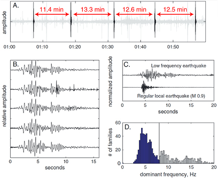
Figure 13. Repeating basal glacial earthquakes from a steep temperate glacier on a dormant volcano (Mount Rainier, Washington, USA). (A). Continuous seismogram showing characteristic near-repeating intervals. (B). Individual (vertical component ground velocity) seismograms from (A). (C). Comparison of glaciogenic events with a tectonic local earthquake, showing unusually low frequency content for an event of this magnitude. (D). Dominant seismogram frequency discriminant developed to separate glacial earthquakes from other seismic events.). Reliable discrimination of glacial, volcanic, and tectonic events on active volcanoes can be a challenge for volcano monitoring (figure 15). Reproduced with permission from Allstadt and Malone (2014). © 2014. American Geophysical Union. All Rights Reserved.
Download figure:
Standard image High-resolution imageAs is frequently done, we will utilize a simple spring slider-block analog to discuss the stick-slip process. The spring is extended at constant rate, resulting in a linearly increasing elastic stress  . If the block is initially at rest, motion will be inhibited until
  exceeds the frictional strength of the block-surface contact, with frictional strength of this interface defined as

where  is effective normal stress, the applied normal stress
  minus pore pressure p, and c is the coefficient of friction, and reflects the sensitivity of basal traction to subglacial hydrologic conditions. This relatively simple relationship between τ and
  can describe basal traction beneath both soft-bedded glaciers (Iverson 2010) and debris laden basal ice sliding over hard beds (Zoet et al 2013).
However, c is not generally constant, but is instead a function of sliding speed, with the simplest case being a static value, cs, while the block is at rest and dynamic value, cd, once the block is moving. If friction increases at the onset of motion (velocity strengthening behavior), the block will slide smoothly. However, if friction drops at the onset of motion (velocity weakening behavior), an instability summarized in figure 14 may arise.

Figure 14. The stick-slip mechanism. The left panel shows a simple spring-slider block system. Extension of the spring, x, applies a force F to the block that is determined by the spring stiffness, K,  (Hooke's Law). Thus, the applied stress
  at the block-surface contact is
  , where A is the contact area between the block and the surface. Motion is resisted by shear stress τ at block-surface contact.
  is the effective normal stress. The right panel shows two stress evolution paths corresponding to unstable (top) and stable (bottom) slip.
  is the distance required for the transition from static friction cs to dynamic friction cd.
Download figure:
Standard image High-resolution imageFirst consider the case where stress levels at Point A in figure 14 initiate slip of a previously motionless block. At the onset of slip,  will begin to decrease as the spring uncompresses due to motion of the block. However, simultaneously, c will decrease as the system transitions to its dynamic value over some finite distance
  . A relatively short time after slip initiation
  . This force imbalance creates an acceleration of the block. The block will continue to accelerate until Point B, after which
  , and the block will begin to decelerate. The block will eventually come to rest at Point C, at which point c will return to its static value. Extension in spring will afterwards accumulate until
  initiates another slip event. This process will produce periodic slip events with a recurrence interval of

This relatively simple model has been implemented (with vary degrees of sophistication) to understand glacial stick-slip at all scales (Bindschadler et al 2003, Winberry et al 2009b, Sergienko et al 2009, Lipovsky and Dunham 2016). It is worth noting that in the glaciological literature, the term 'stick-slip' has additionally been used to describe transitions between periods of minimal and relatively fast subglacial motion that are triggered by diurnal subglacial water-pressure fluctuations (Fischer and Clarke 1997, Boulton et al 2001, Knight 2002, Damsgaard et al 2016). This hydrologic mechanism should not be confused with the rapidly-acting frictional mechanism discussed here that is the driver for seismogenic glacial stick-slip systems.
In subglacial systems, variations in pore pressure are known to drive significant variations in  over time scales ranging from minutes to years. Importantly for stick-slip in glacial systems, the instability of a slip patch with fixed frictional and geometrical properties will be suppressed at effective normal stresses
  below a critical threshold given by

where K is the spring stiffness (Scholz 1998).
Consider the stress evolution when  (figure 14). In this scenario, an initially motionless block begins to move in response to stress conditions represented at Point D. As with the previous case, τ will begin to drop, however, due to the value of
  , the rate of stress reduction occurs at the same rate as the reduction of
  , thus the force balance requires no rapid acceleration between point D and E. When point E is reached, τ remains constant and the block will slide at the rate of spring extension v. However, large perturbations to the background stressing-rate can cause a jump from stable to stick-slip behavior.
In natural systems, the slip behavior is controlled by the elasticity of the materials bounding the slip patch and frictional properties of the interface. We now discuss how the glacial setting influences each of these parameters. From the discussion above, it is clear that the stiffness of system K is fundamental to determining sliding stability. For a slip patch, K dictates the change in stress with slip and is defined as

where μ is the shear modulus of the material bounding the slip interface and L is the length of the slip patch. However, when asperities occur between two strongly contrasting materials μ is not well defined, such as when ice ( Pa) moves over either bedrock (
 Pa) or sediment, (
 Pa) (Iverson et al 1999, Lipovsky and Dunham 2016). When the material contrast is significant, elastic strain will preferentially be accommodated in the more compliant material (figure 15). Thus, for the case of a hard bed asperity, since ice is more compliant than typical bedrock by about an order of magnitude, strain will preferentially be accommodated within the ice at a bedrock contact. During a slip event under such circumstances, the strain in the ice be released due to elastic rebound during the slip. However, for an asperity atop weak sediments, the situation is less clear. The elasticity of sediment is dependent on the particular properties of the material, and its effective normal stress. However, at levels of
  that promote sliding,
  will often be significantly lower than
  and the sediment will accommodate the majority of the inter-event strain (Iverson et al 1999, Lipovsky and Dunham 2016). For both soft and hard bed cases however, net motion only occurs in the ice.

Figure 15. Schematic illustration of asperities on 'hard' and 'soft' beds. When slip is focused on a bi-material interface, strain will preferentially be accommodated in the more compliant material. Thus, for the end-member model of a rigid hard bed asperity, strain is accommodated in ice while the opposite is true for an asperity on a soft bed. As a result, during the slip phase, elastic rebound will primarily occur in the more compliant material. However, irrespective of the materials, net motion only occurs in the overriding ice. Reproduced from Lipovsky and Dunham (2016). CC BY 3.0.
Download figure:
Standard image High-resolution imageIt is worth noting that due to the length of the central Whillans Ice Stream asperity ( 10 km) relative to the ice thickness (≈1 km), this simple model of strain accumulation does not hold. On Whillans Ice Stream, it appears that most inter-event strain is accommodated upstream and downstream of the main sticky-spot (Winberry et al 2014).
This material dependence on strain partitioning has a significant implications for seismic estimation of seismic slip and patch size. To convert the long-period component of the seismogram spectrum into the seismic moment an estimate of the shear modulus is required. Similarly, rupture velocity vr, which controls the duration of the slip event, will be a function of μ, influencing the estimation of slip patch size. Thus, without constraints on material properties of the asperity, authors usually bound estimates for seismic moment, patch size, slip amount with 'hard' and 'soft' bed estimates (Anandakrishnan and Bentley 1993).
Velocity-weakening friction is also a fundamental element for the above stick-slip mechanism. For hard bedded glaciers, insights emerging from limited laboratory studies are showing that the existence of velocity weakening behavior is controlled by ice temperature, basal debris content, and sliding rate (Zoet et al 2013, McCarthy et al 2017). At relatively high temperatures, near the pressure melting point, the production of meltwater reduces steady-state friction by lubricating contacts and promotes velocity strengthening behavior for both clean and debris-laden ice sliding over bedrock. Below the pressure melting point, velocity weakening behavior is favored by increased basal debris contents, while for relatively debris free basal ice, lower temperatures (

 ) appear to promote slip instabilities. For glaciers overriding a soft bed, basal motion may be accommodated by the glacier sliding over the sediment or dominated by sediment deformation near the ice bottom (
 10 m), thus, in many ways similar to gouge in tectonic fault systems. Velocity weakening friction is a common attribute of many granular materials, and significant efforts have been undertaken to constrain the rheological and frictional behavior of subglacial sediments. While these studies reveal that some subglacial sediments display velocity weakening behavior similar to fault gouges, most laboratory results on subglacial sediments tend to display a slight velocity strengthening (or neutral) behavior (Iverson et al 1998, Tulaczyk et al 2000, Rathbun et al 2008). These observations have prompted consideration of velocity-weakening mechanisms associated with pore-pressure reductions in the lee of basal debris as it is dragged through the underlying sediment (Thomason and Iverson 2008) and/or co-seismic pumping and pore pressure change during slip events.
3.3. Insights into subglacial conditions from stick-slip motion
In subglacial environments, resistance to motion is controlled by rheological, stress, and hydrologic conditions. Thus, the stick-slip seismicity offers a window into the temporal and spatial variability of subglacial conditions. Below, we highlight a few of the ways in which stick-slip behavior can be used to illuminate subglacial physical conditions.
3.3.1. Frictional properties of stick-slip.
The generation of stick-slip behavior is dependent on frictional properties ( ). Drivers of this variability may include sediment contrast, basal debris concentration, differing bed types (hard versus soft). As a result, spatial variations in the occurrence of stick-slip behavior may reflect variations in frictional properties.
For example, regions of hard bedded glaciers slightly below their pressure melting point have their sliding stability influenced by basal debris concentration (Zoet et al 2013), a parameter that is likely variable in space. Several studies have suggested that asperities may migrate at rate comparable to ice flow (Zoet et al 2012, Allstadt and Malone 2014, Helmstetter et al 2015b). One potential explanation is that the asperities are generated by regions of high basal debris content that are advected down-glacier. The work of Zoet et al (2012), proposed this as an explanation for a sequence of repeating events effectively turning off after a 9-month period of activity. Thus, at any given location, the frictional conditions that give rise to stick-slip behavior may vary through time.
3.3.2. Hydrologic modulation of seismicity.
 is the dominant control on ice-bed coupling and thus sliding speed for both hard and soft bedded glaciers. As a result, fluctuations in subglacial hydrologic conditions driven from either the input of surface melt-water or internal variability may modulate strength of an asperity. In general, for a given set of frictional properties, regions of high seismicity should be associated with relatively elevated levels of
  . The first compelling evidence of this was provided by Anandakrishnan and Bentley (1993). They observed nearly 200 times more seismic events on the now stagnant Kamb Ice Stream when compared to the neighboring fast moving Whillans Ice Stream. This evidence was used to help corroborate the prevailing hypothesis that the Kamb Ice Stream stagnated ≈150 years ago due to elevated
  . On a more local scale, recent work has confirmed that monitoring the spatial distribution of stick-slip seismicity can be used to infer spatial variability in hydrologic conditions. On the Rutford Ice Stream, regions of high seismicity are associated with areas of 'stiff' till determined independently from active source seismic studies. In contrast, regions identified as high porosity showed minimal seismic emissions, as expected from equation (21) (Smith 2006, Smith et al 2015).
Recent studies have also demonstrated how the temporal behavior of repeating events may illuminate subglacial hydraulic conditions. It is well known that subglacial water systems are comprised of well connected regions as well as poorly connected regions that are less sensitive to transient inputs (Kavanaugh and Clarke 2001, Clarke 2005). These different regions are usually mapped out by drilling multiple boreholes to directly access a broad region of the ice-bed-interface. However, on the margin of the Greenland ice sheet it was recently observed that neighboring asperities (separated by a few hundred meters) displayed contrasting behavior to a diurnal hydrologic forcing. One cluster was modulated by the transient forcing, indicating a connected region of the bed, while a neighboring cluster (a few hundred meters away) displayed no response that is indicative on a hydraulically isolated region of the bed (Röösli et al 2016a). These results suggest that monitoring basal asperities can be used to study the spatial structure of subglacial water systems.
Small magnitude ( ) repeating basal stick-slip events frequently display swarm like behavior, periods of activity followed by quiescence. Allstadt and Malone (2014) observed that the onset of swarms was correlated with relatively modest changes in
  , less than
  0.5% of the glacier load, due to snowfall events. They suggested that this small change in normal stress prompted a reorganization of the hydrologic subglacial system, which in turn the spatial distribution of basal shear stresses and instigated the swarm. However, swarm activity has also been observed in Greenland (Röösli et al 2016a), Antarctica (Smith et al 2015), and other mountain glaciers (Helmstetter et al 2015b) with no clear trigger. However, internally driven oscillations are known to occur in subglacial hydrologic systems (Fricker et al 2007, Schoof et al 2014). Thus, swarm activity may prove useful in tracking spatial and temporal changes in the distribution of subglacial water and stresses (Kavanaugh and Clarke 2001).
3.3.3. Tidal and stressing rate modulation of seismicity.
It is clear from equation (20) that stressing rate variations  will also modulate seismicity patterns. Tidal modulation of the force budget near the grounding lines of marine-terminating glaciers and ice sheets is the best studied driver of variable
  . Tides modulate the glacial force budget through a combination of flexural and hydrologic perturbations that propagate upstream. The speed and magnitude with which a grounding line perturbation propagates upstream is dictated to large degree by subglacial conditions and thus, several studies have demonstrated how along flow observations of tidal influences on seismicity and velocity records can be used to infer subglacial conditions, potentially the appropriate sliding laws (Anandakrishnan and Alley 1997, Gudmundsson 2011, Walker et al 2013). However, in some regions where the surface velocity is tidally modulated, asperities appear to be unperturbed, indicating that the sticky-spots are strong relative to the size of the tidal perturbation (a few kPa) (Aalgeirsdóttir et al 2008, Smith et al 2015).
In the Ross Sea region of Antarctica, a semi-diurnal tide results in peak grounding line flow speeds on the falling tide (Anandakrishnan et al 2003) (figure 16). Analysis of  shows a clear modulation by the tide for both the large Whillans Ice Stream events as well as the smaller David Glacier events. Winberry et al (2009b) and Zoet et al (2012). As expected, higher stressing rates promote a decrease in
  by promoting failure of the asperity earlier in the stick-slip cycle for the David Glacier events. On the Whillans Ice Stream, increasing flow rates near the grounding line on falling tide lead to shorter
  (Bindschadler et al 2003, Winberry et al 2014). It is also observed in both settings that event size scales with inter-event time. This implies that cs is not solely a function on
  , but is a time-dependent feature. This well known behavior is called 'healing' in the rock mechanics literature and is consistent with more complex friction laws (Marone 1998). Several mechanism likely control healing rates in the subglacial environment, but potential processes include increasing contact area between either side of the slip patch with time due to creep of the ice (Zoet et al 2013, McCarthy et al 2017) or pore-pressure diffusion following slip events (Iverson 2010).
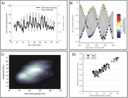
Figure 16. Tidal modulation of stick-slip behavior. (A) Correlation of Ross Sea tides and  for stick-slip events of David Glacier (Reprinted by permission from Macmillan Publishers Ltd: Nature Geoscience Zoet et al (2012), Copyright (2012).). (B) Correlation of Whillans Ice Stream stick-slip events and Ross Sea tides (Reproduced with permission from Winberry et al 2014. © International Glaciological Society 2014). (C)
  versus magnitude for David Glacier events. (D)
  versus magnitude for Whillans Ice Stream events.
Download figure:
Standard image High-resolution image4. Brittle failure seismicity in the interiors of glaciers, ice sheets, and ice shelves
Crevasses are one of the most visible indicators of dynamic behavior in glacial setting, and play an essential role in a range of glacial phenomena (Colgan et al 2016). While satellite imagery provides the spatial resolution required to study fracture processes in glacial systems, it lacks the temporal resolution to resolve short time-scale ( 1 d) processes that characterize fracture evolution. Crevasse formation and expansion in response to glacial stresses generates seismic waves that allow the fracture mechanism to be investigated, providing a complementary tool to other in situ observations (such as GPS). At the smallest scales, firn or exposed ice may produce very small seismic events through consolidation, or in response to boundary or thermal stresses, e.g. Chaput et al (2015).
Across a broad range of glacial settings, small seismic events (magnitudes  to 1) generated by near-surface crevasses are often the most abundant source of seismic activity, allowing development of individual fractures to be monitored, e.g. Neave and Savage (1970) and Rowe et al (2005), while larger events (e.g. magnitudes ≈2) may be observed at relatively large distances (
 800 km) and to exhibit enhanced Rayleigh wave radiation due to their shallow source depths (Lough et al 2015, Mikesell et al 2012). While highly conspicuous on the surface, fractures at depth and in basal context play important roles in the glacial hydrologic system (Fountain et al 2005, Harper et al 2010) as well as in the calving and general stability of ice shelves, e.g. Joughin and MacAyeal (2005) and MacAyeal et al (2003).
Thus, locating seismic activity with high accuracy provides a means of identifying fractures not visible at the surface, e.g. Roux et al (2008). Subsurface fractures may be distinguished from the stick-slip style events discussed above by their predominately isotropic (volumetric) source mechanism. While, the crack opening mechanism is useful for interpreting fracture sources, a few studies have computed the full moment tensor and consistent with theoretical expectations and other observations these studies have shown that shear failure can also be a significant component of the deformation during fracture in glacial settings (Walter et al 2009, Heeszel et al 2014a). Thus, the temporal evolution of seismic activity provides insight into both internal and external drivers of fracture propagation across a range of glacial settings.
On grounded ice, fracture seismicity varies over a range of time-scales in response to both external and internal drivers. In regions associated with surface melt, daily fluctuations in meltwater can modulate seismicity rate by introducing strain-rate variations (Mikesell et al 2012) or through hydrofracturing (Carmichael et al 2012). However, the most significant source of hydrofracturing seismicity is surpaglacial lakes that drain englacially through fractures. During these lake drainage events additional near surface seismicity is driven by glacial deformation as water is redistributed into the sublglacial environment (Roux et al 2010, Carmichael et al 2015). Deformation associated with a passing glacial surge front can drive significant seismicity variations (Raymond and Malone 1986, Stuart et al 2005). At much shorter time-scales it has recently been discovered that transient strain associated with transiting seismic surface waves from large distant earthquakes can dynamically trigger crevasse-attributed seismicity in critically stressed brittle Antarctic glaciers (Peng et al 2014) (figure 17), expanding the field of dynamically triggered remote seismicity, previously recognized in the earthquake system, e.g. Brodsky and van der Elst (2014), into the cryosphere.

Figure 17. Shallow critically-stress crevasse field-attributed icequakes, dynamically triggered in the Newcomer Glacier region of West Antarctica by teleseismic surface waves from a large (Mw 8.8; ≈4691 km-distant) Chilean earthquake (left). At right is shown a vertical-component spectrogram (top) and associated low-pass filtered (colors) seismograms (bottom) showing the arrival of the Love (transversely-polarized) and Rayleigh (vertically-radially polarized) surface waves from the earthquake. The vertically polarized, high-pass filtered seismogram in black shows triggered shallow icequakes induced by the passage of the Rayleigh wave, with timing approximately phase-locked to the maximum Rayleigh wave vertical displacement (and maximum strain dilitation). Reprinted by permission from Macmillan Publishers Ltd: Nature Geoscience Peng et al (2014). Copyright (2014).
Download figure:
Standard image High-resolution image5. Seismicity at marine glacial termini
Iceberg calving from marine and freshwater glacial termini is a complex process that is influenced by glacial strain, gravity waves, tides, currents, surface processes, thermal transport and phase changes associated with both ocean water and glacial ice, sub- and en-glacial hydrology, and by pre- and syn-calving fracturing processes. Calving (and subsequent melting of produced icebergs) is a predominant component of present ice mass loss from Antarctica (Depoorter et al 2013), and also makes up approximately 1/3 of ice mass loss from Greenland (Enderlin et al 2014). Calving is a primary process affecting ice loss and sea level rise that has recently accelerated in many large terminating glacial systems (Thomas et al 2011). This trend has been accompanied by accelerating ice mass loss due to direct melting in Antarctica and Greenland. In Greenland, the predominant process is surface melting and runoff (Enderlin et al 2014). However, in most of Antarctica there is very limited or no surface melting, and accelerated direct melting has recently been driven by warmer ice-shelf water, circulating circumpolar deep water, and by tidal and wind mixing beneath and at the edges of ice shelves (Depoorter et al 2013, Paolo et al 2015).
Calving results from a complex and sensitive interplay of ice dynamics and fracture with associated basal, surface, and terminus thermal and mechanical boundary conditions. This, coupled with its fundamental importance to the behavior and stability of glacial systems, makes the calving regime of historic interest in understanding glacial dynamics. First proposed as seismic source over a half-century ago (Hatherton and Evison 1962), during the past approximately two decades, seismic and other geophysical method have increasingly been applied to studying the calving system.
5.1. Iceberg calving seismicity in Greenland and Antarctica
The Greenland ice sheet, surrounded by coastal mountains, is primarily drained by a small number of very large and fast moving marine-terminating outlet glaciers, some with terminus thicknesses of up to 1 km or more. Enderlin et al (2014) recently estimated that calving from only five Greenland glaciers accounted for approximately 50% (just 15 accounted for 77% and a single glacier, Jakobshavn Isbrae, drains approximately 5 to 8%; Bindshadler (1984)) of icecap mass delivered to the ocean by glacial flow ( Gt) between 2000 and 2014.
The past decade has witnessed dramatic changes in the Greenland ice sheet due to atmospheric and oceanic forcings attributed to climate change. The proportion of ice delivered to the ocean by surface melt and sub- and en-glacial flow has been estimated by Enderlin et al (2014) to now be comparable or greater to the glacial (calving) flux, and to be increasing, (32% to 58% between 2010 and 2014) primarily in response to a climate-change driven increase in surface temperature. Another recent change to the Greenland cryosphere has been the thinning, acceleration and terminus retreat, punctuated by ice mélange and other seasonally variations (Amundson et al 2010) and of large outlet glaciers (for example, over 10 km of recent retreat at Jakobshavn Isbrae; e.g. Joughin et al (2008)).
Greenland and Antarctic outlet glaciers can generate seismic events with source moment magnitudes of up to Mw 5.1 and source durations of 60 s or longer (by comparison, the typical source duration of an Mw 5.0 tectonic earthquake is around 2 s). These events are globally observable as seismic signals with unusually strong Rayleigh waves for their magnitude between 10 and 150 s period (Ekstrom et al 2003, Ekstrom 2006, Ekstrom et al 2006, Tsai and Ekstrom 2007, Tsai et al 2008, Nettles and Ekstrom 2010, Chen et al 2011, Veitch and Nettles 2012). Early source modeling using seismographic data from global distances showed that teleseismic surface waves from these events were inconsistent with tectonic earthquake-like (double couple) source mechanisms, but could be modeled using sub-horizontally directed single-forces applied to Earth's surface in the mass-distance product range (for Greenland) of 0.1 to  kg m (Tsai and Ekstrom 2007). Further global monitoring established their approximate locations at the termini of large tidewater glaciers in both Greenland and Antarctica (but preferentially in Greenland) (e.g. Nettles and Ekstrom (2010)). The spatiotemporal evolution of large Greenland glacial earthquakes show seasonal and secular changes, in particular a northward advancement along the west coast of Greenland over the past two decades, that correlate with atmosphere and ocean warming, suggesting large-scale glaciological response to changing climate (Ekstrom et al 2006, Veitch and Nettles 2012).
Investigations into the source processes of Greenland glacial earthquakes, utilizing seismology, GPS positioning, satellite, and local video observations show that these events arise from glacier, water column, and ocean bed forces applied during the detachment and capsizing of very large ( ) gravitationally unstable newly calved icebergs (Amundson et al 2008, Walter et al 2012, Sergeant et al 2016, Murray et al 2015; (figures 18 and 19). Because larger events are seismically globally observable, their location and magnitudes can be used as valuable proxy measurements to monitor this type of calving. The displacement of large water volumes during these events can additionally generate significant local seiches that apply additional forces to the solid Earth and generate ocean waves that are readily detectable up to 50 km away (Amundson et al 2008). Recent seismic modeling at periods between 10 and 100 s by Sergeant et al (2016) of a particularly well studied megaiceberg calving event (which incorporated two large icebergs) at Jakobshaven showed that at least four important seismogenic mechanisms occurred during the event; collapse initiation, capsizing iceberg-to-terminus contact (distinct for the two associated icebergs), and ice mélange motion (interpreted as sub-horizontal forces generated for 20 min after calving due to collisional or shear forces within the mélange (Amundson et al 2010) and/or along the terminus margin). It appears that the complexity and variability of large glacial calving events results in highly variable seismic excitation, and recent studies incorporating video and other corroborative observations indicate that waveform inversions for moment rate functions of these events may have a limited ability to produce reliable estimates of ice loss (Walter et al 2012, Sergeant et al 2016).
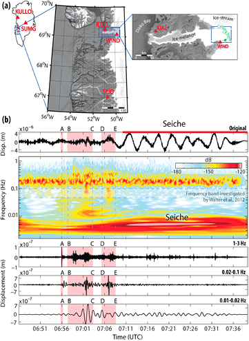
Figure 18. (a) Left: regional seismic stations (red triangles) on the west coast of Greenland used to study megaiceberg calving events at Jakobshavn Isbrae. Right: the glacial fjord and termimus (figure A.1), indicating the source location (Green star). (b) Top: vertical ground displacement at station ILULI and its spectrogram. Bottom: band-pass-filtered seismograms (13, 0.020.1, and 0.010.02 Hz). Attributions of calving event processes, corroborated by video observations, are: (A) ice avalanche at the initiation of calving; ((B) and (C)) initial iceberg capsize; ((D) and (E)) second iceberg calving. Reproduced with permission from Sergeant et al (2016). © 2015. American Geophysical Union. All Rights Reserved.
Download figure:
Standard image High-resolution image
Figure 19. Site and modeling of Helheim Glacier, Greenland megaiceberg calving/capsize glacial earthquake sources during 2013. Map positions are shown in meters in Universal Transverse Mercator zone 24N. The indicated principal force is a reaction force in the up-glacier direction due to the capsizing and rotation of the iceberg. Low pressure behind the rotating iceberg draws water laterally and upwards, which produces a secondary, upward, Earth-normal force. From Murray et al (2015). Reprinted with permission from AAAS.
Download figure:
Standard image High-resolution image5.2. Glacial rumbling and upstream calving-associated slip
Closer inspection from more locally sited seismographs has further revealed that large fast-moving Greenland glaciers can also produce long-duration (10–40 min) 'glacial rumbling' events, such as observed at Jakobshavn to occur approximately once very two days during the summer melt season by Rial et al (2009). These particular events, recorded by a seismographic array at a range near 50 km, were found to commonly culminated in a large-amplitude subevents showing distinct P and S phases that were found to be consistent with fault plane shear (i.e. a double-couple source mechanism) that was geographically associated with a bend in the feeding ice stream. The events had seismic moment magnitudes between approximately 4 and 4.3. However, the sense of slip was not able to be robustly constrained due to a lack of azimuthal source coverage by the available seismic array. Rial et al (2009) interpreted these rumbling events as progressive upstream (5–10 km from terminus) ice–ice or ice-bed stick-slip failure, typically induced by calving events at the terminus.
5.3. Glacial calving seismicity in Alaska and Svalbard
In addition to the major outlets of Antarctica and Greenland, large tidewater glaciers are found in other glaciated regions, including Alaska, Arctic Canada, Patagonia, and Svalbard. The stability of many of these glacial systems appears to be dominated by surface mass balance (Larsen et al 2015), but exceptions exist, including examples of surging mediated by hydrothermodynamic feedback process linked to summer melt noted in Svalbard (Schellenberger et al 2017). Calving dynamics are essential to understanding the full range of tidewater systems on all scales. Particularly well-documented in southeast Alaska, e.g. O'Neel et al (2007), it has long been recognized that calving seismicity may be a useful proxy for calving rate (Qamar 1988, Bartholomaus et al 2012, 2015b, Köhler et al 2015, Köhler et al 2016). Longer term records have been used to understand seasonal fluctuations, surge-type behavior, and dynamic changes during retreat (Walter et al 2010). The seismic and hydroacoustic source mechanisms associated iceberg calving are complex, and include shear and normal forces during detachment and gravitationally driven slip, impact forces of falling ice with the water surface, drag and buoyancy forces associated with ice deceleration, and air/water cavity collapse.
Significant recent progress in understanding seismogenic calving processes has been achieved through simultaneous video/time lapse imagery and seismic observations. Moderate sized calving events involving calved ice volumes of tens to hundreds of thousands of  (i.e. much smaller than the megacalving events of Greenland; figures 18 and 19), and source durations of several to 1000 s), generate local to regionally detectable seismic energy between 0.5 to tens of Hz, that may be strongly peaked in the short period (e.g. 1–3 Hz; O'Neel et al (2007) and Richardson et al (2010)) band (figure 20). A common phenomenon observed to be associated with the generation of this narrowband energy is the generation of air cavity collapse-driven subvertical Worthington jets occurring several seconds after the iceberg impacts the water column (Bartholomaus et al 2012).

Figure 20. Spectrogram of seismic vertical-component velocity of a calving event from Yahtse Glacier in September 2010. Seismogram was recorded 1.8 km from the source on a rock site at the glacier edge. Images at top show the evolution of the calving event, which was visibly identified as initiating at  s on the indicated time scale. The initial, pre-water-column impact, failure of the ice front is associated with weak seismic energy near 5 Hz. The strong spectral peak near 3 Hz is identified with the occurrence of a Worthington (cavity collapse) jet, which becomes visible beginning near
  s. The grounded glacier terminus is approximately 170 m thick and the ice front height extends approximately 60 m above the ocean surface. Reproduced with permission from Bartholomaus et al (2012). © 2012. American Geophysical Union. All Rights Reserved.
Download figure:
Standard image High-resolution imageA long-term goal of glacial seismology is to quantitatively estimate calving rates of marine terminating glaciers at temporal resolution that is not possible with remote-sensing observations. However, at the present state of knowledge, complexity and diversity of calving events (e.g. events with a high degree of subareal fragmentation versus those that are largely submarine) makes the inference of calved ice volumes from purely seismological observables challenging. Calibration for specific glaciers and glacial settings may substantially improve accuracy of these estimates. For example, recent work has shown that relatively simple approaches (generalized linear models) can be used to develop scaling relationships between calving observations (either visual (Bartholomaus et al 2015b) or satellite-derived (Köhler et al 2016)) and seismic attributes, in particular the duration of seismic signal associated with a discrete calving event. Once calibrated, seismic records can then be used to study calving variability over time-windows (daily, seasonal, yearly) during which other observations are not available.
6. Iceberg seismicity
Iceberg collisions and mass wasting processes, e.g. Scambos et al (2008), Glowacki et al (2015) and Scambos et al (2008), are notable contributors to the global oceanic hydroacoustic noise field (Matsumoto et al 2014) and have, more recently, been found to produce significant seismic signals that can be recorded by seismographs at distances of hundreds or even thousands of km (Talandier et al 2006, Martin et al 2010a, 2010b, Pirli et al 2015), where the signals propagate to teleseismic distances as hydroacoustic phases in the oceanic sound channel. Collisions or disintegration of isolated icebergs is also a recognized source of atmospheric infrasound (Richardson et al 2010). The largest marine icebergs originate from Antarctic ice shelves. For example, B15 (calved in March of 2000 from the Ross Ice Shelf), had an extent approximately 120 by 40 km, a thickness between approximately 180–250 m, and a mass of  kg (Dowdeswell and Bamber 2007). The effects of iceberg–iceberg and iceberg grounding contact and seabed scouring are of significant interest in paleoclimatology, biology, marine geology, and a number of other fields (Dowdeswell and Bamber 2007, Martin et al 2010b).
6.1. Iceberg harmonic tremor
Highly harmonic spectral characteristics of some iceberg-associated seismic signals were initially noted from seismic data recorded at Mount Erebus Volcano, Ross Island (MacAyeal et al 2008), in seismic signals recorded on Pacific islands (Talandier et al 2002, 2006) created by coupled hydroacoustic (T) phases (Talandier and Okal 1998, Hanson and Bowman 2006), and in seismograms recorded near the Neumayer Antarctic research station on the Princess Martha Coast of Queen Maud Land (Müller et al 2005). Müller et al (2005) noted the highly harmonic seismic signals (figure 22) associated with the local passage of drifting tabular icebergs, and hypothesized a mechanism involving forced fluid flow and excited resonances. The true mechanism of iceberg harmonic tremor was determined by MacAyeal et al (2008), who exploited a multi-year assemblage of wind and tidally driven, repeatedly colliding large tabular icebergs calved from the Ross Ice Shelf near Ross Island and McMurdo (U.S.) and Scott (New Zealand) Stations (figure 21). This situation facilitated the deployment of iceberg-sited seismographs and GPS positioning instruments to establish both relative iceberg motions and to record associated near-source seismic signals. Iceberg harmonic tremor signals were revealed to arise from repetitive stick-slip events occurring at ice–ice or ice-ground contacts (MacAyeal et al 2015) (figure 22). The harmonic features of these signals arise because impulsive subevents, sufficiently regularly spaced in time, produce harmonic spectra with a fundamental frequency that is equal to the subevent frequency (i.e. a periodic sequence of delta functions has a Fourier spectrum that is a sequence of delta functions in the frequency domain (Bracewell 2000)). The repetitive stick-slip nature of this source process was only revealed when iceberg-sited seismographs were deployed very close (several km or less) to the source zone, because multipathing and attenuation obscure the individual subevents in more distantly recorded seismograms (figure 22).

Figure 21. Seismic station locations and icebergs (MODIS satellite image) near Ross Island, Antarctica on 26 December 2003 Iceberg C16 was immobilized against the northern coast of Ross Island, and the icebergs B15A, B15J, and B15K were adrift at this time. (b) Seismograph sites on C16 (AD) and a land-sites seismograph on Mount Erebus (ABB) (Aster et al 2004) are shown. The collision zone between B15A and C16 was determined to be the source location of prominent iceberg harmonic tremor events. Reproduced with permission from MacAyeal et al (2008). © 2008. American Geophysical Union. All Rights Reserved.
Download figure:
Standard image High-resolution image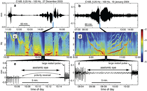
Figure 22. Iceberg harmonic tremor generated by colliding icebergs in the Ross Sea, Antarctica, showing two vertical-component episodes recorded on iceberg C16 seismic station B (figure 1). Respective spectrograms are shown in (c) and (d), where the color bar indicates the  of signal power spectral density in units of dB relative to
  per Hz. Seismic polarity and iceberg motion reversal across seismic gaps, tracking of signal fundamental frequency with the GPS-constrained velocity of B15A, and the polarities of radiated P waves ((e) and (f)) established the source mechanism as repeated strike-slip, stick-slip, subevents occurring at the C16/B15A contact, and driven by reversing relative iceberg motion. Reproduced with permission from MacAyeal et al (2008). © 2008. American Geophysical Union. All Rights Reserved.
Download figure:
Standard image High-resolution image6.2. Iceberg grounding seismicity
Complex seismic and hydroacoustic signals have also been found to be generated during sustained iceberg-seafloor collisions. Martin et al (2010b) analyzed iceberg-sited and remote seismographic recordings of the grounding and breakup of B15A in October 2015 as it collided with an undersea shoal near Cape Adare, Antarctica (figures 23 and 24). This relatively well-studied grounding and breakup event generated powerful harmonic and chaotic signals that were observed as far away as South Pole station (≈ distant; Martin et al (2010b)).

Figure 23. Four successive MODIS images of B15A iceberg breaking up near Cape Adare, northern Victoria Land, Antarctica (250 m resolution). The 250 m depth contour and coast are shown by thin and thick white contours, respectively. The white dot shows the location of a seismograph that was deployed atop the iceberg and recorded its breakup. Reproduced with permission from Martin et al (2010a). © 2010. American Geophysical Union. All Rights Reserved.
Download figure:
Standard image High-resolution image
Figure 24. Spectrogram and corresponding vertical-component seismogram, showing harmonic and non-harmonic signals recorded atop B15 iceberg during its shoaling and breakup, which occurred between October 26 (12:00 UTC) and 28 October (12:00 UTC), 2005. Iceberg tremor events (a)–(c) correspond to the first three panels of figure 23, where events a and b are interpreted as hard grounding events which precipitated iceberg breakup, and event c is interpreted as iceberg harmonic tremor from sideswiping iceberg fragments. Reproduced with permission from Martin et al (2010a). © 2010. American Geophysical Union. All Rights Reserved.
Download figure:
Standard image High-resolution image7. Seismological studies of ice shelves
7.1. Ice shelf seismology
Ice shelves and ice tongues, the floating extensions of ice sheets and glaciers, exert fundamental control on the grounded ice through buttressing. A reduction in buttressing due to collapse or weakening of ice shelves results in the acceleration of inland grounded ice, e.g. Scambos et al (2004), thus accelerating sea level rise. The structural integrity of ice shelves is regulated by the distribution and size of crevasses and rifts (a full depth fracture on an ice shelf). Recent catastrophic ice shelf collapses have been observed to be abetted by the pooling of supra-glacial melt water that promotes hyrofracturing through preexisting fractures and subsequent gravitationally driven disintegration (MacAyeal et al 2003, Scambos et al 2009, Pollard et al 2015), and ice shelves are presently thinning globally in response to changes in ocean temperatures (Paolo et al 2015, Furst et al 2016, Marsh et al 2016, Jeong et al 2016).
Because of importance to glacial stability and sea-level rise, significant efforts are being undertaken to improve understanding of ice shelf structure, dynamics, and stability, including focused seismic studies that illuminate controls on their strain and fracture (rifting and calving) evolution. Ocean swells from distant storms create flexural elastic waves and attendant strains in ice shelves (Bromirski et al 2015) and large icebergs (MacAyeal et al 2006, 2015) that may in some cases promote fracturing (Sergienko 2010). Tsunamis from distant earthquakes have also been observed to spur the calving of large tabular icebergs from ice shelves (Brunt et al 2011). While external environmental factors appear secondary in influencing ice shelf rift propagation (Bassis et al 2007, 2008, Bassis et al 2005), near grounding lines tidal stresses have been shown to exert significant control on fracture rates (Osten-Woldenburg 1990, Barruol et al 2013, Lombardi et al 2016, Hulbe et al 2016) and microseismicity (Podolskiy et al 2016). This is significant, since many ice shelf crevasses originate at grounding lines and are then advected seaward with flow of the ice shelf, where they are increasingly influenced by the ocean.
Recent seismographic deployments atop ice shelves and tabular icebergs (Nicolas et al 1973, Okal and MacAyeal 2006, Bassis et al 2008, MacAyeal et al 2009, Bromirski and Stephen 2012, Zhan et al 2014, Bromirski et al 2015, Diez et al 2016, Bromirski et al 2017), and, in a few cases, on Arctic sea ice (Läderach and Schlindwein 2011) have observed elastic and gravity wave phenomena over periods from thousands of seconds to frequencies of many Hz. Mechanical and other perturbations to ice shelves are of significant importance to assessing the stability of these features. It has recently been discovered that ice shelf displacements also couple into acoustic-gravity atmospheric waves in the 3–10 h period range (Godin and Zabotin 2016).
Harmonic strain from ocean gravity waves may be important to ice shelf stability, e.g. Sergienko (2010), Bromirski and Stephen (2012) Oceanographic mechanical forcings include wind-driven waves and ocean swell, infragravity waves (ocean gravity waves with periods longer than 100 s), tides, ocean gravity wave signals from regional calving events MacAyeal et al (2009), and tsunamis (Brunt et al 2011). Ocean waves (Paolo et al 2015) and tides (Bromirski et al 2015) couple with the sub-ice shelf ocean water column and overlying floating shelf to produce a propagating elastic (compressional, shear, and flexural; e.g. Press et al (1951) and Sergienko (2010)) strain field within the floating glacial ice. Recent large-scale deployment of broadband seismographs across the Ross Ice Shelf has shown that coupled gravity wave/flexural wave strains can penetrate the ice shelf/water cavity system to the ice shelf grounding line (Bromirski et al 2015) (figure 25).

Figure 25. Seismic excitation of the Ross Ice Shelf by ocean waves. (a) Broadband seismograph sites deployed across the ice shelf in the RIS experiment 2014–2016 and from 2004–2006 as part of the pioneering SouthBerg experiment (Cathles et al 2009) (ice-front proximal station NIB). Background color scale shows uncompensated topography with ice removed (Fretwell 2013). (b) RIS broadband array (red star in (a)), showing broadband seismographic stations DR09, DR10, and DR13 for which spectra are calculated. (c) Representative vertical-component acceleration power spectral densities observed at ice front station NIB, DR09, DR10, and DR13, showing the propagation of oceanic-generated flexural wave energy into the ocean cavity and interior of the ice shelf in both the microseism and dwell, and the infragravity wave bands. Reproduced with permission from Bromirski et al (2015). © 2015. American Geophysical Union. All Rights Reserved.
Download figure:
Standard image High-resolution image8. Subglacial and englacial fluvial seismology
Substantial extents of temperate glaciers may be near the melting point, and may thus include liquid inclusions that interact with a melt-containing firn aquifer (Forster et al 2013) and englacial channels affected by melt, crevasse formation, and linked conduits, Fountain and Walder (1998), Irvine-Fynn et al (2011) and Bradford et al (2013). The surface or subsurface transport of water under the influence of gravity or pressurization creates transient forces on the solid Earth that generate seismic waves, e.g. Cole et al (2009), Burtin et al (2010), Schmandt et al (2013) and Burtin et al (2016). Water storage and flow through the surface and subsurface hydrologic pathways of glaciers are central to the transport of heat, to dynamics (e.g. by influencing bed friction; Damsgaard et al (2016)), to erosion, and to mass balance. The flow of fresh water exiting glaciers also strongly impacts the physical and biological state of downstream fluvial, lake, and marine systems. Dynamic glacial processes also create scenarios for meltwater storage and drainage, which may manifest episodically as glacial outburst floods (GLOFs; e.g. Walter et al (2008), Heeszel et al (2014b) and Jacquet et al (2016)) that pose a significant and increasing natural hazard to communities in glaciated regions. Although long recognized for its potential, e.g. St. Lawrence and Qamar (1979), the routine use of seismic methods to explore the glacial hydrologic system has become common only recently, e.g. Bartholomaus et al (2015a). Much of the seismic phenomenology of sub- and englacial flow systems awaits further data collection and study, but recent work point to its potential for monitoring and quantifying the transport of both water and sediment. Terminal flow of subglacial water into the ocean is also a contributor to the hydroacoustic noise field (Glowacki et al 2016). The seismic signature of water movement in glacial systems can be generated by one of two general processes: the resonance of fluid-filled cavities and turbulent water-flow.
In temperate glacial systems, water near the surface is commonly focused into relatively constricted conduits that may take the form of moulins in the englacial environment or basal channels in the subglacial environment mediated by melt and or fracture systems that may be highly seasonally variable (Dalban Canassy et al 2016). This has led many workers to draw parallels between the tremor-like excitation mechanisms of glacial systems and volcanic systems, where the resonance of magma filled conduits is a mechanism for generating band-limited harmonic tremor. If the properties of conduit wall and fluid can be estimated, models of conduit resonance allow the dominant frequency to be related to conduit thickness and width. For example, long duration (6 min) narrow-band (near 3 Hz) tremor recorded in West Antarctica associated with two distinct events of episodic propagation (estimated using array back projection) were linked to the movement of water within sub-ice lake and drainage systems at the MacAyeal Ice Stream (Winberry et al 2009a) (figure 26). Tremor observed on the margin of the Greenland ice sheet has been attributed to the resonance of water-filled moulins, allowing constraints on water depth (Röösli et al 2014). In addition to tremor, the harmonic character of discrete glaciers events (duration of a few seconds) has been related to the transient hydraulic resonant stimulation of fluid-filled fractures at or near the base of glaciers (Métaxian et al 2003, West et al 2011, Heeszel et al 2014b), and within ice shelves (Hammer et al 2015). Some glacial tremor signals exhibit frequency gliding that bears spectral similarity to volcanic and iceberg tremor (Helmstetter et al 2015a). Such frequency-shifting features may result from rapid changes in flow forcing and/or fracture geometry. Ongoing theoretical advances (Lipovsky and Dunham 2015) continue to improve the ability to quantitatively interpret these signals.
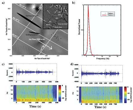
Figure 26. Glaciohydraulic tremor originating beneath the MacAyeal Ice Stream, West Antarctica near its grounding line. The signal is interpreted as a resonating water-ice crack-like conduit with a horizontal dimension on the order of tens of m, draining a small subglacial lake system in episodes lasting approximately 10 min. (a) Location of the MacAyeal Ice Stream (MacIS). Starting and Ending location ellipses show the changing source location of the tremor, estimated using array analysis of seismic energy recorded on the seismographic array indicated by small black triangles. (b) Power spectral density of two tremor episodes, showing narrow-band energy centered near 3 Hz. (C) and (d) show spectrograms (log color scale) showing the sustained, band-limited, and surging nature of the signal with time for two events recorded at a single station. Digitizer counts are proportional to vertical-component seismic velocity. Reproduced with permission from Winberry et al (2009a). © 2009. American Geophysical Union. All Rights Reserved.
Download figure:
Standard image High-resolution imageThe flux of both water and sediments through both englacial and subglacial conduits will vary at both daily and seasonal time-scales. However, continuous high-quality digital seismograms of fluvial systems have only recently been utilized to study seismic signals generated by flow in rivers, e.g. Burtin et al (2010), Schmandt et al (2013) and Burtin et al (2016) and in glacial systems. Bartholomaus et al (2015a) monitored subglacial discharge at the large Mendenhall and Yahtse tidewater glaciers in southeastern Alaska and noted discharge-correlated glaciohydraulic tremor (figure 27). Gimbert et al (2016) studied the relationship between discharge and seismic power at Mendenhall glacier and noted episodic excursions that were successfully modeled using analytical power-law relationships derived for turbulent subglacial conduit flow (figure 28).

Figure 27. Seasonal glaciohydraulic tremor interpreted as being due to near-terminus subglacial flow at Yahtse Glacier, Alaska between July 2009 and October 2011 (a) selected station locations and color-coded relative tremor amplitude. (b) Vertical-component velocity seismic spectrogram for station LUPN (c) Vertical-component seismic velocity amplitude of tremor for the three indicated stations shown in (a). (d) Estimated total, rain, and glacial melt water input to the system for the same time period. Reproduced with permission from Bartholomaus et al (2015a). © 2015. American Geophysical Union. All Rights Reserved.
Download figure:
Standard image High-resolution image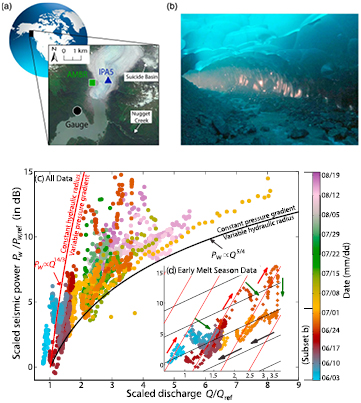
Figure 28. Subglacial water transport generated seismic noise at Mendenhall Glacier, Alaska. (a) Site map, showing the location of (rock-sited) seismograph (AMBR) 50–100 m W of the edge of the glacier and 2 km from the glacier terminus. A nearby gauge at proglacial Mendenhall Lake used for net water discharge monitoring, and a glacier-sited GPS geodetic site (IPA5) were used to monitor glacial motion. (b) Representative photograph of a subglacial conduit (several m in diameter). (c) Scaled short-period (2–5 Hz) seismic velocity power ( , in db) versus scaled discharge (
 ), with time of measurement indicated by the color bar at right, Reference power and discharge are representative of minimum power and minimum discharge. (d) detail of (c) for the early season (early June through early July), showing multi-day excursions interpreted as displaying episodic pressurization of the conduit under constant hydraulic radius (red arrows), followed by depressurization (green arrows). Predicted power law relationships between seismic power and discharge from the conduit-specific formulation of the power law derived in Gimbert et al (2014) for pressurization of a constant-radius conduit and a constant pressure, variable radius, conduit are shown as red and black curves, respectively. Reproduced with permission from Gimbert et al (2016). © 2016. American Geophysical Union. All Rights Reserved.
Download figure:
Standard image High-resolution imageSeismic signals from flowing water generally arise from time-varying forces associated with turbulent flow, applied to surrounding ice or rock boundaries and/or by the seismic coupling of acoustic sources within the fluid. Such processes may include pressure fluctuations due to gravity waves, tractions applied due to frictional/impact interactions between water and topographic features of the channel, and via the seismoacoustic coupling of cavitation events and breaking waves. The theory of seismic wave generation by flowing water is still in development and proposed processes and models still await full development and testing. Under simplifying stochastic and physical assumptions, useful analytic expressions for expected seismic power spectral density have recently been derived for turbulent flow in rivers (Gimbert et al 2014) and in confined englacial channels (Gimbert et al 2016), and have been corroborated with data. Seismic radiation from fluvial systems may also exhibit time-varying response (hysteresis) as the channel is modified by rising and lowering flow levels and as the transportation or disposition of sediment changes, e.g. Schmandt et al (2013). The presence of sediment may create additional and distinct (e.g. in a distinct frequency band) signals via additional traction and/or impact forces generated by transported bed load constituents (Tsai et al 2012, Burtin et al 2016).
9. Future directions in glacial seismology
During the past two decades, synoptic scale observations that have become available due to a range of satellite observations, including altimetry, gravimetry, and InSAR, have revealed large secular trends in the behavior and mass balance of the Earth's cryosphere. However, space-borne observations of the physical processes that control these trends (i.e. calving) are often temporally aliased due to their relatively low temporal sampling (typically greater than once per day). Dense temporal sampling provided by terrestrial based observations, including seismic observations, thus remains essential to understanding the processes and future evolution of the cryosphere. Continued advances in glacial seismology can be expected to be strongly driven by continually improving seismological instrumentation and methodologies, theoretical developments that enhance modeling and hypothesis testing, inversion advances, and new interpretations of seismic observables (e.g. using seismic attenuation as a proxy for temperature, Peters et al (2012)), and by progress in the further identification and directed interdisciplinary study of critical processes affecting the dynamics of glacial systems.
Broadband and short-period seismographs can now be deployed in extreme polar and alpine glacial environments worldwide, and low-Earth-orbit satellite and other real-time data telemetry options are increasingly available (although in some cases remain expensive or draw intractable amounts of power for year-round operation). However, the dynamic surface environment in areas experiencing large degrees of snowfall, ablation, melting, crevassing, calving, and other processes also limits the degree to which stable and recoverable instrumentation can be deployed. Improved capabilities to deploy seismometers in ice boreholes from the near surface to basal, or potentially sub-basal depths, offer exciting prospects to establish more stable and lower noise observational environments. Such deployments enable measurements of seismic wavefields, material properties and, pressure/temperature states in close proximity to seismic sources, including the critical glacial bed environment. A presently evolving new generation of cheaper and easier to deploy seismographs should result in much denser (in some cases functionally spatially unaliased) short-period recordings of the seismic wavefield on glaciers to advance both seismic source and propagation-related studies, e.g. Aster and Simons (2015).
Photogrammetry, satellite and airborne remote sensing, radar, electromagnetic, and other sensing methods will continue to grow in capabilities and importance, both inherently and as multidisciplinary capabilities that may be partnered with seismological studies. Surface, airborne and space-based ice penetrating radar is a key glaciological tool with very wide use in glaciology for surface and internal imaging, e.g. Arcone (2004). Co-evolving advances in instrumentation, and their greater deployment and integration, can be expected to continue to expand understanding of glacial structure and dynamics, and at greater resolution, as greater numbers of multi-observational studies in areas of particular interest can be realized. Larger numbers of focused studies will also be essential to better understand and characterize the general, as opposed to particular, behavior of glacial systems. In addition to focused studies, denser, wider-ranging, and longer duration deployment of seismographs in glaciated regions can be expected to continue to broadly improve understanding of glacially associated seismogenic regions and their seasonal and longer-term evolution. A number of advanced seismic methodologies that have been widely employed in other environments (e.g. in volcano seismology and shallow Earth imaging) currently still await commensurate realization in glaciological applications.
One such promising methodology is the use of ambient or seismic coda correlation for imaging, and/or near-continuous monitoring of distributed seismic properties, e.g. Duputel et al (2009), Zhan et al (2014), Larose et al (2015) and MacAyeal et al (2015). Such methods could provide continuous measurements of the bulk strength and evolution of glacial features. Ambient noise correlation-based methodologies hold great potential for resolving bulk or localized property changes as well as their bounding basal, morainal or other features. Seismological study of mixed rock/snow/ice/permafrost systems, e.g. Overduin et al (2015) and Dafflon et al (2016) will see significant geophysical attention in the context of increased thaw conditions and associated hazards, such as glacial outburst floods. Seismology is also seeing increasingly routine use in the management of snow avalanche hazards, e.g. van Herwijnen and Schweizer (2011) and Pérez-Guillén et al (2016). Subglacial hydrology and sediment properties of glacial systems is similarly primed for greater study, and may be particularly important to the future dynamical behavior of glacial systems with large amounts of surface melt, including Greenland (Walter et al 2014, Mordret et al 2016), and to ice shelves that are responding rapidly to changes in ocean circulation and temperature that can produce underside melt e.g. Paolo et al (2015) and Truffer and Motyka (2016). These systems bear key importance to immediate future sea level rise (Scambos et al 2004, Meier et al 2007, Yi et al 2015). Perhaps the most significant promise of ambient noise correlation seismic methods for imaging is the ability to continuously monitor temporal variability in physical properties, and to thus infer changes in glacier dynamics and/or conditions that drive glacial behavior or integrity, such as fracture growth or englacial water content (Walter et al 2015a). Additionally, emerging results are demonstrating that many passive source techniques developed to image the seismic structure of the solid Earth can be widely applied to glacial environments. Seismic imaging in glacial environments has a long history, e.g. Roethlisberger (1972), but has historically relied on artificial sources such as an explosions or hammer strikes, although recent work has highlighted the viability of on-ice vibroseis sources as well (Hofstede et al 2013). However, active source seismic surveys are often laborious, thus limiting the amount of data can be collected during a field project. Passive seismic imaging that leverages both discrete natural sources as well as the ambient seismic wavefield is a promising avenue for complimenting traditional active source seismic surveys. For example, the rheology of ice is highly dependent on c-axis fabric orientation (Budd and Jacka 1989). As noted in section 2, seismic wave speeds in single crystal ice are strongly anisotropic, being approximately several percent faster for polarizations that are parallel to, as opposed to perpendicular to, the c-axis (Blankenship and Bentley 1987). This makes seismic waves valuably suited for imaging the bulk crystal fabric of glacial ice in regions that lack direct ice core measurements (Horgan et al 2008). Thus, shear waves generated by a microseismic basal event will show differential arrival times (i.e. shear-wave splitting) if the crystalline fabric or layering is highly anisotropic and suitably oriented (Harland et al 2013, Smith et al 2017). Additional information can be inferred about englacial structure (firn depth, fabric, fracture density) by using surface waves generated by shallow events to map depth-dependent seismic velocity structure (Lough et al 2015, Walter et al 2015a, Diez et al 2016).
Active source seismic studies have also shown the importance of subglacial geology to glacial behavior (Blankenship et al 1986, Anandakrishnan et al 1998). While natural or ambient sources will likely never supersede the need for very high frequency ( 100 Hz) seismic imaging of the ice-bed interface (Smith 2007) and other short-wavelength critical features of glacial systems, passive methods, such as horizontal to vertical spectral ratios (Pratt et al 2016, Picotti et al 2017), and receiver function methods, e.g. Chaput et al (2014) and Walter et al (2014), hold promise for enhanced imaging the large-scale (
 100s of meters) sedimentary structure beneath glaciers and ice sheets.
Glacial and regionally sited seismological observations in Greenland and Antarctica are key to constraining mean and spatially varying viscoelastic properties of the crust and mantle at icecap scales. These properties control the rate of glacial isostatic adjustment (GIA) of the solid Earth to ice loading and unloading, which occurs across time scales from years to millennia. Accurate understanding and modeling of GIA is critically important to the dynamic stability of some large glacial systems, such as in West Antarctica, and to the accuracy of space-based or airborne gravimetric, elevation, and other estimations of ice mass change (van der Wal et al 2015) and sea level rise (Bromwich and Nicolas 2010). Mantle-scale seismic tomography is also seeing application to estimating the geothermal heat flow boundary conditions that are important to subglacial melting, frictional, and hydrologic environments (Schroeder et al 2014, An et al 2015, Fisher et al 2015, Heeszel et al 2016, O'Donnell et al 2017). Improved observations and modeling of seismological signals due to englacial and subglacial water transport offer considerable potential for the monitoring and study of the dynamic, and in some cases karst-like, interiors and basal environments of glacial systems. Finally, continuing geophysical studies of Earth's cryosphere, including seismology, will inform structure and dynamic processes investigations of Mars, and for icy bodies elsewhere in the solar system (Cammarano et al 2006, Panning et al 2006, Kofman et al 2010, Vance et al 2016).
Acknowledgments
We thank two reviewers for substantive comments that improved the quality and completeness of this manuscript. The authors acknowledge support from the National Science Foundation for their research, including POLENET, which is supported by NSF Office of Polar Programs grants 0632230, 0632239, 0652322, 0632335, 0632136, 0632209, and 0632185. JPW was also supported by NSF Office of Polar Program grant 1141889. This paper benefited from comments from students attending the 2017 Glacial Seismology Summer School held at Colorado State University, which was sponsored by NSF (POLENET), the Scientific Committee on Antarctic Research (SCAR), the International Glaciological Society (IGS) and the International Association of Cryospheric Sciences (IACS).
Appendix. Seismology fundamentals
Below, we summarize seismological fundamentals relevant to this review article. For much more detailed treatment of elastic wave propagation and seismological principles, we refer the reader to one of the excellent general seismology texts that are available, including (Stein and Wysession 1991, Aki and Richards 2002, Shearer 2006).
A.1. P and S waves in isotropic and homogeneous elastic media
Expressing the strain tensor elements (8) in terms of the displacement vector,  and expanding in terms of displacement terms lead to the general equation of motion for isotropic media, expressed in vector formulation as

Decomposing the displacement field  into the sum of the gradient of a (zero curl) scalar potential and the curl of a (zero divergence) vector potential via a Helmholtz decomposition gives

We can simplify this expression by noting that

and

so that

Grouping the potential terms in (A.5) gives
The left hand side of (A.6) is the gradient of a function of Φ, while the right hand side is the curl of a function of Ψ. Setting the two bracketed terms to a constant separates the elastodynamic equation of motion into two wave equations. Choosing a constant of zero (i.e. no source terms) gives the wave equations

and

that characterize the two fundamental (P and S) seismic body waves in an isotropic, homogeneous elastic medium.
Because wave fields are most often observed in the far field, plane wave modeling is frequently employed for studying seismic phenomena. A harmonic Helmholz potential plane-wave scalar displacement potential is


where  is the vector (propagation direction) wave number. The P wave displacement field due to the displacement potential (A.9) is thus

where  . This is a harmonic displacement disturbance with all displacement in the propagation direction
  and an amplitude proportional to
  . The P wave displacement field thus consists of once-per-wavelength compressions and rarefactions. The dilatation of the P wave as a function of space and time is given by

which does not vary perpendicular to the  direction. Volumetric strain propagating in the P wave is thus caused by shortening in the
  direction.
The corresponding displacement field from a harmonic Helmholtz potential plane-wave vector displacement potential Ψ is


The displacement in the S wave is perpendicular to the propagation direction,  , and the dilatation, consistent with infinitessimal shear strain, is zero everywhere and at all times

so that the S wave propagates solely shear strain.
A.2. Coupling of P, S, and surface waves
A horizontally layered medium of uniform elastic layers is often usefully employed in seismology, Reflection and transmission (scattering) coefficients for like (P–P and S–S) and converted (P-S and S-P) plane seismic waves for this case are readily derivable by matching displacement and traction boundary conditions at media interfaces for ansatz plane harmonic wave solutions (obeying Snell's Law, as dictated by associated wave speeds defined by (12) and (13)). In the case of plane isotropic layers and plane waves, the seismic wavefield can decomposed into two independent wave systems. The first of these wave system is a system of S waves with particle motions that are perpendicular to the ray plane (referred to as SH). The second wave system is the coupled system of P and S waves with particle motions lying within the ray plane (referred to as  ). Seismic transmission and reflection coefficients can be expressed algebraically in closed forms in terms of Snell's law angles and material density and elastic parameters, and a complete set of reflection and transmission coefficient relationships for isotropic media can be found in Aki and Richards (2002). However, in elastically anisotropic media
  and SH are no longer decoupled, and are thus not generally separable in this manner. Transmission and reflection coefficients for VTI media may be found in Graebner (1992), and linearized expressions for more general anisotropic media can be found in Behura and Tsvankin (2009).
An important system of coupled P and S waves is the phenomenon of seismic surface and other boundary waves associated with a free surface or other inhomogeneous interface. Such waves can be theoretically derived as coupled propagating and evanescent components of the wavefield. The interface between the solid Earth and the atmosphere can be practically considered as a free surface under most circumstances, and for horizontally layered media, surface waves can be derived using the stress-free boundary condition and corresponding reflection coefficients for a free surface, e.g. Stein and Wysession (1991). Coupled P and S surface waves polarized in the  (ray) plane are generically referred to as Rayleigh waves, and surface waves comprised of S waves with particle motions perpendicular to the ray plane are generically referred to as Love waves. As with systems of non-evanescent waves, the Rayleigh (P-SV) and Love wave (SH) components of the seismic wavefield are fully decoupled only in the case of horizontally layered isotropic media. Surface waves in layered media will exhibit dispersion, which is commonly utilized for structural inversion on all scales. Surface waves are also preferentially excited by shallower sources, and may serve as a discriminant for depth.
A.3. Seismic sources
Seismic waves are excited when transient forces are applied at the boundaries of or internally within an elastic medium. Important sources in the cryospheric environment include examples of both types. Internal localized (so that they may be approximated by a point) sources within an elastic medium are typically characterized by a second-order seismic moment tensor,  , where they corresponding scalar moment is
The seismic moment tensor elements  represent the relative magnitudes and signs of opposing force couples oriented in the xi directions operating in plane specified by the normal vector xj. Diagonal moment tensor elements thus represent opposing normal forces that are applied normal to principal planes, and off-diagonal elements represent shear couples. Because internal source process (e.g. collapse, explosion, or fault slip) cannot impart a net change in angular momentum, the moment tensor is symmetric. M0 has units of force times distance (i.e. N-m in SI units).
A practically important moment tensor type is that of a double-couple, which describes equivalent force couples corresponding to a slipping mode II (in-plane shear) crack and is thus appropriate for slip on a fault or at a glacier bed. The scalar moment of a double couple source can be usefully calculated as

where A is the slip patch area, d is the average fault slip, and μ is the rigidity of the surrounding elastic medium. Isotropic volumetric expansion (e.g. explosion) and force couple components of a point seismic source can be represented by a diagonal moment tensor. Additionally, single (non-couple) forces, not represented in the moment tensor, can also be important elements of a seismic source characterizations, such as in modeling reaction forces related to the advection of gas or fluid, or gravitational or otherwise externally driven boundary force, such as may occur during glacial calving processes.
Seismic source sizes are commonly reported using magnitude scales, which are calculated from an appropriately scaled logarithmic formula that incorporates geometric spreading and otherwise appropriately corrected seismic amplitude or other robust observables, e.g. Shearer (2006). Magnitude estimates are typically constrained by a network of seismic stations that measure the seismic radiation over an appropriate angular extent. There are many magnitude scales in historical usage, each derived from different observables (e.g. amplitudes of body waves or surface waves within particular period bands). The most physically fundamental magnitude scale is one based on the scalar moment, referred to moment magnitude, which is now in wide general use. For a scalar moment M0 in SI units, the corresponding moment magnitude is given by Hanks and Kanamori (1979)
(A.16) provides reasonable consistency with historic magnitude scales over a wide range of sources sizes, but does not exhibit saturation or other technical problems at very large magnitudes, as can occur with other magnitude scales, e.g. Shearer (2006). For example, fault slip of 0.01 m on a fault plane measuring 100 by 100 m in ice with a medium rigidity characterized as  Pa corresponds to a scalar seismic moment of
  N m and a corresponding moment magnitude of
  .
.
For a general double-couple seismic source representation with  specifying the normal to the fault plane and
  specifying the unit fault slip vector, the moment tensor is given by
Seismic sources induce both near-field (non-propagating, static) and far-field (propagating as elastic waves and transitory) strain within an elastic medium. Near-field strain terms may become important when seismographic or other measurements of strain are recorded very close to a source region and/or for large seismic events, and may best be observed geodetically due to their static and sometimes large-amplitude components (e.g. using GPS or other positional instrumentation). In the more commonly relevant situation for glacial seismology, far-field, case, P and S wave displacement amplitudes will decay due to geometric spreading as the inverse of distance and be proportional to applied force amplitudes for single forces and proportional to the time derivative of applied couple amplitudes (or to the moment rate function in the case of extended time sources) for force couples (Aki and Richards 2002).
The orthogonal eigenvectors of (A.17) are referred to as the  (tension),
  (pressure), and
  (null) axes, and have eigenvalues M0,
  , and 0, respectively. The
  and
and  axes are the centers of the compressional and dilitational quadrants of the P wave radiation pattern from the double couple source (the maximum and minimum P wave amplitude radiation directions). Conversely, the
  axis is the axis of zero radiated P- and S- wave energy, which occurs at the intersection of the fault plane and its (indistinguishable from P wave polarity information) counterpart, the auxiliary plane. The fault and auxiliary planes of a double-couple solution lie at
  to the
  and
and  axes, and the intersection of the fault and auxiliary plane denotes the
  axis (figure A1). Analytic expressions for seismic radiation terms for isotropic media can be found in Aki and Richards (2002).

Figure A1. Schematic depiction the relative amplitudes and medium displacement directions of P and S wave far-field seismic waves (arrows) created by a slipping fault (indicated) embedded within an isotropic elastic medium. The slip vector,  lies in the fault plane and the fault normal,
  lies in the (perpendicular) auxiliary plane, each indicated. The intersection of the fault and auxiliary planes defines the
  axis (which is also orthogonal to the
  and
and  axes). The far-field seismic radiation from an orthogonal fault, slipping in the opposite sense so that the auxiliary and fault planes are interchanged (i.e. by rotating the fault
  about the
  axis and reversing the slip direction), is identical. This fault/auxiliary plane ambiguity can often be resolved with additional seismological observations or from geological/glaciological context (e.g. when it is known that the source is slip on a glacial bed). Adapted from Shearer (2006).
Download figure:
Standard image High-resolution image
Biographies

Richard Aster (PhD Scripps Institution of Oceanography, 1991) is Professor of Geophysics and Department Head of Geosciences at Colorado State University. His work has included multiple field projects and field seasons in Antarctica, working on the Ross Ice Shelf, in multiple locales in West Antarctica, on Mount Erebus, and at South Pole.

J. Paul Winberry (PhD, the Pennsylvania State University, 2008) is a research geophysicist in the Department of Geological Sciences at Central Washington University. His research is focused on glacier physics as well as the interactions between the solid-Earth and ice-sheets. He has conducted field experiments in Antarctica, Greenland, Alaska, and Norway.