
Abstract
The quality of laser wakefield accelerated electrons beams is strongly determined by the physical mechanism exploited to inject electrons in the wakefield. One of the techniques used to improve the beam quality is the density transition injection, where the electron trapping occurs as the laser pulse passes a sharp density transition created in the plasma. Although this technique has been widely demonstrated experimentally, the literature lacks theoretical and numerical studies on the effects of all the transition parameters. We thus report and discuss the results of a series of particle in cell (PIC) simulations where the density transition height and downramp length are systematically varied, to show how the electron beam parameters and the injection mechanism are affected by the density transition parameters.
Export citation and abstract BibTeX RIS

Original content from this work may be used under the terms of the Creative Commons Attribution 3.0 licence. Any further distribution of this work must maintain attribution to the author(s) and the title of the work, journal citation and DOI.
1. Introduction
Laser wakefield acceleration (LWFA) [1–3] of electron beams is one of the most promising physical mechanisms to overcome the accelerating gradient limitations of conventional accelerators. The electromagnetic fields in the wake of an intense laser pulse propagating in an underdense plasma can sustain magnitudes of hundreds of GV/m [4–7], allowing to produce femtoseconds-length [8] electron beams with GeV energy [9]. Currently, the quality of electron beams produced through LWFA has been proven to be suitable for radiography [10, 11], ultrafast electron diffraction [12] and assessed as potentially suitable for applications in radiotherapy [13, 14]. Applications of conventionally accelerated beams also include research tools with more strict requirements on the beam quality, such as free electron lasers (FELs) [15, 16], for which one needs to improve quality figures such as energy spread, emittance and divergence. The beam quality in LWFA is tightly related to the mechanism used to inject the electrons that are then accelerated. Such an issue motivates the interest in the study of various injection techniques [3] such as colliding pulse injection [17, 18], ionization injection [19–22], density tailoring injection schemes [23–27] or hybrid techniques [28] to obtain progressively improved beam qualities.
An easy-to-implement scheme to trigger electron injection in a laser wakefield accelerator consists of creating a sharp density transition in the propagation direction of the laser pulse in a gas jet [25, 26]. The resulting plasma density profile shows a rising ramp followed by a sharp downramp. After the downramp, the wakefield electron cavity, or 'bubble', behind the laser pulse increases its size, trapping some of the electrons from the density transition. Thaury et al [28] report electron beams of charge 1 pC produced through this technique, accelerated to energies about 100 MeV, with lowest energy spread 10 MeV on 10 consecutive shots; those beams were obtained with plasma density  cm−3 at the density profile center, laser pulse with peak intensity in vacuum
  W/cm2, pulse length and transverse size near to those used for the simulations in this work. The final beam parameters can be tuned by changing the position, length and height of the density transition peak in the plasma [26]. This injection scheme has been experimentally investigated [25, 26] and the effects of the transition downramp length in the density downramp injection scheme have been examined thoroughly in [27]. However, no systematic investigation is present in the literature on the effects of the downramp length and the transition height in a density profile with a spike-like profile density, in the literature called shock-front [26, 28]. Our results are consistent with those found in [27].
To further assess possibilities, limits and scaling laws of the density transition injection scheme, we present in this work the results of a series of simulations where the density transition characteristics are systematically changed and discuss how they influence the injected electron beam quality.
The article is organized as follows. In the second section we describe the parametric numerical study. In the third section we show the injected beam parameters, discussing their variation with the height and the length of the density transition downramp. In the fourth section additional considerations on the distribution in the transition downramp of the injected electrons are reported.
2. Parametric numerical study
To investigate the dependence on the density transition characteristics of the electron beams obtained through density transition injection, a parametric scan was performed with the particle in cell (PIC) code CALDER-CIRC [29]. The simulations were performed in quasi-cylindrical geometry, i.e. the electromagnetic fields are decomposed in azimuthal modes with respect to the laser propagation direction, while the simulated macroparticles move in the 3D Cartesian space [29]. The results reported in this work have been obtained retaining the first two azimuthal modes. We chose a mesh resolution 
 and
and 
 in the longitudinal and radial direction, respectively, with integration timestep
 , where
  is the laser central frequency. The results shown in the following have been obtained with 50 particles per mesh cell. We considered driver laser pulse parameters based on the Ti:Sa laser system of Salle Jaune at Laboratoire d'Optique Appliquée (LOA), i.e. wavelength
  μm, FWHM duration 28 fs. In the simulations the pulse, linearly polarized along the y direction, is focused to a waist size
  μm at the entrance of an already ionized underdense plasma, whose longitudinal profile is depicted in figure 1. After a linear upramp of length
  μm until the position ztp of the density transition peak, the electron density ne of the plasma drops linearly for a length Ldown to the value of
  cm−3. The driver laser pulse is injected from z = 0 μm, directed towards the positive z direction. After the downramp, the density profile has a plateau of constant density n0. The density transition at the beginning of the plasma channel has a peak of electron density of value Kn0, where K is the ratio between the density transition peak density and the plateau density. The normalized potential of the laser pulse at the waist is a0 = 2.5, corresponding to a total energy E = 0.9 J. The considered laser pulse parameters and plateau density yield a ratio between the total pulse power and the critical power
 PW at waist for relativistic self-focusing [30] equal to 3, which causes a slight self-focusing during the propagation, as shown in figure 2. As the laser pulse passes through the density transition, electrons are injected before being accelerated in the plateau region. The injected electron beam is then accelerated along the plateau by the laser wakefield. For K = 1, i.e. in absence of a sharp density transition in the plasma profile before the plateau, the mentioned self-focusing of the laser (see figure 2) and the consequent change in the size of the bubble do not trigger self-injection. Varying K and Ldown within the intervals considered by our study, the laser propagation remains almost identical to the one showed in figure 2. The only difference between the various simulations corresponding to the considered density transition parameters is a slight variation of the peak a0 during the propagation, with a maximum difference between the simulations smaller than 5%.
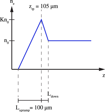
Figure 1. Plasma density profile used in our study. The laser propagates in the positive z direction. The density transition peak is located at  μm. Our diagnostic point for the beam quality parameters corresponds to the time when the laser pulse reaches z = 1 mm.
Download figure:
Standard image High-resolution image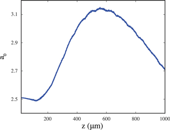
Figure 2. Evolution of laser maximum vector potential a0 during the propagation in the plasma, without a sharp density transition before the density plateau ( .
.
Download figure:
Standard image High-resolution imageOur investigation included the systematic variation of the density transition height ratio, represented by K, and the density transition downramp length Ldown within experimentally feasible intervals [26], i.e. ![$K=[1.2,1.5]$](https://content.cld.iop.org/journals/0741-3335/59/8/085004/revision2/ppcfaa717dieqn18.gif) and
and ![${L}_{{\rm{down}}}=[10,50]$](https://content.cld.iop.org/journals/0741-3335/59/8/085004/revision2/ppcfaa717dieqn19.gif) μm.
μm.
3. Electron beam quality
In this section, we report the results of 15 simulations, representing combinations of ![$K=[1.2,1.3,1.5]$](https://content.cld.iop.org/journals/0741-3335/59/8/085004/revision2/ppcfaa717dieqn20.gif) and
and ![${L}_{{\rm{down}}}=[10,20,30,40,50]$](https://content.cld.iop.org/journals/0741-3335/59/8/085004/revision2/ppcfaa717dieqn21.gif) μm. We did not observe any injected charge for K = 1.1. For each simulation, the parameters of the resulting beam are evaluated when the laser pulse arrives at z = 1 mm.
μm. We did not observe any injected charge for K = 1.1. For each simulation, the parameters of the resulting beam are evaluated when the laser pulse arrives at z = 1 mm.
The total charge of the beam is reported in figure 3. Each point represents one of the 15 simulations. The different curves correspond to different density transition height ratios: red curve K = 1.2, green curve K = 1.3, blue curve K = 1.5. Higher density transitions result in a higher number of trapped electrons, longer density transitions instead yield a lower amount of trapped charge (this last trend was also found in [27]) for downramp injection. The total amount of injected electrons increases more quickly with K than with Ldown. The reasons for these trends are multiple. First, an injection stage with high density contains more electrons available for injection. Second, the amount of injected charge is also related to the speed of bubble size expansion [31]. The bubble size scales as the plasma wavelength  , where me is the electron mass,
  the vacuum permittivity, e the electron charge,
 the electron density at position z in the downramp; thus the relative bubble size increase rate scales as

where  is the plasma wavelength in the plateau,
  the normalized electron density. Figure 4 shows the values of
  for each value of K and Ldown of our simulations. Especially for
  μm, the bubble expansion rate increases more by increasing K than by decreasing Ldown. In this particular injection scheme, the bubble size expansion is equivalent to a decrease in the wake phase velocity, due to the inhomogeneity of the plasma density [23].

Figure 3. Variation of the beam injected charge with the density transition height K and downramp length Ldown. The reported energy is evaluated  μm after the density transition peak. Each point represents the result of one simulation.
Download figure:
Standard image High-resolution image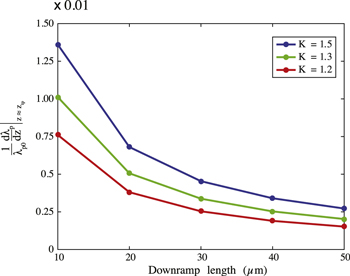
Figure 4. Variation of the relative plasma wavelength expansion speed  with the density transition height K and downramp length Ldown. The reported
  is evaluated at the density transition peak position
  . Each point represents the value computed for one simulation.
Download figure:
Standard image High-resolution imageThe duration of the resulting beam, reported in figure 5, shows variation trends analogous to those of the charge (see figure 3). The bunch length decreases with Ldown and increases with K. From figure 5 it can also inferred that the bunch length is more sensitive to changes in K than to changes in Ldown: fixing the density transition ratio to K = 1.2 the maximum variation is found, i.e. 35% passing from  μm to
μm to  μm, with a rate approximately linear; instead, passing from K = 1.2 to K = 1.5 with the same
  , the electron beam becomes 80% longer. To qualitatively explain such behavior, properly chosen consecutive snapshots of the electron density during the injection process are reported in figures 6 and 7. The snapshots in figure 6 follow the injection in two simulations with K = 1.3 and two different values of Ldown, i.e. 20 μm, and 50 μm. With both values of Ldown, since the density transition height is the same, the bubble initial size and position is the same when its tail is at
  μm (or
  μm in the left panels); in the following, we set the time of this occurrence as t = 0 fs. The density decrease in the downramp causes the bubble size increase, or equivalently the decrease in the wake phase velocity, triggering injection. In the simulation with the smallest Ldown, the bubble size reaches earlier a larger size, due to the higher bubble expansion rate (see figure 4). In this simulation the injection process is already started at t = 63 fs, while in the simulation with the longer Ldown the laser pulse has not completely passed the end of the downramp and the injection is not at the same stage (central panels). At t = 1032 fs (right panels) the injection has already ended in both the simulations. From this qualitative picture it can be inferred that the beam length decreases with Ldown due to the difference in the bubble expansion rate, or equivalently in the reduction of the wake phase velocity, which affects the injection timing. Analogously, also the increase of the beam length with K can be related to the bubble size change. To show this effect, the snapshots in figure 7 follow the injection in two simulations with
  μm and two different values of K, i.e. 1.3 and 1.5. The bubble tail, from which the head of the beam is injected, is more advanced with the higher density transition (bottom left panel) at time t = 0 fs, when it has reached the density peak in the case with K = 1.3 (top left panel). After the end of the injection process (right panels), the tail of the bubble, and thus the tail of the beam, is located in a slightly more advanced position in the case with lower K, due to lower beamloading. These differences in the bubble size in the various stages of the injection process contribute to a difference in the final beam length.
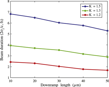
Figure 5. Variation of the beam duration (evaluated as twice the rms length in time) with the density transition height K and downramp length Ldown. The reported duration is evaluated  μm after the density transition peak. Each point represents the result of one simulation.
Download figure:
Standard image High-resolution image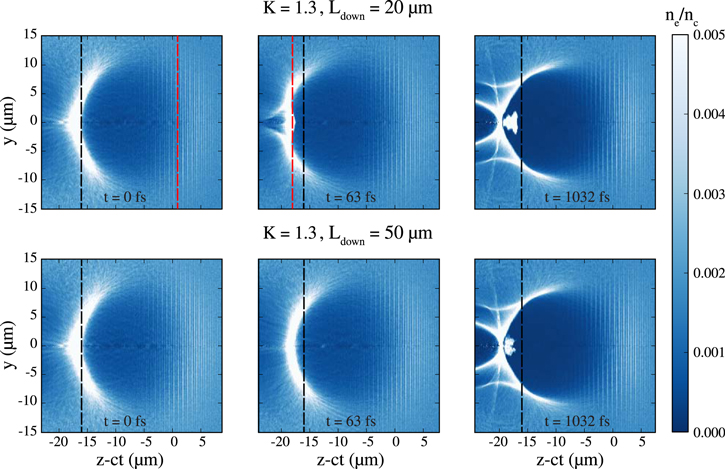
Figure 6. Injection process with a density transition ratio K = 1.3, shown with snapshots of the electron density at time t = 0 (left panels), t = 63 fs (central panels), t = 1032 fs (right panels). The tail of the wake bubble is at the position of the density transition peak ( μm) at t = 0 fs. Top panels show a simulation with
  μm, while the bottom panels show a simulation with
  μm. The dashed black lines are drawn at a constant z − ct position, to help evaluating the longitudinal deformation of the bubble. The dashed red lines mark the end of the downramp.
Download figure:
Standard image High-resolution image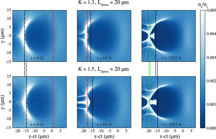
Figure 7. Injection process with a shock ratio  μm, shown with snapshots of the electron density at time t = 0 (left panels), t = 63 fs (central panels), t = 1032 fs (right panels). The tail of the wake bubble is at the position of the density transition peak (
 μm) at t = 0 fs in the top panels, which show a simulation with
  the bottom panels show a simulation with K = 1.5. The dashed black lines are drawn at a constant z − ct position, to help evaluating the longitudinal deformation of the bubble. The dashed green lines in the right panels are drawn to help evaluating the longitudinal bubble size after the end of injection. Both the dashed black and green lines have been prolonged to highlight the different positions of the wake bubble tails for different values of K. The dashed red lines mark the end of the downramp.
Download figure:
Standard image High-resolution imageFor future applications as FEL radiation generation, also the transverse quality of injected beams is of paramount importance [15, 16]. In figure 8, the beam normalized emittances  (
( are respectively the standard deviation in transverse position and transverse momentum,
  is the correlation between transverse position and transverse momentum) in the planes
  at the diagnostic point are reported. The emittance globally shows a symmetry between the transverse planes and a slight decrease with longer downramps. In all our simulations, the beam divergence in both directions is bound within 5 and 9 mrad, the transverse rms size
  does not exceed 1.5 μm.
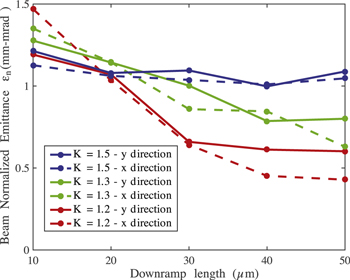
Figure 8. Variation of the beam normalized emittance with the density transition height K and downramp length Ldown. The reported emittance is evaluated  μm after the density transition peak. Each point represents the result of one simulation.
Download figure:
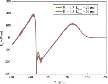
Standard image High-resolution imageThe mean energy of the beam, shown in figure 9, is higher with a lower density transition, e.g. K = 1.2, and increases with the downramp length. For all the considered density transition heights, keeping fixed K, the beam energy increases with the downramp length approximately by 10 MeV for each increase of 10 μm in Ldown. One reason of this behavior is related to the injection process: when electrons start to be trapped, they are located at a certain distance from the laser pulse, in a phase of the wake where the accelerating field is high; after the bubble has reached its final size, the same distance from the laser pulse corresponds to a phase with lower accelerating field. The electrons injected at a later stage instead are located in a phase that has already reached a steady-state configuration with a high accelerating field. Longer beams tend thus to have a lower mean energy due to the lower energy of the early-injected electrons. In addiction, beam loading strongly deforms the accelerating field to which the trapped electrons are subject, influencing them for all the accelerating stage. To highlight the beam loading effect on the accelerating field, figures 10 and 11 report the longitudinal electric field on the propagation axis when the laser pulse is at position  μm. In figure 10, the longitudinal electric field is reported for different values of the density transition height keeping fixed the downramp length to
  μm, showing that with increasing values of K, due to a higher charge (see figure 3), the waveform is much more deformed and the accelerating field experienced by the beam is lower. Instead, keeping fixed K, longer ramps yield a lower injected charge and thus a less-pronounced beam loading, as shown in figure 11 for K = 1.3. Consistently with these two factors affecting the beam energy, a negative correlation can be found between the beam energy and charge and between beam energy and duration. Negative correlation between energy and charge has been observed also with the colliding pulse injection scheme [32] and in simulations of downramp injection [27].
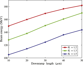
Figure 9. Variation of the beam energy with the density transition height K and downramp length Ldown. The reported energy is evaluated  μm after the density transition peak. Each point represents the result of one simulation.
Download figure:
Standard image High-resolution image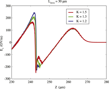
Figure 10. Longitudinal electric field Ez on laser propogation axis for different values of K, with  μm, at the time when the laser pulse has reached position
  μm.
μm.
Download figure:
Standard image High-resolution image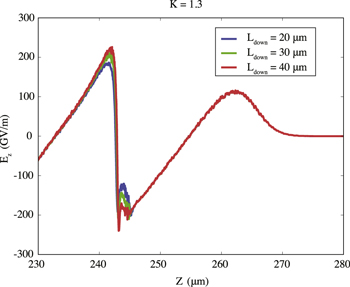
Figure 11. Longitudinal electric field Ez on laser propogation axis for different values of Ldown, with K = 1.3, at the time when the laser pulse has reached position  μm.
μm.
Download figure:
Standard image High-resolution image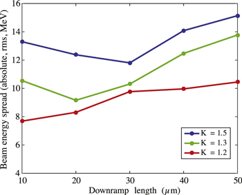
Figure 12. Variation of the beam rms energy spread with the density transition height K and downramp length Ldown. The reported energy spread is evaluated  μm after the density transition peak. Each point represents the result of one simulation.
Download figure:
Standard image High-resolution imageFigure 12 reports the rms energy spread of the beam. In all our simulations, it is lower than 15 MeV, increasing with K as the beam charge and duration.
For convenience, the previously shown beam parameters are reported in table 1.
Table 1.
Variation of the beam charge Q, duration  , transverse normalized emittance
  , energy E, energy spread
  with the density transition height K and downramp length Ldown. The reported quantities are evaluated
  μm after the density transition peak.
| K | Ldown (μm) | Q |
 (fs) (fs) |
 (mm-mrad) (mm-mrad) |
E (MeV) |
 (rms, MeV) (rms, MeV) |
|---|---|---|---|---|---|---|
| 10 | 28.1 | 2.44 | 1.2−1.5 | 150 | 7.7 | |
| 20 | 17.4 | 2.32 | 1.1−1.0 | 160 | 8.3 | |
| 1.2 | 30 | 7.6 | 2.03 | 0.6−0.6 | 169 | 9.8 |
| 40 | 2.6 | 1.77 | 0.6−0.4 | 176 | 10.0 | |
| 50 | 0.9 | 1.68 | 0.6−0.4 | 182 | 10.4 | |
| 10 | 48.4 | 3.94 | 1.4−1.4 | 128 | 10.5 | |
| 20 | 39.0 | 3.69 | 1.4−1.4 | 138 | 9.1 | |
| 1.3 | 30 | 26.1 | 3.52 | 1.2−1.1 | 150 | 10.3 |
| 40 | 16.2 | 3.17 | 1.0−1.1 | 160 | 12.8 | |
| 50 | 10.6 | 2.30 | 0.7−0.6 | 170 | 13.8 | |
| 10 | 79.1 | 6.83 | 1.3−1.3 | 105 | 13.3 | |
| 20 | 75.5 | 6.49 | 1.2−1.2 | 114 | 12.4 | |
| 1.5 | 30 | 58.7 | 6.03 | 1.2−1.2 | 124 | 11.8 |
| 40 | 46.3 | 6.77 | 1.2−1.2 | 136 | 14.1 | |
| 50 | 38.0 | 5.29 | 1.1−1.1 | 144 | 15.1 | |
4. Initial distribution of the injected electrons
Further information on the injection process can be inferred looking at the initial positions of the injected electrons. The charge distributions with respect to the initial positions z0 and x0 of the injected electrons from four representative simulations (corresponding to  and
and  μm) are shown in figure 13. The average value and rms spread of such distributions are reported in table 2.
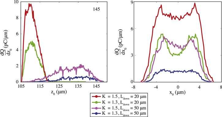
Figure 13. Left panel: Charge distribution  with respect to the initial longitudinal coordinate z0 of the injected electrons in the simulations corresponding to
  and
and  μm. Right panel: Charge distribution
  with respect to the initial transverse coordinate x0 of the injected electrons in the simulations corresponding to
  and
and  μm.
μm.
Download figure:
Standard image High-resolution imageTable 2.
Average  and rms spread
  of the charge distribution with respect to the initial coordinates z0 and x0 of the injected electrons in the simulations corresponding to
  and
and  μm. The reported charge distributions have been evaluated considering the initial positions of the particles; to highlight this, the axes have been relabeled as z0, x0.
| K | Ldown (μm) |
 (μm) (μm) |
 (μm) (μm) |
 (μm) (μm) |
|---|---|---|---|---|
| 1.5 | 20 | 110.8 | 2.9 | 3.0 |
| 1.3 | 20 | 111.3 | 2.9 | 2.9 |
| 1.5 | 50 | 132.3 | 7.9 | 2.7 |
| 1.3 | 50 | 133.6 | 7.2 | 2.6 |
As can be seen from figure 13 (left panel), the injection starts from the density transition peak ( μm) and ends some microns before the end of the downramp. The two charge distributions for
  μm are very similar longitudinally, except for a different peak due to the higher number of injected electrons in the case with K = 1.5. Their longitudinal rms spread
  is essentially the same, while their longitudinal average value
  is smaller by 0.5 μm for K = 1.5. In the case of longer downramps, the longitudinal initial distribution of the injected electrons is centered further from the density peak, since the enlarging bubble traps a larger fraction of electron as the laser propagates in the downramp, and it is slightly more spread for a higher density transition.
Transversely (figure 13, right panel), with a given Ldown, density transitions with different K yield initial charge distributions of injected electrons that are very similar apart from the peak value: passing from K = 1.3 to K = 1.5 enlarges  only by 4%. Instead, a greater enlargement is obtained keeping fixed K, but decreasing Ldown: passing from 50 μm to 20 μm enlarges
  transverse by 11%. Intuitively, a greater difference between the bubble transverse size after and before the density transition triggers injection in a region transversely broader.
It is interesting to compare the cases with K = 1.3,  μm and K = 1.5,
  μm, both yielding beams with
  pC. Being the total amount of charge the same, a similar beamloading (see figure 14) is obtained and thus an energy with a difference only equal to 4% after
  μm. But, although their initial electron distribution is transversely similar in peak, extent and qualitative shape, their longitudinal distributions are visibly different, resulting in a difference in duration higher at least by 40%. This leads to different absolute energy spreads, 9 MeV and 15 MeV, respectively. Analogous similarities and differences in the beam quality parameters can be found in other cases with nearly equally charged beams shown in the previous section, e.g. K = 1.2,
  μm and K = 1.3,
  μm. From this qualitative consideration it can be inferred that among bunches with a given charge obtained through this injection scheme, those produced with a shorter density transition tend to have a higher quality in energy spread and duration.
Figure 14. Longitudinal electric field Ez on axis at the time when the laser pulse has reached position  μm in the simulations with K = 1.3,
  μm and K = 1.5,
  μm. In these two simulations, beams with same charge (
 pC) are injected.
Download figure:
Standard image High-resolution image
5. Conclusions
In this paper, we showed the results of a series of quasi-cylindrical PIC LWFA simulations of electron beams produced through density transition injection, feasible e.g. with a blade inserted in a gas jet. Our analysis highlights the physical mechanisms of the density transition injection that influences the final beam characteristics. We discussed how the beam quality parameters after  from the density transition vary with the density transition height and downramp length. We found that longer and lower density transitions, due to a lower number of electrons available for injection and to the lower rate of wake bubble size increase, yield beams with lower charge, which causes a lower beamloading and thus a negative correlation between the final beam charge and energy. We have also shown how the injection process influences the bunch length, tightly related to the evolution of the bubble size and thus to the density transition profile parameters. With the laser pulse used for our analysis, beams with length shorter than 10 fs, energy higher than 100 MeV reached in less than 1 mm, emittance lower than 1.5 mm-mrad and charge variable up to 80 pC can be envisaged in principle.
Acknowledgments
The authors acknowledge the support by the European Union's Horizon 2020 research and innovation program under grant agreement EuPRAXIA No. 653782 and X-Five ERC project, contract No. 339128.