
Abstract
Objective. Measuring the respiratory signal from a video based on body motion has been proposed and recently matured in products for contactless health monitoring. The core algorithm for this application is the measurement of tiny chest/abdominal motions induced by respiration (i.e. capturing sub-pixel displacement caused by subtle motion between subsequent video frames), and the fundamental challenge is motion sensitivity. Though prior art reported on the validation with real human subjects, there is no thorough or rigorous benchmark to quantify the sensitivities and boundary conditions of motion-based core respiratory algorithms. Approach. A set-up was designed with a fully-controllable physical phantom to investigate the essence of core algorithms, together with a mathematical model incorporating two motion estimation strategies and three spatial representations, leading to six algorithmic combinations for respiratory signal extraction. Their promises and limitations are discussed and clarified through the phantom benchmark. Main results. With the variation of phantom motion intensity between 0.5 mm and 8 mm, the recommended approach obtains an average precision, recall, coverage and MAE of 88.1%, 91.8%, 95.5% and 2.1 bpm in the day-light condition, and 81.7%, 90.0%, 93.9% and 4.4 bpm in the night condition. Significance. The insights gained in this paper are intended to improve the understanding and applications of camera-based respiration measurement in health monitoring. The limitations of this study stem from the used physical phantom that does not consider human factors like body shape, sleeping posture, respiratory diseases, etc., and the investigated scenario is focused on sleep monitoring, not including scenarios with a sitting or standing patient like in clinical ward and triage.
Export citation and abstract BibTeX RIS

Original content from this work may be used under the terms of the Creative Commons Attribution 4.0 licence. Any further distribution of this work must maintain attribution to the author(s) and the title of the work, journal citation and DOI.
1. Introduction
Cameras enable contactless respiration monitoring by measuring subtle respiratory motions from a human body (chest or abdomen). Monitoring of respiration rate is ubiquitous in a video health monitoring system, as it is one of the most important vital signs to indicate a person's health state (Bartula et al 2013). Changes in spontaneous respiratory rate may provide early indications of physiological deterioration or delirium of a patient (Folke et al 2003, Brochard et al 2012), while the average respiratory rate can provide insights into a person's well-being (e.g. sleep quality) (Long et al 2014). The camera is a versatile sensing tool that can potentially be used in a broad range of healthcare applications for health monitoring (Antink et al 2019). Camera-based monitoring has many benefits as compared to contact-based measurement, such as capnography, electrical impedance tomography, accelerometer sensors, respiratory inductive plethysmography and structured-light plethysmography. It reduces direct mechanical contact between sensors and skin and thus eliminates the interaction with the (fragile) skin and potential infection/contamination (e.g. in COVID-19 testing) caused by contact sensors. It also increases the comfort of users and simplifies the personnel workflow, making it more suitable for long-term and continuous monitoring (24/7) as typical in clinical care units or assisted-living homes.
Camera-based respiration measurement has been extensively studied in the last decade (AL-Khalidi 2011, Bartula et al 2013, Lukáč et al 2014, Alinovi et al 2015, Ostadabbas et al 2015, Massaroni et al 2018), and recently has matured in products, such as baby monitoring (Jorge et al 2017), sleep monitoring (Nochino et al 2017), Vital Signs App for hand-held monitoring (Philips 2011), VitalEye for respiratory triggering and gating in Magnetic Resonance Imaging (Philips 2018), etc. Behind these applications, extensive research was carried out in developing hardware setups and software algorithms for camera-based respiration monitoring. Not aiming at a comprehensive literature review, we mention a couple of recent studies in this domain before establishing the research objective of this paper. A review of current advances and systems in contactless optical imaging based respiratory assessment is given in (Rehouma et al 2020), where strengths and limitations of different imaging modalities (e.g. depth senor, CCD camera, radar, LiDAR, stereoscopy) were highlighted in different environments and settings. Beyond visible and infrared wavelengths, feasibility of using Terahertz wavelength for respiration monitoring was also shown (Berlovskaya et al 2020) but it requires a dedicated imaging setup. Additionally, the electromagnetic signals from higher wavelength (lower frequency) range like radio-frequency waves (e.g. Doppler radar based (Lee et al 2014, Pramudita and Suratman 2021), WiFi based (Liu et al 2015, Zeng et al 2019)) and the micro-signals of mechanical waves (e.g. acoustic or sonar based (Wang et al 2018, 2021)) have been used for contactless respiration measurement. Although these are different from optical based measurement and mostly discussed in the wireless sensing community, we foresee a potential of fusing different contactless sensing modalities and a cross-fertilization between two communities (i.e. computer vision and wireless sensing) leading towards multi-modal contactless health monitoring.
Focusing on camera-based monitoring, three different modalities are generally used to measure the respiratory signal from a video camera: motion-based (respiratory motion at chest/abdomen) (Bartula et al 2013, Janssen et al 2015, Rocque 2016, Wiede et al 2017), thermography-based (airflow-exchange induced temperature changes at nose/mouth) (Pereira et al 2015, 2018, Jagadev and Giri 2020), and photoplethysmography-based (respiration modulated blood volume changes at a peripheral living-skin) (Mirmohamadsadeghi et al 2016, Iozza et al 2019, Luguern et al 2021). Among these three principles, the motion-based modality receives most attention in research and application due to its simplicity and applicability, i.e. it does not require dedicated/costly cameras, and has less restrictions on the features of sensors and environment (e.g. lighting conditions) as required by camera photoplethysmography (camera-PPG) (Wang 2017). A regular RGB/monochrome camera (e.g. webcam, IP camera, CCTV camera or mobile phone camera) suffices as a motion sensor for respiration measurement. Not restricted to 2D cameras, depth cameras (e.g. time-of-flight (Penne et al 2008) or structured light (Makkapati and Rambhatla 2016)) and laser Doppler vibrometer (Scalise et al 2011) were used to enhance the sensitivity of respiration measurement in a different optical manner (e.g. in 3D space). The benchmark of three video-based respiration measurement modalities (i.e. RGB, depth and thermal cameras) in (Mateu-Mateus et al 2021) shows that depth and RGB cameras present equally high agreements with the reference (i.e. no statistical difference in between), suggesting that a regular RGB camera may attain promising performance of respiration monitoring. Here we particularly mention that due to attractive properties of the motion-based approach, a couple of thermography-based studies (Bennett et al 2017, Lorato et al 2020, Jakkaew and Onoye 2020) also exploited motion cues in addition to nostril airflow for respiratory assessment. A series of end-to-end solutions were developed for real-time systems and prototypes (Janssen et al 2015, Reyes et al 2016, He et al 2017, Braun et al 2018, Massaroni et al 2018, Lee et al 2021),and, more recently, AI-based solutions (using convolutional neural networks (Brieva et al 2020, Zhan et al 2020, Hwang and Lee 2021, Földesy et al 2021)) were proposed to learn the respiration extraction from labeled training data, though the results reported in (Zhan et al 2020) raised the question whether learning-based approaches can actually improve conventional approaches like optical flow.
Delving deep into the motion-based respiration monitoring, the typical video processing chain can be depicted in three steps: Region of Interest (RoI) detection, motion estimation, and respiratory signal/rate construction. We consider the second step (motion estimation) as the core of processing, while the first and last steps are front and end processes that can be achieved by leveraging generic and existing tools in video and signal processing. Pilot studies in our lab including the present study convinced us that the primary challenge for respiratory motion estimation is the sensitivity to tiny motions. We consider it is important that a respiratory algorithm is sensitive enough to capture the subtle movement induced by inhaling and exhaling at the level of sub-pixel distance. It determines the fundamental behavior of a monitoring system. We note that different from camera-PPG where motion-robust heart-rate monitoring can be achieved by proper design, motion-robust respiration monitoring is much more difficult as motion is the primary information source for the respiration. Thus, other motions like shaking of the body limbs will fundamentally form a disturbing factor. Even for contact-based measurement like using chest belt or accelerometer, it is difficult to measure respiratory signal accurately during body movement; for that purpose other modalities with different measurement principles (e.g. thermography (Pereira et al 2015) that measures respiratory flow induced nostril temperature changes) should be considered.
Regarding the core algorithms for respiratory motion extraction, various approaches (Bartula et al 2013, Janssen et al 2015) have been proposed, which are mainly based on the essence of optical flow (Lucas and Kanade 1981, Lucas 1984) and cross-correlation (Guizar-Sicairos et al 2008, Sarvaiya et al 2009). These proposals have been prototyped and validated on real human subjects, including in clinical trials. However, we consider a model for interpreting the principles of core algorithms combined with a quantifiable benchmark involving detailed control of the respiration-specific challenges to be valuable for the field, especially for understanding fundamental behaviors and boundary conditions of this measurement. To this end, we designed a phantom with controllable parameters and challenge factors to investigate the performance and boundary conditions for motion-based respiratory signal extraction, i.e. the phantom is created by a motor with programmable amplitude, frequency and shape for its motion signals. To explore the essence of core respiratory algorithms, we propose a model to investigate the motion estimation strategies (cross-correlation and optical flow) and spatial representations (different profiles) that are essential for this measurement. Six core algorithms are derived from the model and plugged into a fixed and automatic RoI framework, respectively, for understanding the promises and limitations of different algorithmic components. Finally, a new approach derived in this study is recommended based on the benchmark and analysis. The major difference between our recommendation and earlier methods (Bartula et al 2013, Janssen et al 2015) is that it is designed for extracting subtle motions in the sub-pixel level rather than estimating general motions induced by body movement. The sensitivity to tiny respiratory motion is particularly emphasized by our approach, as shown in both the way of processing and benchmarking results.
The remainder of this paper is structured as follows. In section II, we introduce the phantom study (setup and experimental protocol). In sections III–IV, we introduce the model proposed for respiratory motion extraction and the core algorithms derived from the modeling. In sections V and VI, we evaluate and discuss the core algorithms via the phantom benchmark. Finally, in section VII, we draw the conclusions.
2. Phantom setup and measurement
2.1. Phantom setup
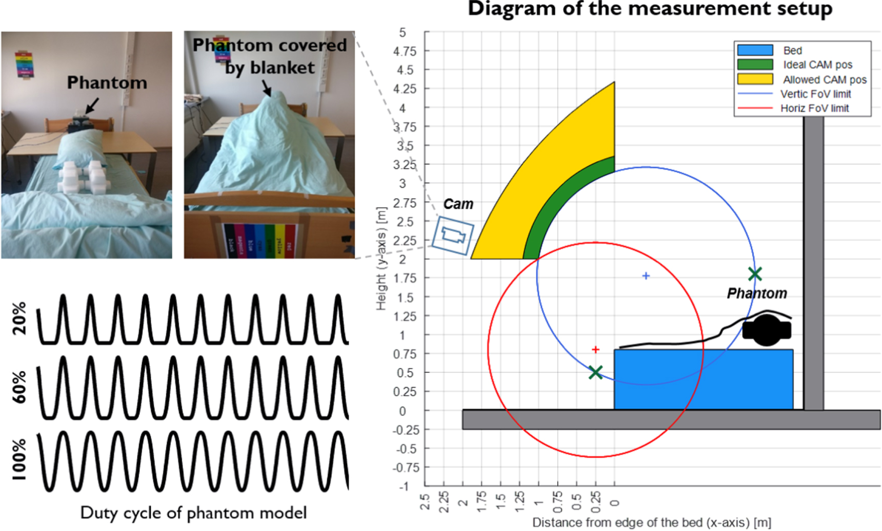
The phantom study was conducted in a lab environment that simulates the scenario of sleep monitoring. Figure 1 illustrates the setup: a physical phantom model that generates respiration-like motion signals was positioned on the upper part of the bed and covered by a blanket to mimic a sleeping person. A camera was mounted on a tripod that is 1.8 m in front of the bed with 2 m height to record the scene.

Figure 1. The diagram of different components in the phantom setup, simulating the scenario of sleep monitoring. A programmable phantom motor, placed at the pillow side of the bed, is used to generate respiratory motion signals with controlled characteristics. The phantom is covered by a blanket to mimic a sleeping person. The green and yellow areas denote the ideal and allowed camera positions for the monitoring of the bed. The red and blue circles denote limit of field of view for the camera in horizontal and vertical directions. The images captured in the view of camera and the respiratory signals generated with different duty cycles are exemplified in the figure.
Download figure:
Standard image High-resolution imageFor the camera sensor, we used the ON Semiconductor MT9P006, which is a 1/2.5 inch CMOS active-pixel digital image sensor. It features low-noise CMOS imaging technology that achieves near-CCD image quality (based on Signal-to-Noise Ratio (SNR) and low-light sensitivity) while maintaining the inherent size, cost, and integration advantages of CMOS. When making video recordings, all auto-adjustment functions of the camera (e.g. auto-focus, auto-gain, auto-white-balance, auto-exposure) were switched off. The videos were recorded in an uncompressed monochrome format (with 480 × 360 pixels, 8 bit depth) at a constant frame rate of 15 frames per second (fps). The relatively low image resolution is intended for investigating the challenging conditions of respiratory monitoring in practical settings with embedded devices and implementation (e.g. products based on edge computing).
The study is aimed at investigating and quantifying the motion sensitivity of core respiratory algorithms. We used a programmable motor to generate phantom motion signals where the signal characteristics (i.e. amplitude, frequency and shape) can be controlled and quantified. A broad range of breathing amplitudes and frequencies (e.g. shallow to deep and slow to fast breathing) were simulated, considering adult and neonatal breathing. A realistic setting for the minimum chest/abdominal excursion in spontaneous breathing was not determined, though (Adedoyin et al 2012) reported that a thoracic chest expansion can be as low as 2 mm.
We mention that the approach of using a respiratory phantom was proposed by (McDuff et al 2020, Wang et al 2020), but in contrast to the approach here, these studies deploy virtual/digital models. Specifically, (Wang et al 2020) used the depth camera to measure respiratory signal from the human body and then a Gate Recurrent Unit (GRU) network to classify different respiratory patterns. In order to train the GRU network, (Wang et al 2020) developed a digital Respiratory Simulation Model to generate abundant training data, which are 1-dimensional signals with different respiratory patterns. (McDuff et al 2020) used Avatars generated from digital facial appearance models and physiological data to synthesize videos to train the network for vital signs measurement. In comparison, the respiratory model present in our study is a real mechanical motor that creates vibration signals in the physical world, which incorporates effects and challenges from real applications, like the illumination intensity changes (day and night), texture of blanket, shadows caused by the 3D structure of real objects, camera sensor noise, etc. The physical model allows us to better mimic a sleeping person in real use cases and fully control the parameters of interest that are related to respiration monitoring.
2.2. Measurement protocol
It is expected that the core respiratory algorithms have more difficulties to deal with the dark/low-light conditions in view of camera sensor noise. We therefore set two lighting categories: day and night, and simulate different breathing amplitudes per category:
- Day: [0.5 1 2 3 4 5 6] mm
- Night: [2 3 4 5 6 7 8] mm
For night-time processing, we set the minimum excursion to 2 mm, as suggested in the literature (Adedoyin et al 2012). As an extra challenge, we included even less excursion for the day-time recordings to explore the boundaries, i.e. the minimum breathing amplitude is set to 0.5 mm. We mention that since the phantom motor is covered by a blanket (thick textile layer, see figure 1), the motion strength that can be perceived by the camera was further reduced. An example of day and night recording is shown in figure 1. We expect a lower performance in cases of low breathing amplitudes and less illumination (night time).
For each video recording (each breathing amplitude), we further program the phantom to allow variations of other signal characteristics such as breathing frequency and duty cycle:
- Frequency: [5 8 12 20 40 60] breath per minute (bpm)
- Duty cycle: [20 60 100]%
The duty cycle is related to the signal waveform morphology. Each cycle consists of two signal pieces: a raised cosine  with α running from − π to π and a zero signal. The percentage of the non-zero signal is called the duty cycle. The lower duty cycles (20%) are more characteristic for typical breathing cycles, capturing physiological difference between inhaling and exhaling motions than pure sinusoidal behavior generated with higher duty cycles (see figure 1). The lower duty cycles are expected to be more challenging as the flat/round signal valleys have less motion information. We also expect that breathing frequency is highly relevant for motion sensitivity, i.e. given two video frames with fixed time delay, the displacement generated with high breathing frequency will be more significant than that with low breathing frequency.
To summarize, we created two lighting categories (day and night) and defined seven breathing amplitudes per category to investigate the motion sensitivity. Each breathing amplitude has an independent video recording session. For each session, we modulated the breathing frequencies (six) and duty cycles (three) to increase the variety of phantom signal characteristics. The complete recording protocol for one video session (e.g. day 2 mm) is shown in table 1. Each session has a duration of 45 minutes based on the protocol, thus the total length of the benchmark dataset (14 sessions) is 630 minutes (10.5 hours).
Table 1. Recording protocol for each video session (day category 2 mm as an example).
| Time | Duration | Frequency | Duty cycle | Motion level | Category |
|---|---|---|---|---|---|
| 00:00:00 | 150 s | 60 bpm | 20% | 2 mm | Day |
| 00:02:30 | 150 s | 60 bpm | 60% | 2 mm | Day |
| 00:05:00 | 150 s | 60 bpm | 100% | 2 mm | Day |
| 00:07:30 | 150 s | 5 bpm | 20% | 2 mm | Day |
| 00:10:00 | 150 s | 5 bpm | 60% | 2 mm | Day |
| 00:12:30 | 150 s | 5 bpm | 100% | 2 mm | Day |
| 00:15:00 | 150 s | 12 bpm | 20% | 2 mm | Day |
| 00:17:30 | 150 s | 12 bpm | 60% | 2 mm | Day |
| 00:20:00 | 150 s | 12 bpm | 100% | 2 mm | Day |
| 00:22:30 | 150 s | 8 bpm | 20% | 2 mm | Day |
| 00:25:00 | 150 s | 8 bpm | 60% | 2 mm | Day |
| 00:27:30 | 150 s | 8 bpm | 100% | 2 mm | Day |
| 00:30:00 | 150 s | 20 bpm | 20% | 2 mm | Day |
| 00:32:30 | 150 s | 20 bpm | 60% | 2 mm | Day |
| 00:35:00 | 150 s | 20 bpm | 100% | 2 mm | Day |
| 00:37:30 | 150 s | 40 bpm | 20% | 2 mm | Day |
| 00:40:00 | 150 s | 40 bpm | 60% | 2 mm | Day |
| 00:42:30 | 150 s | 40 bpm | 100% | 2 mm | Day |
3. Mathematical model
In this section, we propose the following model for respiratory motion extraction. A camera is creating a sampled version of the light intensity at its sensor surface C(x, y, t), with two spatial coordinates x and y and time t, all three coordinates are taken here as continuous variables. This intensity profile is described as the product of two processes: the illumination strength I and the properties of the reflecting material. We assume that there is a material in the focal plane of the camera that is not dominated by specular reflection. Certainly for Near-Infrared (NIR) camera this is the common situation. The reflectance is denoted as R(x, y, t).
Consider the situation in figure 2. We have an image consisting of two parts: a chest (lower left part) in front of the background (top right) separated by a moving boundary (curved line). The chest is expanding and contracting due to inhaling and exhaling, and its movement is not in the same direction everywhere, nor with the same amplitude. We consider two small blocks in this image. Block 1 contains part of the boundary between background and foreground and we can assume a sharp transition (as the chest is assumed in focus). In Block 2 there is no boundary between fore- and background, but the monitored chest area may have a pattern from which movement can be inferred. It is obvious that movement can be inferred only if the reflectance is not homogeneous in the motion direction.

Figure 2. Schematic presentation of an image consisting of a moving chest against a background and two blocks in the image.
Download figure:
Standard image High-resolution imageFor Block 2, we make the assumption of uniform movement of entire block. For Block 1, we make the assumption that the movement of the boundary and chest area inside the block is uniform. In case the background has a uniform intensity (no pattern), the two assumptions can be considered equal as an object with a uniform intensity could be considered to move with arbitrary velocity (no pattern changes).
Inspired by the model described in (Wang et al 2017), for short time intervals we assume that the speed is constant and the camera signal is approximated as

where P is a 2D (shifting) pattern, vx and vy are the velocities in x and y-direction, respectively, inside the block. Apart from a displacement, the motion is assumed to have no impact on the reflectance. This also means that movements in the direction to or from the camera, thereby leading to an intensity change, are ignored. There is only motion inside the focal plane, and the block size is small and observed time interval is short such that, locally, uniform motion can be assumed.
Ideally, one would like to have a constant uniform illumination I(x, y, t) = I0. In practice, this is not the case as the scene is typically (directly or indirectly) illuminated by various sources, where some of the sources may be modulated by moving obstacles, like shifting clouds, fluttering curtains, etc. We do not consider these cases of (moving) shadows induced by changing optical pathways in an indoor monitoring condition. For short time intervals we assume that the light is spatially uniform yet may be modulated in time such that the illumination can be described as:

where I0 is the static part and Im is the temporal modulation (varying) pattern. Substituting (2) in (1) and describing P as a steady and modulating zero-mean part as P(α, β) = P0(1 + Pm (α, β)) leads to the following approximation:

where P0 is the DC component of the signal and Pm is the temporal AC component. In total, the model tells us to expect four parts: a steady DC component, a temporal modulation, a moving pattern, and an interaction between light source modulation and the moving pattern.
The image C is the input to the camera, being sampled and quantized. This is accounted for by an additional noise source:

where N can be used to account for unequal pixel offsets and signal quantization. For simplicity, we assume in the remainder that we have zero-mean noise signals that are uncorrelated over time and space and of equal strength:

where  denotes the expectation operator and δ( · ) the Dirac delta function.
Essentially, we are only interested in tracking the movement pattern vx , vy contained in Pm . Qualitatively, the character of the motion is that it is quasi-periodic and quantitatively it is limited to a certain repetitions rates and small movements (as discussed before). Furthermore, we may assume that the camera is focused and therefore the boundary in Block 1 will be sharp. Similarly any clear boundary in Block 2 will be present in C.
4. Motion extraction strategies
Before any further processing, it is advantageous to remove non-informative content. Due to (5), we have:

where the bar symbol  on top of a variable indicates the average over the spatial dimensions. We define
  as the DC normalized camera signal:

The signal  contains the desired information (the motion vector (vx
, vy
) in the signal Pm
) plus a noise signal with a time-varying strength. In the following subsections, we highlight two commonly used motion strategies (cross-correlation and optical flow), with a particular focus on how to use them to address the model, i.e. the obtained insights are specific to respiratory motion estimation.
contains the desired information (the motion vector (vx
, vy
) in the signal Pm
) plus a noise signal with a time-varying strength. In the following subsections, we highlight two commonly used motion strategies (cross-correlation and optical flow), with a particular focus on how to use them to address the model, i.e. the obtained insights are specific to respiratory motion estimation.
4.1. Cross-correlation
We denote the 2D autocorrelation function associated with Pm
as AP
(α, β), where (α, β) are the spatial shifts applied to the image in the construction of the autocorrelation function. Its maximum occurs at α = β = 0. Determining the 2D spatial cross-correlation function G of the  at t1 and t2 gives a shifted version of the auto-correlation function:

showing that the cross-correlation function is a shifted version of the autocorrelation function. Since the pattern of the autocorrelation function is arbitrary but its maximum is at (0,0), we can determine from the location of maximum of the cross-correlation G the velocity in both coordinates, where we note that terms attributable to N average out and are therefore ignored. Thus, determining the position of the maximum of G and knowing Δt = t2 − t1 allows us to calculate the motion. Formally


where  means outputting the spatial coordinates (α, β) of the correlation peak of G. In practice, an RoI is taken encompassing the chest area and Δt is taken as two consecutive frames. There is however much more freedom. To enable the sub-pixel motion estimation, G measured on a coarse pixel-level grid can be interpolated (e.g. by linear interpolation) to a sub-pixel level, with an accuracy of, for example, 0.01 pixel before determining the maximum.
In view of figure 2 featuring unequal motion (directions and strengths) at different parts, it may be advantageous to use multiple segments to determine the local motion and at a later stage determine how these velocities will be combined into a single respiratory signal. For example, in a larger region, the total velocity strength could be determined (i.e. ignoring orientation) and a respiratory signal can be created as an average of these velocity signals. In case of the shallow breathing, it may be advantageous to use longer time intervals for a frame pair to measure respiratory motion rather than using adjacent frames, as the pixel displacement in longer time intervals will be larger and easier to measure (this is evident in our comparison in figure 13).
The standard cross-correlation approach uses typically larger areas to retrieve the signal. In such an approach, we foresee two fundamental limitations regarding the issue of 'motion sensitivity': (i) the correlation is firstly estimated on the original pixel level and then interpolated to the sub-pixel level. The sub-pixel shift is created from interpolation rather than direct measurement; (ii) the correlation uses a relatively large aperture or receptive field (i.e. an image block, can hardly be 2 × 2 pixels), so the performance is dependent on the structure/texture of the profile. If a portion of the block is static (e.g. non-respiratory background), the static part may stabilize the registration and reduce the sensitivity of the moving part, especially when the static part has more texture than the moving part.
4.2. Optical flow
For a single moving pattern in the image  , the velocity can also be determined by the optical flow. Defining α = x − vx
t and β = y − vy
t, we have partial derivatives of
, the velocity can also be determined by the optical flow. Defining α = x − vx
t and β = y − vy
t, we have partial derivatives of  as:
as:


Combining the above gives:

showing that the (local) velocities are related to the derivatives in time and space. In case of an extra noise term N, the noise will translate to N on all estimates for partial derivatives. Considering discrete-time pixels from a digital camera sensor, there are multiple ways to obtain estimates of these partial derivatives, and each has its specific error-propagation. According to (Lucas and Kanade 1981),  can be approximated by image spatial gradients, obtained by the convolution with high-frequency kernels
3
that compute gradients on horizontal and vertical directions, e.g. [ − 1, 1] and [ − 1, 1]⊤;
can be approximated by image spatial gradients, obtained by the convolution with high-frequency kernels
3
that compute gradients on horizontal and vertical directions, e.g. [ − 1, 1] and [ − 1, 1]⊤;  can be approximated by image temporal gradients like the subtraction of two video frames. The spatial gradient aperture is defined by the kernel size, while the temporal gradient aperture is defined by the latency between two frames. Our hypothesis is that the small kernel size is essential for attaining high sensitivity to small motions. This will be discussed in detail in the experimental section.
For both the 1D and 2D cases, a single measurement of the partial derivatives is insufficient (i.e. under-determined system). By assuming the same motion in multiple pixels in a block, we can create an over-determined system of (15) and search for the least-squares solution, which is a method also beneficial in view of the additive sensor noise (see (4)). Again, similar to cross-correlation, it may be advantageous to determine the velocities in small blocks in order to avoid information spreading over areas with different motion directions and strengths. This is the standard way of operation, and also the approach deployed in the benchmark.
The discussions above highlight three essential differences between optical flow and cross-correlation: (i) optical flow has a much smaller aperture or receptive field for spatial processing. Its spatial gradients only consider the neighboring pixels in a small (derivative) kernel, which is therefore more sensitive to local spontaneous changes that are relevant for small motions. If multiple motion sources occur in one block, it may bias to the ones with smaller amplitudes, which is a property preferred for respiratory motion extraction as it is vital as compared to other body motions (see figure 3); (ii) the least-squares regression in optical flow is an implicit way of pruning outliers; and (iii) the regression is performed on spatial and temporal derivatives, making it less sensitive to biases due to the presence of static texture.

Figure 3. Illustration of cross-correlation (CC) and optical flow (OF) in addressing small and large motions. The fundamentals of CC (e.g. correlation map) and OF (e.g. residual error map of regression) are shown. If two motion sources appear simultaneously, CC handles them equally. It shows two strong correlation response peaks that may confuse the peak selection. OF can bias to the motion with smaller amplitude due to the use of small kernels for spatial gradients computation, i.e. the large motion shows larger residual errors during the regression of using small kernels.
Download figure:
Standard image High-resolution image4.3. Spatial representations
Different spatial representations (e.g. profiles) were used as input for the discussed motion estimation strategies. The profile characterizes the structure/texture of an image patch. Most studies (Bartula et al 2013, Janssen et al 2015) assumed that the vertical direction contains most respiratory energy in the target scenario, and thus only estimate the vertical motion (vy in (11) and (15)) to derive the respiratory signal. In our case, we use three different spatial representations, of which two are 1D and one is 2D. All our 1D profiles are vertically oriented and thus in line with previous studies.
4.3.1. Combined 1D profile (C1D)
This profile combines all the image pixels in a patch on the horizontal direction to generate a vertical vector (e.g. the approach used by ProCor (Bartula et al 2013, Rocque 2016)). This process is done by averaging the pixels over the horizontal direction, essentially assuming rigid motion in only the vertical direction. The benefits are less computations for motion estimation and lower sensor noise for the combined 1D profile. The drawback is that it may fuse moving pixels and stationary pixels or the pixels with different motion sources, which decreases the sensitivity of local motion estimation or even pollutes the measurement.
4.3.2. Multiple 1D profiles (M1D)
M1D treats each image column as an independent vertical profile, thus one patch has multiple 1D profiles. The benefit is that it preserves the sensitivity of local motion estimation on the vertical direction, i.e. stationary and moving profiles in a patch can be analyzed separately. Though the sensor noise per profile is larger than the combined 1D profile, it can be reduced by combining multiple vertical shifts estimated from the profiles afterwards. The drawback of this approach that it does not consider the horizontal motion, i.e. horizontal motions may cause mismatching of column profiles.
4.3.3. 2D profile
The third approach is to consider the whole 2D image patch as a single entity to estimate the 2D displacement, though only the vertical shift will be used later. The benefit is that it can use one more degree of freedom (horizontal matching) to improve the accuracy of registration of profiles, while the drawback is obviously the increased computations as compared to the combined or multiple 1D profiles.
Note, that all three types of spatial profiles involve 2D processing, but at different stages with different purposes. C1D combines all image pixels into the vertical direction (1D vector) at an earlier stage to reduce sensor noise and computational load for velocity estimation; M1D estimates local velocities per image column and combines them afterwards, i.e. it combines local shifts rather than local pixels of C1D, which emphasizes the local properties of motion estimation; 2D profile directly estimates the velocity on the 2D image plane, where the image features on orthogonal directions are used to facilitate the estimation of pixel displacement (e.g. 2D cross-correlation).
With two motion estimation strategies (cross-correlation (CC) and optical flow (OF)) and three spatial profiles (C1D, M1D, 2D), we create six different combinations of core algorithms for respiratory motion extraction, namely CC-C1D, CC-M1D, CC-2D, OF-C1D, OF-M1D, OF-2D. In the next section, we compare the respiratory signals obtained by six core algorithms in two different processing frameworks using the phantom benchmark.
5. Evaluation frameworks and metrics
The six core algorithms are embedded in a framework for benchmarking. In this section, we describe the front and end processing present in our framework as well as the three metrics used in the performance analysis. There are two flavours in the front processing: fixed- and auto-RoI. For fair comparison, framework settings were kept identical when running different core algorithms.
5.1. Respiratory signal generation
The motion estimation core algorithm generates pixel velocities between two video frames. To create a long-term respiratory signal over the video sequence, we first concatenate the velocity of pixels in the vertical direction (i.e. assumed respiratory direction) measured between frame pairs:

Here we consider a single image-RoI for core-algorithm illustration. The velocity values accumulated in Y are estimated from a single RoI per frame. If there are multiple RoIs (or image sub-regions) in the video (e.g. spatial redundancy in auto-RoI framework), it will be multiple velocities measured per frame and thus multiple velocity traces measured in time. To combine multiple parallel traces into a single output trace, we can use the auto-RoI approach that uses a quality metric (e.g. SNR) to select the high-quality traces for a combination (i.e. to create a weighted average). The auto-RoI approach will be detailed in the next section.
We use cumulative summation (i.e. discrete-time integration) to convert the velocity signal to a respiratory signal:

where Yi is the ith element of Y. Based on S (the time series of Si ), a simple off-the-shelf peak detector 4 is applied to find peaks in the raw respiratory signal in the time domain, i.e. peaks in our notation denote inhaling. We emphasize that no post-processing (signal smoothing, detrending or filtering) is used in order to reveal the true/bare performance of core algorithms (i.e. respiratory motion extraction), meaning that signal characteristics and noisiness are preserved. We presume that post-processing steps can help improving the signal quality like using band-pass filtering to further reduce disturbances outside the respiratory frequency-band. The post-processing steps can be considered when applying the core algorithms in real use-cases targeting specific users like neonates or adults, but this is outside the scope of this study.
5.2. Fixed-RoI framework
We first use the simplest fixed-RoI framework to investigate the bare performance of core algorithms, where an image patch (e.g. 24 × 60 pixels of 360 × 480 pixels frame resolution) targeting the respiratory RoI (e.g. phantom location) was manually selected for respiratory signal extraction (see examples of fixed-RoI in figure 7). When computing vy between two frames, the frame distance is set to 1 frame (67 ms for 15 fps camera) and 3 frames (200 ms for 15 fps camera), respectively, for six core algorithms. Such a comparison is intended for understanding the motion sensitivity of core algorithms in boundary conditions, though the 200 ms interval is a more usual setting (Bartula et al 2013).
5.3. Auto-RoI framework
Next, we plugged six core algorithms in an end-to-end respiratory signal measurement framework that performs automatic RoI detection (Rocque 2016), where the core algorithms are compared on a system-level. As depicted in figure 4, the auto-RoI framework has three main steps: (i) dense segmentation that segments the input video into multiple blocks; (ii) respiratory signal extraction per block, where six core algorithms are used independently; and (iii) SNR based RoI selection that selects the blocks with clean respiratory signals as the RoI and combines respiratory signals from the RoI into a final output. The block segmentation was set to 12 × 30 pixels with half overlap in the vertical direction. Given the frame resolution of 360 × 480 pixels, this results in 960 blocks in total. The frame interval for core algorithms was set to 3 frames (200 ms for 15 fps camera) by default. The signal SNR was computed by a temporal sliding window with 30 s length, as the ratio of spectrum peak (detected inside the respiratory band [5, 60] bpm) and total spectrum energy in the frequency domain.

Figure 4. The flowchart of the auto-RoI framework for end-to-end respiratory signal extraction. It contains three main steps: dense segmentation, respiratory motion extraction (with six different core algorithms), and SNR-based RoI selection. The second step is the focus of this paper.
Download figure:
Standard image High-resolution image5.4. Evaluation metrics
The breath-to-breath accuracy between the phantom signal (ground-truth) and camera respiratory signal is evaluated based on the detected respiratory peaks in the time domain. We note that the Matlab function findpeaks( · ) is used to detect inhaling peaks in both the reference phantom signal and camera signal independently. For each peak in the reference signal (called 'reference peak'), we set a tolerance window centered around the peak. The window length is 50% of inter-beat interval w.r.t. its preceding and proceeding peaks, adapted to the instantaneous rate. In each tolerance window, we evaluate whether the detected 'camera peaks' are valid or not (shown as open circles in figure 5). If a single camera peak is found within the tolerance window, it is counted as a 'valid camera measurement' (see figure 5). The instantaneous rate associated with this peak (i.e. time instant) is taken as the mean of the rates derived from the Inter-Beat Interval (IBI) with the previous and next peaks. In order to have a similar terminology as that used for the peaks, we refer to the rates as 'instantaneous camera rate' and 'instantaneous reference rate'. We use three metrics to quantify the breath-to-breath accuracy:
- Precision: percentage of valid camera measurements w.r.t. the total number of detected camera peaks (e.g. breath-to-breath detection accuracy).
- Recall: percentage of valid camera measurements w.r.t. the total number of reference peaks (e.g. retrieval rate).
- Coverage (≤2 bmp): percentage of instantaneous camera rates that have a deviation ≤2 bpm w.r.t. the reference instantaneous rates.
A core algorithm that has higher values for these three metrics is considered to have better performance. The choice for these particular three evaluation metrics is based on discussions with end users and customers (hospital clinicians, caregivers, medical device manufacturers); they indicated that these measures are easy to interpret and sufficient for their needs.

Figure 5. Illustration of the evaluation metric in defining valid/invalid respiratory peaks. The black curve is the camera respiratory signal, and the gray curve is the reference phantom signal. If a single camera respiratory peak is found in the tolerance window defined by the reference signal, it is a valid measurement for the camera.
Download figure:
Standard image High-resolution imageTo give an impression of the benchmark performance on a statistical level in line with literature, we adopted to two extra metrics for comparing the end-to-end solution of auto-RoI framework:
- Mean Absolute Error (MAE): the average absolute difference between instantaneous camera rates and instantaneous reference rates. Larger MAE values suggest better performance of respiratory rate measurement.
- Pearson correlation: the Pearson correlation coefficient (i.e. the R-value) of instantaneous camera rates and instantaneous reference rates. If the R-value is closer to 1, the camera measurement has a better agreement with the reference.
As an additional performance measure targeting indicators for the auto-RoI framework, the RoI correspondence is introduced. The correspondence gives the percentage of blocks chosen by the auto-RoI detection method that were also used in the fixed-RoI and therefore agreeing with an expert opinion. Since the selection in auto-RoI is frame-based, the correspondence is a time-varying measure and is provided in terms of mean and standard deviation.
6. Results and discussion
In this section, we discuss the performance of core algorithms in two evaluation frameworks.
6.1. Evaluations in the fixed-RoI framework
Figures 6(a)–(b) shows the session results obtained in the fixed-RoI framework with two different frame interval settings (67 ms and 200 ms). From these figures it is immediately clear that all algorithms perform better on the day-time than on the night-time recordings. The sensor noise in low-light conditions of the night category dominates the pixel changes and interferes with the measurement. With the increase of the motion level, all methods show improved results in each category. When increasing the frame interval for motion estimation (i.e. from 67 ms to 200 ms), all methods show clear improvements, which is expected as subtle motion corresponds to larger pixel displacement at longer temporal distances.

Figure 6. The performance curves of six core algorithms with different evaluation frameworks and settings in the phantom benchmark: (a) fixed-RoI (67 ms frame interval); (b) fixed-RoI (200 ms frame interval), and (c) auto-RoI (200 ms frame interval by default). The unit of x-axis is mm (denoting amplitude of phantom motion).
Download figure:
Standard image High-resolution imageComparing the six core algorithms, we see that the options with the combined 1D profile (C1D) have clearly worse performance than others (see CC-C1D and OF-C1D in figure 6(a)–(b)). This implies that C1D is not a robust spatial representation for motion estimation; neither for cross-correlation nor optical flow. The compression of all image pixels on a single direction combines moving pixels and stationary pixels upfront the motion estimation, which reduces the motion sensitivity. A strategy that emphasizes the motion sensitivity should be first estimating the local velocity per image column (as a local profile) and then combining local velocities into a global velocity representation, where spatial redundancy property of an image sensor is exploited, such as the M1D profile. The other four algorithmic combinations (CC-M1D, CC-2D, OF-M1D and OF-2D) perform comparably.
To verify our hypothesis that small kernels are essential for OF-based methods to attain high motion-sensitivity, we took OF-M1D as an example and executed a set of experiments by changing the spatial kernel size from 1 × 2 (default) to 1 × 20 pixels. The experiment is conducted on the most challenging video session per category: day (0.5 mm) and night (2 mm). The spatial gradient maps and temporal gradient maps of OF-M1D are exemplified in figure 7. It can be seen that the gradients measured by large kernels are more blurred than the ones measured by small kernels. They are more sensitive to the (global) changes at larger scales than neighboring pixel changes. Figure 8 shows the evaluation results of different kernels. With the increase of the kernel size, OF-M1D has consistent quality drops in both video sessions and the degradation is clear. By changing the kernel size from 1 × 2 to 1 × 20 pixels, the coverage is reduced from 80% to 40% for day (0.5 mm), from 60% to less than 5% for night (2 mm). This suggests that smaller kernels are indeed preferred for OF-based respiratory motion extraction algorithms in order to be sensitive to small motions occurring between neighboring pixels. We stress that though the use of small kernels may improve the method's sensitivity to small motions, yet, frankly speaking, we cannot call it 'robust to large motions'. If large motion is of a global nature, it will influence the full image and pollute the measurement of local subtle motions in the foreground RoI as well.

Figure 7. Example of spatial gradients (red channel) and temporal gradients (green channel) obtained by OF-M1D with different kernel sizes, ranged from 1 × 2 to 1 × 20 pixels. The visualization is based on the video of day (0.5 mm). With the increase of kernel size, the spatio-temporal gradients are more blurred.
Download figure:
Standard image High-resolution image
Figure 8. The performance curves of OF-M1D obtained in the two most challenging sessions (day (0.5 mm) and night (2 mm)) with different kernel sizes in the fixed-RoI framework (200 ms interval).
Download figure:
Standard image High-resolution image6.2. Evaluations in the auto-RoI framework
Figure 6(c) shows the session results obtained in the auto-RoI framework (end-to-end processing). Obviously, the methods using C1D profile is worse than others, which confirms our observation in the fixed-RoI experiment. The methods using either M1D or 2D profile have a rather similar performance, i.e. OF-M1D seems to have slightly better performance, followed by CC-2D, CC-M1D and OF-2D. As a numerical comparison, we show the statistical values (mean and standard deviation over sessions) of six core algorithms in table 2. The best performance numbers are dominantly obtained by OF-M1D and for the night condition all three performance metrics attain their maximum for this algorithm. It has an average precision, recall and coverage of 88.1%, 91.8% and 95.5% in the day category, and 81.7%, 90.0% and 93.9% in the night category. The statistical evaluation of MAE and Pearson correlation suggests similar conclusions, the minimum MAE is obtained by OF-M1D in both lighting conditions, i.e. 2.1 bpm for daylight and 4.4 bpm for night. The best correlation over all benchmark protocols is 0.70 for daylight, and 0.44 for night. We see that the improvement from CC-C1D (default version of ProCor (Bartula et al 2013)) to adapted versions (CC-M1D, CC-2D) is significant. The night monitoring is indeed more challenging than daylight monitoring where the illumination intensity is stronger and more homogeneous.
Table 2. Statistical values (mean and standard deviation, with unit %) of six core algorithms obtained in the auto-RoI framework.
| Metrics | Category | Cross-correlation (CC) | Optical flow (OF) | ||||
|---|---|---|---|---|---|---|---|
| CC-C1D | CC-M1D | CC-2D | OF-C1D | OF-M1D | OF-2D | ||
| Precision (%) | Day | 56.2 [27.2] | 81.9 [15.2] | 87.4 [14.4] | 77.0 [26.5] | 88.1 [13.0] | 88.7 [14.8] |
| Night | 23.8 [20.0] | 73.4 [7.81] | 77.9 [8.29] | 29.0 [21.1] | 81.7 [8.41] | 69.2 [15.5] | |
| Recall (%) | Day | 68.6 [26.1] | 89.7 [8.39] | 92.3 [6.49] | 83.2 [21.7] | 91.8 [6.39] | 92.1 [7.69] |
| Night | 32.4 [25.2] | 85.7 [4.19] | 87.7 [4.08] | 40.9 [26.3] | 90.0 [3.02] | 83.3 [9.3] | |
| Coverage (%) | Day | 68.4 [34.3] | 92.2 [9.19] | 95.0 [7.31] | 85.0 [26.8] | 95.5 [6.81] | 95.1 [8.53] |
| Night | 21.3 [34.1] | 90.4 [4.83] | 92.1 [4.64] | 33.8 [35.0] | 93.9 [3.51] | 85.9 [12.5] | |
| MAE (bpm) | Day | 32.5 [40.8] | 4.8 [6.1] | 3.6 [6.3] | 13.2 [24.3] | 2.1 [4.1] | 4.5 [9.6] |
| Night | 65.3 [30.8] | 7.0 [3.5] | 4.7 [2.6] | 56.7 [32.7] | 4.4 [3.1] | 11.2 [10.1] | |
| Pearson | Day | 0.09 [0.26] | 0.44 [0.28] | 0.64 [0.45] | 0.55 [0.44] | 0.68 [0.40] | 0.70 [0.35] |
| Night | 0.05 [0.03] | 0.20 [0.10] | 0.30 [0.14] | -0.01 [0.11] | 0.44 [0.30] | 0.25 [0.32] | |
*Boldface entries denote the best combination per row. Numbers outside and inside the brackets denote mean and standard deviation.
Since the vertical direction is clearly the dominant respiratory motion direction, there is little room for performance improvement by exchanging OF-M1D for OF-2D. In fact we find the opposite: in the night-time simulations, the 2D approach performs less presumably because the freedom to estimate the horizontal motion introduces additional measurement uncertainty. The OF-2D that estimates both the vertical and horizontal motions on a 2D plane will absorb a portion of temporal intensity changes into the horizontal direction that is orthogonal to the respiratory direction, which reduces the sensitivity as compared to OF-M1D that only estimates velocities on the vertical direction. In OF-M1D, all temporal image intensity changes are translated into the vertical velocity of the profile.
In line with the above, one may argue that OF-M1D attains better sensitivity than OF-2D for the following reason. Due to the characters of exhaling and inhaling, respiratory motion is not equally strong in all directions. There is always a direction where the respiratory energy is stronger. To maximize the sensitivity of a motion algorithm like optical flow, we may use all temporal intensity changes to estimate/regress the velocity on a single direction with pre-assumed larger respiratory energy instead of spreading the estimation over different directions. The main respiratory direction can be determined based on the monitoring scenario or setup (e.g. sleep monitoring, triage screening). Once the setup is fixed, the assumption will be stable. Figure 9 shows the correlation/agreement of instantaneous respiratory rates between reference and camera in two lighting conditions. It supports the two major conclusions we have drawn from table 2: (i) the combinations of OF-M1D and OF-2D are better than the combinations of CC-C1D, CC-M1D, CC-2D and OF-C1D; (ii) night monitoring is more challenging for all core algorithms. We also see that erroneous measurements are mostly due to the over-estimate of respiratory rate, because the peak detection is more sensitive to high-frequency distortions (e.g. sensor noise) than low frequency modulations/trends (e.g. slow drift of the body). To get more insights into the components of core respiratory algorithms, we show the boxplot of all benchmark results in terms of motion estimation strategies (CC and OF) and spatial representations (C1D, M1D and 2D) in figure 10. OF is generally better than CC in the day category, while in the night category they are rather similar. Regarding the spatial representation, M1D and 2D profiles are considerably better than C1D. M1D is slightly better than 2D, but the difference is considered not significant.

Figure 9. The correlation plots between the reference instantaneous rates and camera instantaneous rates (obtained by six core algorithms).
Download figure:
Standard image High-resolution image
Figure 10. The boxplot of benchmark results in terms of motion strategy (CC and OF) and spatial profile (C1D, M1D and 2D). The median values are indicated by horizontal bars inside the boxes, the quartile range by boxes, the full range by whiskers.
Download figure:
Standard image High-resolution imageAnother dimension to assess the performance of core algorithms is via the RoI detection (e.g. RoI correspondence), because auto-RoI detection is based on the SNR of respiratory signals. The block segments showing cleaner respiratory signals are more likely to be selected as the RoI. Figure 11 exemplifies the RoIs detected by six core algorithms in the most challenging session (with smallest motion level) and the simplest session (with largest motion level) per category. In the day category (0.5 mm session), only CC-C1D and OF-C1D cannot find the RoI, which explains their poor performance in our benchmark, i.e. the RoI selection was wrong. In the night category (2 mm session), CC-2D and OF-M1D have the best RoI-detection performance, while the rest are more or less suffering from false positives (i.e. the selected RoI blocks are more spreading and less focused on the phantom). None of the algorithms has a problem in finding the RoI in the simplest session (with the largest excursion) in both categories. Figure 12 shows the correspondence to the fixed-RoI for six core algorithms in the benchmark dataset. Better core algorithms show better RoI-detection performance, which means they have higher overlap values with the ground-truth and the overlap is also more time-stable (less jitter). The conclusion drawn from the RoI correspondence is consistent with the findings based on the performance measures.

Figure 11. Examples of detected RoIs in the auto-RoI framework with six core algorithms. Sessions with minimum and maximum signal excursions are used for demonstration. The color scale denotes the range of SNR values calculated from respiratory signals in segmented blocks.
Download figure:
Standard image High-resolution image
Figure 12. The correspondence of auto-RoI detection for six core algorithms in day and night categories. Higher mean values denote more accurate RoI detection, while lower standard deviation values denote more stable RoI detection.
Download figure:
Standard image High-resolution imageIn addition to the analysis on motion sensitivity (focus of this study), we further analyzed the sensitivity to breathing rate and duty cycle simulated in the study. Statistically, we did not find significant influence of these two factors on respiration measurement. We only observe some variations between benchmarked methods in the most challenging condition of night 2 mm (see figure 13), where the methods using spatial profiles of M1D and 2D are more sensitive to lower breathing rates. For instance, looking at the spectrograms during 7:30–15:00, when 200 ms interval is used between frames, CC and OF with M1D or 2D profiles have cleaner spectrums than that with C1D profile. Although all spectrograms are noisier when 67 ms interval (adjacent frames of 15 fps video) is used, the fundamental frequency of the spectrums obtained with M1D or 2D are still more visible. In figure 13, we also see that measuring fast breathing is easier than measuring slow breathing. Comparing the spectrograms between 0:00–7:30 and 7:30–15:00, the respiratory components obtained in fast breathing phase (0:00–7:30) are more visible (e.g. OF-C1D). This is in line with our expectation because fast breathing introduces large pixel displacement between subsequent video frames. It is also clear that using longer time intervals (e.g. 200 ms) between video frames makes the measurement easier. Moreover, we did not find major difference between the methods when dealing with different duty cycles.

Figure 13. The spectrograms of respiratory signals measured by six core algorithms in the fixed-RoI framework, in the most challenging case of night (2 mm). Two different frame interval settings (67 ms and 200 ms) are used for comparing the sensitivity to breathing rate. Time stamps are indicated on the x-axis and the y-axis denotes the frequency (bpm).
Download figure:
Standard image High-resolution image
We summarize our insights as follows. To create a motion-sensitive algorithm, the choice for the spatial representation (profile) is highly important. We recommend to use the spatial redundancy of image pixel sensors to estimate local motions before generating a global motion representation. This is better than first combining image pixels into a global spatial representation and then estimating the global motion because this essentially presumes motion of rigid objects which is in reality hardly ever the case. To estimate the velocity between profiles from subsequent video frames, cross-correlation and optical flow do not show significant difference in an overall sense (see figure 10), but optical flow is more sensitive as shown by the increased numbers for all performance criteria, especially with larger differences (relative to the standard deviation) for the night-time performance (see table 2). This supports the notion that use of small kernels (with small receptive field as in OF) is important. We mention that we did not use off-the-shelf OF algorithms as these typically include additional operations intended for other purposes (e.g. object-level tracking, large motion estimation) and we consider these are not particularly relevant for tiny motion estimation in the case of respiration monitoring. Motion sensitivity benefits from using the assumption of a dominant motion direction; introducing an extra freedom to allow for 2D displacements did not increase performance and requires more computing power. The summarized insights are incorporated in one of the six benchmarked core algorithms: OF-M1D (for reproducibility purpose, we provide the pseudo-code in algorithm 1), which is proved to be a highly-sensitive algorithm in our benchmark. The essential steps are simple to understand and implement (in a few lines of Matlab code), and its performance is easy to reproduce. To facilitate the comparison with other core algorithms involved in benchmark, we also provide the pseudo-code for CC-2D and OF-2D (representative approaches) in algorithms 2 and 3.
6.3. Limitations of this study
There are several limitations of this benchmark study we would like to clarify. First, the physical phantom does not consider the human factors such as body size and shape, body mass index, sleeping posture, non-respiratory body movement (e.g. body rolling or other motion disturbance), or respiratory diseases (e.g. sleep apnea or cessation) that may occur in sleep patient monitoring. These factors may influence the performance of respiration monitoring, i.e. measuring respiratory signal from adults is expected to be easier than infants due to different body size. Second, the benchmark is mainly focused on the sleep monitoring scenario, not including other scenarios with a sitting or standing patient. Readers should be aware of these two major limitations when replicating the present study in other scenarios. To improve the phantom benchmark, we are considering to build a more realistic human model like putting the phantom into an adult doll or infant doll, with human-like appearance but still controllable respiratory motions for simulation and benchmarking. In addition, we consider to extend the benchmark scenarios to include the use cases beyond sleep monitoring that may benefit from the monitoring of respiration (e.g. general ward and emergency department triage).
Algorithm 1. Highly-sensitive respiratory signal extraction (CC-M1D)
Input: A video sequence with N frames. 1: Initialize: A manually or automatically defined 
 (e.g. for 20 fps camera);
2: for
 do
do
3: 

4:  per image column DC-normalization
 5:  per image column DC-normalization
 6: ![${\bf{Dy}}={\mathsf{conv}}{\mathsf{2}}({\bar{{\bf{I}}}}_{i},[-1;1],^{\prime} {\mathsf{valid}}^{\prime} );$](https://content.cld.iop.org/journals/0967-3334/43/7/075004/revision2/pmeaac5b49ieqn20.gif)
7: ![${\bf{Dt}}={\mathsf{conv}}{\mathsf{2}}({\bar{{\bf{I}}}}_{i}-{\bar{{\bf{I}}}}_{i+{\boldsymbol{\Delta }}t},[1;1],^{\prime} {\mathsf{valid}}^{\prime} );$](https://content.cld.iop.org/journals/0967-3334/43/7/075004/revision2/pmeaac5b49ieqn21.gif) 8:
8: 
9: end for
10:  cumulative sum
Output: The respiratory signal  .
.
Algorithm 2. 2D cross-correlation based respiratory signal extraction (CC-2D)
Input: A video sequence with N frames. 1: Initialize: A manually or automatically defined 
 (e.g. for 20 fps camera);
2: for
 do
do
3: 

4:  image DC-normalization
 5: 
6: 
7: ![$[{ypeak},{xpeak}]={\mathsf{find}}({\bf{C}}=={\mathsf{\max }}({\bf{C}}(:)));$](https://content.cld.iop.org/journals/0967-3334/43/7/075004/revision2/pmeaac5b49ieqn34.gif)
8:  find sub-pixel shift on y-direction
 9: end for
10:  cumulative sum
Output: The respiratory signal  .
.
Algorithm 3. 2D least-squares regression based respiratory signal extraction (OF-2D)
Input: A video sequence with N frames. 1: Initialize: A manually or automatically defined 
 (e.g. for 20 fps camera);
2: for
 do
do
3: 

4:  image DC-normalization
 5: ![${\bf{Dx}}={\mathsf{conv}}{\mathsf{2}}({\bar{{\bf{I}}}}_{i},[-1,1;-1,1],^{\prime} {\mathsf{valid}}^{\prime} );$](https://content.cld.iop.org/journals/0967-3334/43/7/075004/revision2/pmeaac5b49ieqn45.gif)
6: ![${\bf{Dy}}={\mathsf{conv}}{\mathsf{2}}({\bar{{\bf{I}}}}_{i},[-1,-1;1,1],^{\prime} {\mathsf{valid}}^{\prime} );$](https://content.cld.iop.org/journals/0967-3334/43/7/075004/revision2/pmeaac5b49ieqn46.gif)
7: ![${\bf{Dt}}={\mathsf{conv}}{\mathsf{2}}({\bar{{\bf{I}}}}_{i}-{\bar{{\bf{I}}}}_{i+{\boldsymbol{\Delta }}t},[1,1;1,1],^{\prime} {\mathsf{valid}}^{\prime} );$](https://content.cld.iop.org/journals/0967-3334/43/7/075004/revision2/pmeaac5b49ieqn47.gif)
8: ![${\bf{v}}={\mathsf{pinv}}([{\bf{Dx}}(:),{\bf{Dy}}(:)])* {\bf{Dt}}(:);$](https://content.cld.iop.org/journals/0967-3334/43/7/075004/revision2/pmeaac5b49ieqn48.gif)
9:  find sub-pixel shift on y-direction
 10: end for
11:  cumulative sum
Output: The respiratory signal  .
.
7. Conclusions
To increase the insights needed for the development and application of well-functioning respiration monitors, we have made several contributions in this paper. A model was formulated to outline the basic principles currently used in camera-based respiratory motion extraction. A benchmark using two core principles, cross-correlation and optical flow, was executed where a phantom source was used to mitigate limitations (full coverage of different rates and signal strengths) imposed by trials involving human subjects. The influence of using different spatial profiles for respiratory signal extraction was sketched. Excellent performance was obtained by simple and explainable algorithms and especially the OF-M1D performed generally well in challenging cases (night-time, auto-RoI). With the variation of phantom motion intensity between 0.5 mm and 8 mm, the recommended OF-M1D approach obtains an average precision, recall, coverage and MAE of 88.1%, 91.8%, 95.5% and 2.1 bpm in the day-light condition, and 81.7%, 90.0%, 93.9% and 4.4 bpm in the night condition.
Acknowledgments
The authors would like to thank Mr. Jacob Vasu for creating the benchmark dataset; Mr. Benoit Balmaekers, Mr. Age van Dalfsen, and Mr. Mukul Rocque for the discussions on the topic.
Footnotes
- 3
The kernel in the optical flow method means a spatial sliding window used to measure neighboring pixel movement, similar to the function of a spatial convolutional kernel that measures spatial gradients between pixels inside the window.
- 4
The basic Matlab function findpeaks( · ) with default settings is used to detect peaks in a time signal.