
Abstract
Objective. In FLASH radiotherapy (dose rates ≥40 Gy s−1), a reduced normal tissue toxicity has been observed, while maintaining the same tumor control compared to conventional radiotherapy (dose rates ≤0.03 Gy s−1). This protecting effect could not be fully explained yet. One assumption is that interactions between the chemicals of different primary ionizing particles, so-called inter-track interactions, trigger this outcome. In this work, we included inter-track interactions in Monte Carlo track structure simulations and investigated the yield of chemicals (G-value) produced by ionizing particles. Approach. For the simulations, we used the Monte Carlo toolkit TOPAS, in which inter-track interactions cannot be implemented without further effort. Thus, we developed a method enabling the simultaneous simulation of N original histories in one event allowing chemical species to interact with each other. To investigate the effect of inter-track interactions we analyzed the G-value of different chemicals using various radiation sources. We used electrons with an energy of 60 eV in different spatial arrangements as well as a 10 MeV and 100 MeV proton source. For electrons we set N between 1 and 60, for protons between 1 and 100. Main results. In all simulations, the total G-value decreases with increasing N. In detail, the G-value for •OH , H3O and eaq decreases with increasing N, whereas the G-value of OH− , H2O2 and H2 increases slightly. The reason is that with increasing N, the concentration of chemical radicals increases allowing for more chemical reactions between the radicals resulting in a change of the dynamics of the chemical stage. Significance. Inter-track interactions resulting in a variation of the yield of chemical species, may be a factor explaining the FLASH effect. To verify this hypothesis, further simulations are necessary in order to evaluate the impact of varying G-values on the yield of DNA damages.
Export citation and abstract BibTeX RIS

Original content from this work may be used under the terms of the Creative Commons Attribution 4.0 licence. Any further distribution of this work must maintain attribution to the author(s) and the title of the work, journal citation and DOI.
1. Introduction
In radiotherapy (RT), a permanent compromise has to be found between the greatest tumor control and the least toxicity to the surrounding normal tissue. To best achieve both, techniques in the areas of imaging, dosimetry, and radiation delivery are constantly developing. For example, these innovations include intensity-modulated radiation therapy (IMRT) (Group et al 2001), volumetric modulated arc therapy (VMAT) (Otto 2008) and proton therapy (Wilson 1946, Mohan and Grosshans 2017). Currently, a new and promising irradiation technique, the so-called FLASH-RT, is attracting much attention (Gao et al 2022).
Using FLASH-RT, ultra-high dose rates above 40 Gy s−1 (Favaudon et al 2014) are applied delivering a high dose in very short pulses. In comparison to radiotherapy using conventional dose rates of ≤0.03 Gy s−1, FLASH-RT dose rates can be higher by a factor of 1000. The most important effect of FLASH-RT is a reduced normal tissue toxicity whereas the tumor control is maintained compared to conventional RT (see for example Favaudon et al (2014), Montay-Gruel et al (2019) and Fouillade et al (2020)). Even though this radiation technique is currently not implemented in the clinical routine, there are many ongoing studies investigating the potential effect of these technique clinically (Bourhis et al 2019, Mascia et al 2023), experimentally (Buonanno et al 2019, Jansen et al 2021, Small et al 2021) or by performing simulations (Ramos-Méndez et al 2020, Boscolo et al 2021, Lai et al 2021). Detailed summaries about the studies can be found in several FLASH related reviews, e.g. Wilson et al (2020), Kim et al (2021), Kacem et al (2021) and Zhou (2020).
Although in most studies an increase of normal tissue protection was found, in some other studies this effect could not be observed indicating limitations of the FLASH effect as for example seen by Venkatesulu et al (2019). These limitations show that not only the dose rate is essential, but also other parameters like pulse duration, number of pulses and dose per pulse are crucial factors (Ruan et al 2021) and need to be further investigated.
In addition, more investigations are needed to determine to underlying causes of the FLASH effect since the reason for the observed normal tissue-sparing effect in many FLASH related experimental studies remains unclear. One assumption is that so-called inter-track interactions, that means reactions between the chemicals of different primary particle tracks, partly contribute to this effect. Kreipl et al (2009) investigated radical-radical interactions of two different primary particle tracks using Monte Carlo simulations with protons, which had an effect on the yield of chemical radicals, but did not find significant changes in the DNA damage yield. Furthermore, Ramos-Méndez et al (2020) observed an LET-dependent yield of chemical radicals by simulating inter-track interactions in TOPAS-nBio, which means that chemical species produced by different primary particles can react with each other. In their work, they used the independent reaction time method for simulations of the chemical stage. Alanazi et al (2021) investigated inter-track interactions of 300 MeV proton tracks and detected differences in the radical yield beyond 1 ns after irradiation in dependence of different dose rates.
The main goal of our research was first, to provide a method implementing inter-track interactions in TOPAS-nBio using the step-by-step method for chemistry simulations and second, to perform a fundamental and detailed investigation of the impact of these inter-track interactions in the chemical stage following water radiolysis. Especially, this stage after irradiation is important to analyze since it is the first stage after the physical interactions. Even changes at these early points in time after irradiation can have an impact on later stages and are therefore important to investigate.
In the chemical stage, using conventional dose rates, inter-track interactions are highly improbable. The reason for this is that the duration of the chemical stage of 1 μs of one primary particle is significantly shorter than the time lapse between the generation of two primary particles which could be shown through exemplary calculations by Lai et al (2021). However, the time lapse becomes shorter when considering ultra-high dose rates used in FLASH-RT and the chemical stages of different primary particles can overlap. In this case, inter-track interactions may occur. However, the spatial and temporal separation of the tracks are crucial factors allowing the chemical species of different tracks to react with each other. With regard to FLASH-RT, Monte Carlo based track structure investigations of the potential of inter-track interactions showed contradictory results. Whereas Thompson et al (2023) concludes that inter-track interactions do not occur at ultra-high dose rates, the calculations of Lai et al (2021) and Baikalov et al (2022) show the opposite. Since this illustrates that there are many factors influencing the potential of inter-track interactions, we initially analyzed the effect of inter-track interactions on their own. In this way, we create a basic understanding of how inter-track interactions affect chemical dynamics before considering them in more complex systems. Contrary to other simulation studies, we systematically increased the number of inter-track interactions in our simulations to investigate their influence on the amount of chemicals during the chemical stage. Another characteristic is that the particles are simulated at the same time. This is comparable to pulse width in the picosecond regime which are used, for instance, at the R&D platform FLASHlab@PITZ to perform experimental measurements (Stephan et al 2022). The effects of inter-track interactions were studied by determining the yield of chemical species during and at the end of the chemical stage using electron and proton sources with different LET. Since chemical species, in particular hydroxyl (•OH ), can cause indirect DNA damages, inter-track interactions may have an effect on the biological outcome using FLASH-RT.
2. Materials and methods
2.1. Monte Carlo track structure simulations
We used TOPAS-nBio version 1.0 (Schuemann et al 2019) with TOPAS version 3.7 (Perl et al 2012, Faddegon et al 2020) to perform Monte Carlo track structure simulations based on the open access Monte Carlo Code GEANT4/GEANT4-DNA version 10.05.p01 (Agostinelli et al 2003, Allison et al 2006, Incerti et al 2010a). Based on GEANT4, TOPAS applies the same physics modules and cross section data as in the natural GEANT4 code. However, in the toolkit TOPAS various simulation configurations are already predefined, which can be accessed via simple text-based commands. This way, the toolkit enables the application of the Monte Carlo Code even for users without advanced programming skills or experience. TOPAS has already been well-validated against experimental data (Perl et al 2012, Testa et al 2013).
While TOPAS was initially designed for simulations at the macroscopic scale, the extension TOPAS-nBio allows simulations on the nanoscopic scale since particles are tracked step-by-step down to kinetic energies of some eV. 4 Thus, the radiation effect can be studied at cellular and sub-cellular levels. In this study, the interactions of primary particles as well as chemical radicals and species in the vicinity of the DNA are of particular interest as this is the key component of radiobiological effects. For radiobiological simulations, a variety of biological structures such as different DNA models, cell nuclei and cell models are included in TOPAS-nBio. McNamara et al (2018) have published a detailed description of these geometries. Along with these predefinded geometry components, TOPAS provides several scorers for classifying the DNA damage by e.g. single strand breaks (SSB) and double strand breaks (DSB).
In addition to the extended physics and geometrical features, chemical interactions of the radiolysis products can be simulated (Karamitros et al 2011). Thus, the indirect damaging of the DNA can be investigated. An even more accurate simulation of the expected biological response can be achieved by combining DNA repair models with the simulation. Currently, two different mechanistic repair models can be applied for modeling biological end points like cell survival curves in conjunction with the track structure simulations performed with TOPAS-nBio (McMahon et al 2016, Warmenhoven et al 2020).
In previous studies, validation of TOPAS-nBio was performed and the radiobiology extension of TOPAS has been proven to be an accurate, well performing Monte Carlo tool regarding radiolysis and DNA damage simulations. McNamara et al (2017) showed a good agreement of simulated yields of direct SSB and DSB on simple DNA models with other simulation results and experimental data. Ramos-Méndez et al (2018) performed chemistry simulations and compared the resulting yields of chemical products following water radiolysis with other Monte Carlo simulation results and experimental data. Furthermore, TOPAS-nBio was used in several studies to simulate the DNA damage induced by ionizing radiation (Zhu et al 2020a, 2020b, Ramos-Méndez et al 2021). Another application of the toolkit are investigations of irradiation including gold nanoparticles for dose enhancement (Rudek et al 2019, Hahn and Villate 2021, Klapproth et al 2021). Moreover, the radiobiology effect of gadolinium dose enhancement in neutron capture therapy was studied using TOPAS-nBio by Van Delinder et al (2021).
2.2. Generation of inter-track interactions in TOPAS-nBio
The purpose of this study was to examine the yield of chemicals, the so called G-value, in dependence of inter-track interaction. According to Karamitros et al (2011), the G-value G is defined as the total number N(t) of chemicals at a given time t produced or consumed per 100 eV of total deposited energy E in an irradiated system:

Since, per default, it is not possible to model inter-track interactions TOPAS-nBio, we first developed an approach for modeling inter-track interactions using this Monte Carlo toolkit.
In general, in TOPAS-nBio the radiation effect, i.e. the physical and chemical stage, of one primary particle, or more precisely of one history, is simulated in one event after each other and independently from each other. That means, at the chemical stage, reactions between the chemical species produced by the same primary particle and its secondary particles are taken into account. However, no chemical reactions between chemicals produced in two or more different events (i.e. primary particles) can be considered, so that inter-track interactions are by default not possible in TOPAS-nBio. In order to enable inter-track interactions using TOPAS-nBio, we benefited from the fact that TOPAS-nBio is able to simulate the reactions between chemical species produced by the same primary particle and its secondary particles, i.e. all chemicals with the same event number. That means to allow inter-track interactions of chemicals produced by N primary particles and its secondaries, we simulated N original histories in one event. This way the radiation effect of each history is not simulated one after the other as per default but N histories are simulated simultaneously. By varying the number N of histories simulated simultaneously in one event, we could directly handle a factor proportional to the particle fluence and dose rate. In brief, in order to realize the simulation of N histories in one event in TOPAS, we scored a phase space file of the source and modified. A more detailed description of the implementation of our method in TOPAS is given in appendix A.
All in all, to perform simulations in TOPAS-nBio with inter-track interactions according to our approach, we followed these three steps:
- 1.Scoring a phase space file of the original primary particle source.
- 2.Modification of the phase space file so that N histories are simulated simultaneously in one event.
- 3.Using the modified phase space file in further simulations to investigate water radiolysis and inter-track interactions by examining the yield of chemical radicals.
2.3. Simulation setup
We applied our approach for realizing inter-track interactions to three different particle sources, which are characterized in the following subsections. First, we investigated the effect of inter-track interactions in detail using a simple source of electrons of low energy (60 eV). With these simulations, we aim to obtain fundamental and basic understanding of the impact of inter-track interactions on the chemical stage of radiobiological simulations. Using this low energy, we compromised between simulation time and detailed track information for analysis. Second, once the basic impacts are identified, we applied our approach on proton beams of two different, higher energies (10 and 100 MeV).
All simulations were performed in G4 _WATER, which has a density of 1 g cm−3 and a mean ionization potential of 78 eV. Reference simulations, in which no inter-track interactions take place, were performed without modifying the phase space file.
2.3.1. Particle source a: electron source
In the first simulation scoring the phase space file to enable inter-track interactions, 60 primary electrons with an energy of 60 eV were generated using a volumetric source in TOPAS. This energy was chosen since on the one hand it is the mean energy produced by primary ions of clinically relevant energies (Pimblott and LaVerne 2007) and on the other hand simulation times are acceptable, due to less chemical species produced by only a few inelastic interactions. The last point is particularly crucial, since with increasing N, simulation times grow due to a larger amount of chemical species that interact via diffusion controlled reactions with each other. In figure 1(a), a schematic illustration of the geometry set-up using electrons is depicted. The electrons are emitted in a spherical shell with a thickness of 0.1 nm (reason explained below) and an outer radius re. In a distance of 0.1 nm from this spherical shell, the phase space file is scored on the outer curved surface of a sphere with radius rphsp = re + 0.1 nm.
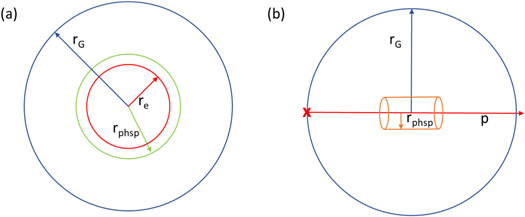
Figure 1. Schematic illustration of the cross section of the geometry set-up. (a) Source A: the electrons are generated in a 0.1 nm thick spherical shell with an outer radius of re and are emitted in random direction. The phase space file is scored on the surface of a sphere of rphsp. By varying rphsp between 1 and 100 nm, the spatial separations of the interacting tracks are in the range of less than 1 nm up to a maximum distance of around 200 nm. In the second simulation, the G-value is calculated in a sphere of rG. (b) Source B + C: the proton beam (p) is placed at one end (red cross) of the sphere in which the G-value is scored (rG = 5 μm). Protons are emitted inside the sphere towards the opposite end. The phase space file is scored at the surface of a cylinder with a length of 1 μm and a radius of rphsp= 1 μm which is placed at the center of the sphere.
Download figure:
Standard image High-resolution imageIn order to investigate the influence of inter-track interactions on both the time component, here realized by different N, and the spatial component, we set rphsp to the following different values: rphsp= 1, 10, 20, 30, 40, 50, 75, 100 nm. Since the electron density and hence the density of chemical species gets influenced by the source geometry, we expected a change of the G-value due to different rphsp. To ensure inter-track interactions, we started with the densest arrangement of electrons and then systematically decreased it. When scoring electrons at rphsp, we applied filters to the scorer so that only primary electrons with a kinetic energy of 60 eV at the scorer surface were included in the phase space file. This way, it can be avoided that the electron has already undergone interactions like ionization or excitation resulting in chemical species in the following radiolysis. These molecules would not be included in the subsequent simulation calculating the G-value. Thus, the thickness of the spherical shell was set to 0.1 nm, which is the smallest geometrical dimension that can be set in TOPAS-nBio. This way it can be avoided in advance that the particles scoring on the phase space surface already undergone inelastic interactions in this geometry component.
After the first simulation, the phase space file was modified in order to enable inter-track interaction of N = 2, 4, 5, 6, 10, 12, 15, 20, 30, 60 primary particles. These factors were chosen so that the same total number of 60 primary particles could be simulated in each simulation regardless of N. For example, choosing N = 2, chemicals produced by two different primary electrons can interact with each other. For a consistency of presentation, the reference simulations are specified as N = 1.
In the second simulation scoring the G-value, this modified phase space file was set as the particle source. The G-value was scored in a sphere with the radius of rG = 1 μm for all simulation set-ups of rphsp and N. The chosen radius ensures that all electrons and their chemicals are stopped inside this volume.
The simulations were repeated 100 times with different random seeds and final G-values were received by averaging the G-values of these 100 independent simulations.
In brief, with this simulation set-up, we studied the effect of inter-track interactions on the G-value by controlling the density of chemicals the following two ways:
- By varying rphsp, i.e. the geometrically setup, we varied the average distance between the initial electrons.
- By varying N, i.e. varying the setup on the time scale, we varied the number of tracks between which inter-track interactions can occur.
2.3.2. Particle source B + C: proton sources
In first simulations for scoring the phase space file, a proton beam with two different energies was used in separated simulations as a source: 10 MeV (source B) and 100 MeV (source C). In figure 1(b), the geometry setup is shown schematically for both proton beams. For both energies, the particle source was placed at one end of the sphere in which the G-value is scored emitting 100 primary protons inside the sphere towards the opposite end. Around each proton beam, a cylinder with an length of 1 μm and a radius of rphsp = 1 nm was positioned at the center of the sphere in order to score all secondary electrons traversing the surface of the cylinder in a phase space file. We chose this setup to reduce simulation times and still be able to investigate the difference between the high (10 MeV) and low LET (100 MeV) sources. Since the number of secondary electrons scored in one event on the cylinder surface varies with the LET, the LET-dependence can be investigated without unfeasible simulation times.
After the first simulation runs, the phase space files were modified in order to calculate inter-track interaction of the secondary electrons of N = 2, 4, 5, 10, 20, 25, 50, 100 primary protons. 5
In the following second simulations, the G-value was calculated in a sphere with radius rG = 5 μm using the modified phase space files as a particle source. This sphere size was chosen since it corresponds approximately to the size of a cell nucleus.
For statistical reasons, the simulations were performed 10 times with different random seeds 6 and final G-values were received by averaging the results of the simulations using different random seeds.
2.4. Physics and chemistry modules
In the physical stage, interactions of all primary and secondary particles with the surrounding water molecules were simulated step-by-step using the GEANT4 physics constructor G4EmDNAPhysics _option2, which is currently the default setup in TOPAS-nBio. This constructor is in detail described by Incerti et al (2018) with regard to the included physics models and was further investigated in TOPAS-nBio in our previous work (Derksen et al 2021). The following pre-chemical stage, in which the chemical species are generated, was characterized by the branching ratios and dissociation schemes, which are specified by Ramos-Méndez et al (2018) and shown in table 1. Thereby, the placement of all dissociation products is specified for each product and dissociation channel in relation to its inelastic process generating the chemicals (Bernal et al 2015). In the chemical stage, diffusion of the produced chemical species were simulated step-by-step using the Brownian motion. All chemical reactions between the molecules including their reaction rate, which were implemented in GEANT4 by Karamitros et al (2011, 2014) and extended by Ramos-Méndez et al (2018), are shown in table 2. To access these chemistry models, we used the TsEmDNAChemistryExtended module in TOPAS-nBio. In table 2, the included reactions of all eleven chemical species considered in the extended chemical list are shown. Even though oxygen is specified as a molecule in table 2, dissolved oxygen is not simulated in our simulations. The time end for chemical interactions was set to 1 μs which is the maximum value in TOPAS-nBio.
Table 1. Dissociation schemes implemented in TOPAS-nBio. Adapted from Ramos-Méndez et al 2018. © 2018 Institute of Physics and Engineering in Medicine. All rights reserved.
| Process | Probability (%) | ||
|---|---|---|---|
| Ionization state | Dissociative decay | H3O+ + OH• | 100 |
| A1B1 | Dissociative decay | OH• + H• | 65 |
| Relaxation | H2O + ΔE | 35 | |
| B1A1 | Auto-ionization |

| 55 |
| Auto-ionization | •OH+ •OH + H2 | 15 | |
| Relaxation | H2O + ΔE | 30 | |
| Rydberg, diffuse bands | Auto-ionization |

| 50 |
| Relaxation | H2O + ΔE | 50 | |
| Dissociative attachment | Dissociative decay | OH−+ •OH + H2 | 100 |
Table 2. Chemical reactions and reaction rates k considered in the chemical stage used in the module TsEmDNAChemistryExtended. H2O molecules are not listed in the reaction formulas and no product means that the reaction product is H2O. In this context,  describes an electron solvated in water. Moreover, an electron generated in the physical stage with an energy lower than the threshold of physical interactions (here 7.4 eV) is also considered as solvated. This way, its diffusion and reaction is then simulated in the chemical stage.
| No. | Reaction | k (1010/M/s) b | ||
|---|---|---|---|---|
| 1 a |

| ⟶ | 2OH− + H2 | 0.647 |
| 2 a |

| ⟶ | OH− | 2.953 |
| 3 a |

| ⟶ | OH− + H2 | 2.652 |
| 4 a |

| ⟶ | H• | 2.109 |
| 5 |

| ⟶ | OH−+ • OH | 1.405 |
| 6 a | •OH+•OH | ⟶ | H2O2 | 0.475 |
| 7 a | •OH + H• | ⟶ | No product | 1.438 |
| 8 a | H• + H• | ⟶ | H2 | 0.503 |
| 9 a | H3O + OH− | ⟶ | No product | 11.031 |
| 10 a | H2+•OH | ⟶ | H• | 0.0045 |
| 11 | •OH + H2O2 | ⟶ | HO2 | 0.0023 |
| 12 | •OH + HO2 | ⟶ | O2 | 1.0 |
| 13 |

| ⟶ | O2 + OH− | 0.9 |
| 14 | •OH + HO−2 | ⟶ | HO2 + OH− | 0.9 |
| 15 |

| ⟶ | HO−2 | 2.0 |
| 16 |

| ⟶ |

| 1.9 |
| 17 |

| ⟶ | OH− + HO−2 | 1.3 |
| 18 | H• + H2O2 | ⟶ | •OH | 0.01 |
| 19 | H• + HO2 | ⟶ | H2O2 | 2.0 |
| 20 | H• + O2 | ⟶ | HO2 | 2.0 |
| 21 a | H• + OH− | ⟶ |

| 0.002 |
| 22 |

| ⟶ | HO−2 | 2.0 |
| 23 |

| ⟶ | HO2 | 3.0 |
| 24 | H3O + HO−2 | ⟶ | H2O2 | 2.0 |
| 25 | HO2 + HO2 | ⟶ | H2O2 + O2 | 0.000076 |
| 26 |

| ⟶ | O2 + HO−2 | 0.0085 |
Notes.
a These reactions can occur directly after the pre-chemical stage. b M = 1 mol dm−3.3. Results
3.1. Particle source A: electron source
3.1.1. Radical yield at the end of the chemical phase in dependence of inter-track interactions
In figure 2, the G-value of •OH at the end of the chemical stage (t = 1 μs) is shown for all different rphsp in dependence of the number N of histories simulated simultaneously in one event using electrons with an energy of 60 eV. We chose •OH as the molecule of interest for this comparison because it is assumed that indirect DNA damages resulting from interactions of chemical species with the DNA sugar phosphate backbone are mainly caused by •OH radicals (Chapman et al 1973, Achey and Duryea 1974, Roots and Okada 1975). For all rphsp, the G-value of •OH reduces with increasing N (see figure 2). However, the magnitude of the decrease depends on rphsp. While the decrease of the G-value is approximately exponential for small rphsp, for larger rphsp (approx. rphsp ≥ 40) it is rather linear. The reason is, the smaller rphsp, the higher the density of electrons and the larger the probability of chemical reactions between molecules of different primary particles. For large rphsp, the spatial distance between primary particles is on average larger. Correspondingly, chemical species have to diffuse farther to undergo inter-track interactions. Hence, the effect of increasing N is less pronounced. Indeed, along with N, the geometry considerably effects the density of primary electrons and, consequently, the concentration of chemical radicals. This way, N and the initial, spatial distribution of the electrons affect the dynamics and complexity of the whole chemical stage significantly. Thus, we also analyzed the G-value of all six most observed molecules (H3O , H2O2 , OH− , •OH , eaq , H• , H2 ) in dependence on N in addition to •OH . Therefore, in figure 3, the G-value of these chemicals is presented as a function of N for the smallest rphsp (rphsp = 1 nm) and largest rphsp (rphsp = 100 nm) at the end of the chemical stage. For both radii, a reduction of the chemical species eaq , H3O and •OH with increasing N can be observed. In turn, the number of the species OH− , H2 and H2O2 increases with increasing N. For example, comparing the reference simulation (N = 1) and N = 60 using rphsp = 1 nm, the G-value of H2O2 is twice as high. Using rphsp = 100 nm, the amount of H2O2 increases only by around 10 % in comparison to the reference. However, for H• , no significant difference can be observed independent on the geometry and N. Furthermore, the G-value of the molecules H2O2 , •OH and OH− goes into saturation for high N, which means that further increasing N has no effect on these G-values (see figure 3). Transferring this to FLASH-RT would mean that a maximum dose rate could exits, above which an increase of the dose rate does not have an influence on the creation of chemical species in case of the inter-track interactions anymore.
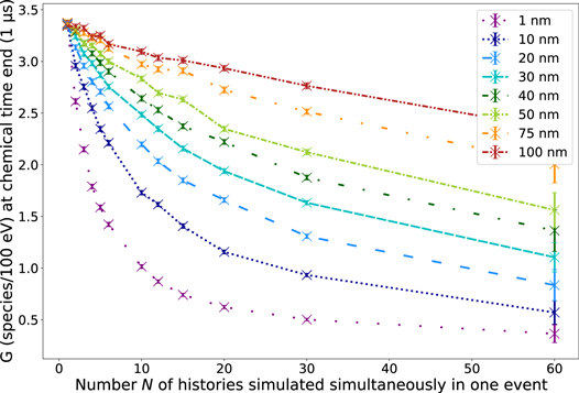
Figure 2. G-value of •OH at end of the chemical stage t = 1 μs in dependence of the number N of histories simulated simultaneously in one event for different radii rphsp between 1 and 100 nm. Data points are connected with a line for a more transparent visualization. Statistical uncertainties are represented by error bars and correspond to one standard deviation. For some data points, the symbol size is larger than the corresponding error bar.
Download figure:
Standard image High-resolution image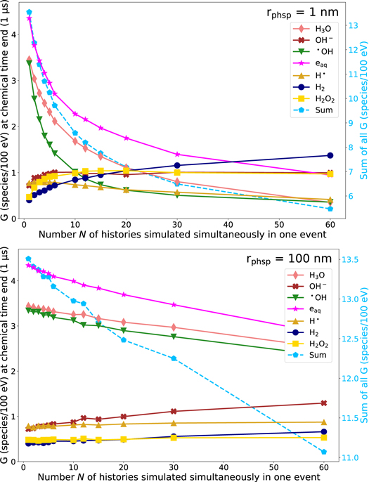
Figure 3. Left axis: G-value for different chemical species at end of the chemical stage t = 1 μs in dependence of the number N of histories simulated simultaneously in one event using rphsp = 1 nm (top) and rphsp = 100 nm (bottom). Right axis: total G-value of all molecules (dashed line). Data points are connected with a line for a more transparent visualization. The standard deviation (k = 1) is smaller than the symbol size and, hence, not depicted.
Download figure:
Standard image High-resolution imageHowever, the total G-value of all molecules decreases with increasing N. This can be explained by a significant increase of chemical reactions with an increase of N which is illustrated in figure 4 (left panel). For example, a reaction that occurs very frequently is reaction no. 6 in which H2O2 is formed from two •OH molecules (see table 2). This explains why the G-value of •OH decreases rapidly with N (see figure 3). Even though the total number of chemical species decreases with increasing N, figure 3 shows that the G-value of some molecules increase and the changes in the G-values depend on the molecule type. The reason for the different modifications of the G-value of different molecules is that some reactions occur more frequently than others with increasing N. This leads to a greater ratio of chemical reactions, that are consuming each molecule type, and reactions, that are producing each molecule type. This variable ratio in turn is responsible that the G-values of some molecules vary stronger with N than the others. The difference of the number of product and educt reactions of each chemical species is illustrated in figure 4 (right panel). Regarding the reactions of •OH exemplary, there is a negative and decreasing difference of reactions producing and consuming •OH molecules with increasing N. This means that the number of •OH molecules that are consumed in chemical reactions increases stronger with N than the number of •OH molecules that are produced in chemical reactions 7 . Hence, this results in a decrease of the G-value of •OH with N at the end of the chemical stage (see figure 3).

Figure 4. Left: total number of chemical reactions performed in the chemical stage in dependence of the number N of histories simulated simultaneously in one event using rphsp = 1 nm normalized to 100 eV of deposited energy. Diamond symbols represent the total number of all reactions and x symbols illustrate the number of the reaction •OH+•OH ⟶ H2O2 in the chemical stage. Right: Difference of the number of product molecules and educt molecules for each chemical species in the chemical stage in dependence of the number N of histories simulated simultaneously in one event using rphsp = 1 nm normalized to 100 eV of deposited energy. Counts above zero represent chemicals where the production rate is larger than the consumption rate, whereas counts smaller than zero represent chemicals where the production rate is lower than the consumption rate in the chemical stage. Statistical uncertainties are represented by error bars and correspond to one standard deviation. If the statistical uncertainty is smaller than the symbol size, no error bars are depicted.
Download figure:
Standard image High-resolution imageAll in all, the ratio of the chemical reactions consuming or producing the same chemical species is the reason why the G-value of some chemicals increases with N and for other molecules it decreases or even remains rather unchanged.
3.1.2. Time resolved radical yields
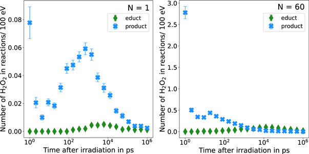
In order to validate that the diffusion ranges are responsible for the influence of the spatial separation of the primary particles, we investigated the time-dependent G-values of different rphsp, which are shown in figure 5 for •OH and H2O2 using rphsp = 1 nm and rphsp = 100 nm. In general, the amount of •OH reduces with time for all different set-ups and more H2O2 is produced towards the end of the chemical stage. For the reference simulations, this is generally in agreement with the time-evolution of the G-value calculated by Ramos-Méndez et al (2018), 8 who validated the chemistry included in TOPAS-nBio against other simulation studies and experimental data.

Figure 5. Time-dependent G-value for different number N of histories simulated simultaneously in one event. The G-values of •OH are depicted in the upper graphs using rphsp = 1 nm (left) and rphsp = 100 nm (right). The G-values of H2O2 are shown the bottom graphs using rphsp = 1 nm (left) and rphsp = 100 nm (right). Data points are connected with a line for a more transparent visualization. The time on the x-axis is scaled logarithmically. Statistical uncertainties are represented by error bars and correspond to one standard deviation.
Download figure:
Standard image High-resolution imageIn figure 5, using rphsp = 1 nm, the G-value of •OH decreases for all N with time. Already at the beginning of the chemical stage, the decrease of the G-value is more pronounced for higher N than for smaller N. The reason for this is, that for high N, the initial density of chemicals is very high and the chemicals do not need to diffuse large distances to meet a reactant. Thus, chemical reactions can already occur at the very beginning of the chemical stage (t ≤ 1 ps) explaining the differences of the G-value for different N. To quantify this, we calculated the number of reactions that occur at t ≤ 1 ps in dependence of N, which is in detail described in appendix C. All in all, the number of reactions at t ≤ 1 ps increase with N (see figure C2) explaining the differences of the G-value for different N at t = 1 ps. At the end of the chemical stage, using rphsp = 1 nm, the G-value of •OH saturates for all N. Thus, this indicates that using this setup, the G-value of •OH does not change much with time after 1 μs. For rphsp = 100 nm, the profile of the G-value of •OH is unchanged for N = 1 (see figure 5). This is because no inter-track interactions are possible and thus the density of the electrons does not matter. While for rphsp = 1 nm and N ≥ 1 variations of the G-value are already present at the beginning of the chemical stage, for rphsp = 100 nm changes due to inter-track interactions only become apparent from about 104 ps onwards. After this time period, the G-value changes for different N, which indicates that the chemicals of different primary particles diffused far enough so that inter-track interactions can occur. This can be further illustrated by calculating the theoretical mean distance between two primary particles which is approximately 1.3 nm for rphsp = 1 nm and approximately 132.3 nm, 100 times larger, for rphsp = 100 nm.
Since H2O2 is created by a reaction of two •OH molecules, the relation of the time-dependent G-values relative to N and to the different electron distributions can be explained similar to the time-dependent G-value of •OH . For rphsp = 1 nm, the G-value of H2O2 increases more strongly for higher N than for smaller N (see figure 5). For small N, the G-value is saturated at the chemical time end, whereas for N ≥ 10 the G-value decreases after about 103 ps to 104 ps. We analyzed this characteristic profile in more detail by comparing the number of reactions in which H2O2 is consumed and produced. We could show that the varying ratio between consuming and producing H2O2 reactions is responsible for the changes in the profile with increasing N. For more details, see appendix C.
For the less dense electron distribution (rphsp = 100 nm), the time-dependent G-value of H2O2 does not vary much with N similar to the G-value of •OH (see figure 5). This can be explained, as mentioned previously for •OH, by a low number of inter-track interactions due to large spatial separations of the primary tracks.
All in all, analyzing the time-dependent G-value of different rphsp, we could indicate that the variations in the G-values for different source geometries is related to the density of chemical species and the complexity of chemical reactions.
3.2. Particle source B + C: proton sources
Once the fundamental influence of inter-track interactions has been analyzed and explained using a low energy electron source, we further examined the effects of inter-track interactions of high-LET radiation sources. In figure 6, the G-value at the end of the chemical stage at t = 1 μs of different chemical species in dependence of the number N of histories simulated simultaneously in one event is shown for the 10 MeV (top) and 100 MeV (bottom) proton beam. Similar to the electron source, the total number of molecules (dashed line) decreases with increasing N for both proton sources. As before, the G-value of eaq , H3O and •OH decreases with an increasing N. In turn, the number of the species OH− , H2 and H2O2 increases with increasing N. For 100 MeV protons, the G-value of H• stays constant as it is the case for the electron source. However, for 10 MeV protons, the G-value of H• decreases slightly with increasing N. For the proton sources, saturation effects of the G-value can also be observed for high N for some molecules, such as •OH and OH− . However, using the high LET (10 MeV) proton source, these effects occur already at lower N compared to the low LET (100 MeV) source.
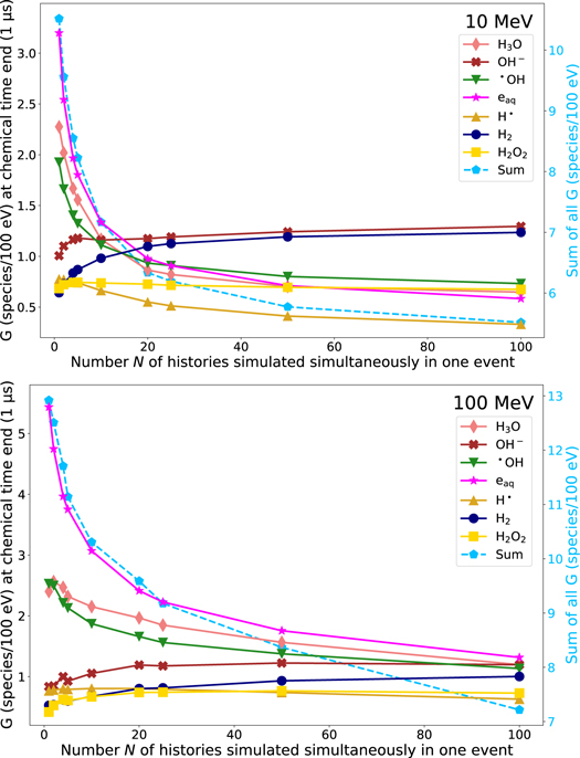
Figure 6. Left axis: G-value for different chemical species at end of the chemical stage t = 1 μs in dependence of the number N of histories simulated simultaneously in one event using a 10 MeV proton beam (top) and a 100 MeV proton beam (bottom). Right axis: total G-value of all molecules (dashed line). Data points are connected with a line for a more transparent visualization. The standard deviation (k = 1) is smaller than the symbol size and, hence, not depicted.
Download figure:
Standard image High-resolution imageWhen comparing the G-values of the proton sources without inter-track interactions (N = 1), it is obvious that the G-values of the two proton sources are already different. For example, the G-value of •OH for N = 1 using the 10 MeV source is 1.92 ± 0.01, while it is 2.53 ± 0.04 applying the 100 MeV source. This is consistent with other studies in which an LET-dependence of the G-value was observed (Burns and Sims 1981). Additionally, for the high LET source the G-value of •OH decreases in a greater extend with increasing N than the G-value of •OH using the lower LET proton source. Since the density of secondary electrons is higher in the higher LET radiation, and thus also the density of chemical species of different primary particles, here, more inter-track interactions occur in the chemical phase with increasing N, which leads to the large variation of the G-values.
4. Discussion
4.1. Discussion of the radical yield with other simulation studies and experimental studies
The variation of the G-value of eaq , •OH , H2 and H2O2 resulting from inter-track interactions (see figure 3) was also observed by Kreipl et al (2009) in a similar way simulating inter-track interactions of He2+ ions, C6+ ions and protons. Although they investigated inter-track interactions of only two primary particles in comparison to simulations without inter-track interactions, comparable to N = 1 and N = 2 in our simulations, inter-track interactions of numerous secondary particles contribute to the considerable change of the G-value. However, systematically increasing the number of inter-track interactions as done by our work group, illustrates effects of different particle and dose rates as described in section 2.2. The higher a dose rate, the more inter-track interactions can occur since an overlap of chemical tracks of different primary particles becomes more probable. Comparing this work with simulation studies that directly induced dose rates by varying the initial time of primary particles in a fixed pulse width, the same trend in the change of the G-value can be observed: Ramos-Méndez et al (2020) simulated different dose rates by simulating a constant number of primary particles delivered in pulses of different width. A maximum change in the G-value was found for a zero width pulse, which is comparable to our method in which all 60 primary particles were initialized at the same time. Even larger pulse widths of 1 ns, 1 μs and 10 μs showed significant changes in the G-value compared to conventional dose rates. Nevertheless, larger pulse widths, which are equivalent to lower dose rates, had less effects on the G-value which is in agreement with our results allowing less inter-track interactions. Comparable results were obtained by Lai et al (2021). In their simulation study, higher dose rates contributed to a smaller amount of •OH molecules. While the results of the simulation studies show a similar trend of the G-values with an increasing number of inter-track interaction or the dose rate, experimental results are not straightforward. On the one hand, Kusumoto et al (2020) observed a decrease of •OH with increasing dose rate, as investigated in the simulation studies, but on the other hand, a decrease of H2O2 with increasing dose rate was observed in some experimental trials (Montay-Gruel et al 2019, Blain et al 2022). This is in direct conflict with the results of our study and the mentioned simulation studies. Here, an increase of H2O2 has been observed for FLASH dose rates in comparison to conventional dose rates. Differences could, for example, be caused as the simulations mostly run only up to 1μs after irradiation, whereas the experimental measurements are recorded at a later point in time. In addition, dissolved molecular oxygen is not included in some of the simulations. Since •OH often forms a compound with oxygen, less H2O2 can thus be generated by •OH . However, since the amount of oxygen decreases for ultra-high dose rates, less •OH radicals might react with oxygen in comparison to low dose rates resulting in a higher production of H2O2 . For a more detailed discussion of the contrary observations of H2O2 with increasing dose rate of experimental and simulation studies we here refer to commentary by Wardman (2020).
4.2. Discussion of the radical yields in dependence of the spatial separation
As already observed when regarding the G-value of •OH for all rphsp (see figure 2), the variation of the G-value of all chemical species with N shown in figure 3 is more pronounced for rphsp = 1 nm than for rphsp = 100 nm. The influence of the spatial separation between interacting tracks was also investigated by Kreipl et al (2009) using primary He2+ ions, C6+ ions and protons. In contrast to this work, whereby the spacing of the interacting tracks is not systematically controlled but influenced by the source radius rphsp, the spatial separation in their research was systematically parameterized in the range of 0 nm and 1000 nm. Nevertheless, for all particle sources, the G-value was lowest for the smallest spatial separation of the interacting tracks as seen in our results (see figure 2). In addition, Kreipl et al observed that the number of interacting tracks had no influence on the yield of radicals for a spatial separation of 1000 nm. In comparison, in our study, the spatial separation for the largest radius (rphsp = 100 nm) cannot be larger than 200 nm, which would only be the case for N = 2 if the particles are emitted directly opposite on the sphere surface 9 . To investigate whether the saturation effect regarding the spatial separation can be reproduced with our simulations, we simulated the G-value using a radius of rphsp= 750 nm, corresponding to an approximately average spatial separation of 1000 nm of the initial electrons placed on the surface of the sphere. As shown in figure B1 in the appendix, varying N in the range of 1–100 has no influence on the G-value. Generally, the effect can be explained due to the fact that diffusion ranges of the chemical species up to 1000 nm are extremely improbable as shown by Ramos-Méndez et al (2018). Thus, chemical species of different primary particles are unlikely to react with each other at such large spatial separations. However, if N would be increased by a multiple more than 100, inter-track interactions could be triggered by the high density and thus smaller distances of the primary tracks. However, the systematic arrangement of the various primary tracks as in this study and in that of Kreipl et al (2009), do not reflect the situation of realistic extended beam fields. For particles sources with a different source geometry as well as with a different LET and hence, a corresponding different spatial arrangement of inelastic interactions, the situation of inter-track interactions might be different. However, in case of simulation time we investigated the spatial separation using electrons of low energy and not using the proton sources showing exemplary that the spatial arrangement of the source geometry has an effect on inter-track interactions. The results illustrate that the denser the primary tracks are, the more likely inter-track interactions occur reducing the amount of chemicals which is illustrated by a reduced G-value. In summary, the occurrence of inter-track interactions can be controlled by the spatial arrangement of the source geometry and by the number N of primary particles simulated simultaneously in one event, i.e. broadly the dose rate, all influencing the spatial distribution of the physical particle track.
4.3. Discussion of our approach: advantages, limitations and relevance to FLASH radiotherapy
In this study, inter-track interactions of chemicals produced by different primary particles were investigated whereas the primary particles were initialized simultaneously, that means at the same initial time. In fact, using ultra-high dose rates as in FLASH-RT, the particles are delivered at different initial times in a given pulse width as simulated for example by Ramos-Méndez et al (2020) and Lai et al (2021). However, simulating all interacting tracks simultaneously, as done in this study, actually has certain advantages: first, the impact of inter-track interactions on their own can be analyzed without other parameters affecting the results. Parameters could for example be the time structure of the pulses, the dose-per-pulse, the oxygen level and the type of the surrounding tissue cells, since these parameters obviously have an influence on the dynamics of chemical reactions. However, we first wanted to show that we are able to simulate inter-track interactions in TOPAS-nBio and investigate their influence on a first principal basis. Second, Abolfath et al (2022) pointed out that in TOPAS-nBio inter-track interactions are underestimated. By simulating all tracks simultaneously, the maximized effect of inter-track interactions can be studied.
Due to limitations in our study, a quantitative relation between N and a dose rate cannot be established. One the one hand, the temporal profile of the G-value (see figure 5) clearly illustrates that the time factor is one of the key factors for the G-value. Since in our study the particles are simulated simultaneously, that means without a separation in time, a conversion to a realistic dose rate is not feasible. One the other hand, and most importantly, the simulations are performed on microscopic scale which disables a conversion into dose, a macroscopic quantity, as discussed in detail by Abolfath et al (2020). For the purpose of calibrating the number N of particles simulated simultaneously against dose rates, the simulations will be adapted in a subsequent study. Simulations will be performed under the same conditions as experiments so that by comparing both G-values a reference to clinical dose rates can be obtained.
In this initial study regarding inter-track interactions we did not considered the role of oxygen in the simulations, which will, in turn, be taken into account in subsequent studies. Additionally, in further steps, scavengers should be included in the simulations since Ramos-Méndez et al (2021) showed that including scavengers in the chemistry simulations improves the agreement to experimental data. To improve simulations of the chemical stage and linking them to experimental conditions, the GEANT4 developers are constantly updating the code with new molecules and scavengers (Chappuis et al 2023). In addition, Wardman (2022) clarified the importance of scavenger systems since in biological tissue intracellular molecules can compete with the chemical reactions in 'pure water'. This could change the effect of inter-track interactions. But as we could show that inter-track interactions occur also in the picosecond regime, we expect that the effect of inter-track interactions is still significant in the presence of scavengers as in cellular mediums. Nevertheless, this should be investigated in further studies including the mechanisms of living cells. Until now, however, there are no established simulation codes that can cover the needs of those simulations as pointed out by Wardman (2022) and will be a quite challenging task.
Furthermore to the presented results, since we could show that inter-track interactions influence the yield of chemicals, we now apply our approach to investigate the resulting DNA damage yield in more realistic simulation set-ups e.g. including a nucleus model and optimize the spatial and temporal arrangement of initial particles.
As an outlook, TOPAS-nBio has been updated to version 2.0, which provides the simulation of inter-track interactions. Therefore, we will evaluate in a following study if comparable results can be achieved by simulations applying our approach and simulations using TOPAS-nBio 2.0.
This research showed that increasing the number of histories from which the chemical species can interact with each others, representing higher dose rates, reduces the total G-value (see figures 3 and 6) and hence more chemical reactions occur. Increasing the number N of histories simulated simultaneously in one event has a comparable effect on the G-value like increasing the dose rate as observed in an experimental study by Kusumoto et al (2020). With higher dose rates, and correspondingly more inter-track interactions, a reduction of •OH is observed. Since •OH is considered to be mainly responsible for indirect damages on the DNA, we hypothesize that this has an impact on the amount and distribution of DNA damages. This in turn, could play a crucial roll in the FLASH effect. To provide an explanation of the FLASH effect, these results are surely not sufficient enough since a difference between tumor and normal tissue response cannot be specified. But as the FLASH effect is 'the result of a multi-parameter situation' (Rothwell et al 2021), each individual variation is relevant. The exact explanation of the FLASH effect is beyond the scope of this paper but inter-track interactions may be a parameter to be considered in the mechanism.
5. Conclusion
In this work, the influence of the dose rate on the yield of chemical species was investigated by enabling inter-track interactions in radiobiological simulations using TOPAS-nBio. We developed an approach to generate inter-track interactions in the chemical stage of the simulations. It was shown that increasing the number N of histories simulated simultaneously in one event as a substitute for an increased dose rate, leads to significant changes in the yield of chemical species. In particular, the yield of •OH radicals decreases with increasing number of inter-track interactions. However, the magnitude of the variation of the chemical yields depends on the LET of the primary particles and the geometry of the source. The variation in chemical radicals may induce changes in the amount of indirect DNA damages, which in turn may be relevant in explaining the FLASH effect.
Acknowledgments
The project was supported by the Federal Ministry of Education and Research within the scope of the grant 'Physikalische Modellierung für die individualisierte Partikel-Strahlentherapie und Magnetresonanztomographie', (MiPS, Grant Number 13FH726IX6).
Data availability statement
The data cannot be made publicly available upon publication because no suitable repository exists for hosting data in this field of study. The data that support the findings of this study are available upon reasonable request from the authors.
Appendix A.: Generation of inter-track interactions in TOPAS-nBio using a phase space file.
In order to enable inter-track interactions in TOPAS, i.e. to simulate N histories in one event, we scored a phase space file of the source and modified the column called Flag to tell if this is the First Scored Particle from this History (1 means true). 10 Suppose one simulates M primary particles and scores a phase space file such that at least one particle from each primary particle reaches the surface on which the phase space file is scored. Then the mentioned column in the phase space file contains M times the flag 1. In order to simulate N histories simultaneously in one event in our simulations, the flag was modified in such a way that only every Nth entry with the flag 1 remains and the others are replaced by the flag 0. In this way, all particles between two particles with flag 1 are assigned to one event and inter-track interactions are possible.
Appendix B.: G-value using rphsp = 750 nm
For the purpose of comparing the G-value simulating a similar maximum spatial separating of interacting tracks as by Kreipl et al (2009), we performed our simulations using rphsp = 750 nm. This way, we achieved a mean spatial separation of the tracks of around 1000 nm as set by Kreipl et al. The G-values in dependence of N using rphsp = 750 nm are shown in figure B1. As observed in Kreipl et al's results, the G-value does not change with N since the distance of chemicals produced in different tracks is too large. Hence, inter-track interactions do not occur.
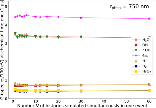
Figure B1. G-value for different chemical species at end of the chemical stage t = 1 μs in dependence of the number N of histories simulated simultaneously in one event using rphsp = 750 nm which corresponds to a mean spatial separation of the primary particles of d = 1000 nm comparable to the maximum separation set by Kreipl et al (2009). Data points are connected with a line for a more transparent visualization. The standard deviation (k=1) is smaller than the symbol size and, hence, not depicted.
Download figure:
Standard image High-resolution imageAppendix C.: Supplementary data for the analysis of the time-resolved G-value
Since we recognized that the time-dependent G-values of all N vary already at the beginning of the chemical stage at 1 ps using rphsp = 1 nm and we hypothesized, that in case of more interacting chemicals, more chemical reactions occur, we calculated the number of reactions that occur at t ≤ 1 ps in dependence of N using the electron source with rphsp = 1 nm. For this, we used the command i:Ts/ChemistryVerbosity=2 in TOPAS-nBio. This way, for each history, all chemical reactions that took place at t ≥ 1 ps are printed in the output file including the time of the reaction. For example, an extract of the output can look as illustrated in figure C1. The exemplary output in figure C1 demonstrates that chemical reactions can already take place at 1 ps which are then considered in the calculation of the G-value at 1 ps. Figure C2 shows that the number of reactions per 100 eV of deposited energy at t ≤ 1 ps increases significantly with N. Comparing N = 1 and N = 60, the number of reactions per 100 eV of deposited energy at t ≥ 1 ps increases by a factor of approximately 2. One of the reactions that occur quite frequently in this time interval is reaction no. 6 (see table 2) in which H2O2 is produced while •OH is consumed. The occurrence of this reaction increases strongly with N which explains the decreasing G-value of •OH at 1 ps with increasing N in figure 5.
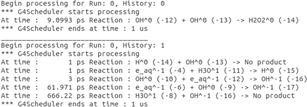
Figure C1. Exemplary extract of an output file using i:Ts/ChemistryVerbosity = 2 in TOPAS-nBio regarding all chemical reactions per history and time. The numbers in brackets behind each molecule name, correspond to the TrackIDs of the respective molecules. In this simulation, no inter-track interactions were allowed.
Download figure:
Standard image High-resolution image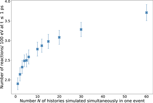
Figure C2. Mean number of chemical reactions that occurred at t ≤ 1 ps normalized to 100 eV of deposited energy. Statistical uncertainties are represented by error bars and correspond to one standard deviation.
Download figure:
Standard image High-resolution imageHowever, to be sure, that the difference of the G-value of •OH at 1 ps for different N (see figure 5) is a result of chemical reactions at t ≤ 1 ps (see figure C2) we re-calculated the G-value for t < 1 ps by considering the chemical reactions at t ≤ 1 ps. Therefore, the number of molecules that are produced through chemical reactions in this time interval are subtracted from the amount of molecules counted at 1 ps and molecules that are consumed are added to the amount of molecules counted at 1 ps. In principal, the number N of histories simulated simultaneously in one event should not have an influence on the initial yield of chemicals (here at t < 1 ps), since these are generated in the pre-chemical stage based on the physical interactions (ionization, excitation, attachment, see table 1) which do not depend on N. Hence, in principle, the initial G-value should be the same for all N, which is the case as shown in figure C3. This proves that the difference of the G-values at t = 1 ps in figure 5 is a result of chemical reactions and our approach does not affect the initial distribution of chemical radicals.
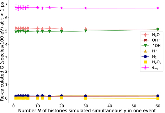
Figure C3. Recalculated, initial G-values by considering chemical reactions at t ≤ 1 ps in dependence of the number N of histories simulated simultaneously in one event. Statistical uncertainties are represented by error bars and correspond to one standard deviation (k = 1). If the statistical uncertainty is smaller than the symbol size, no error bars are depicted.
Download figure:
Standard image High-resolution imageRegarding the characteristic profile of the G-value of H2O2 using rphsp= 1 nm observed in figure 5, we examined the number of reactions in which H2O2 is involved at fixed time intervals. In figure C4, the number of H2O2 molecules included in the reactions per 100 eV of deposited energy are shown for the reference simulation without inter-track interaction (left) and for N = 60 (right). We grouped the reactions in so called educt- and product-reactions. Concretely, educt-reactions concern the reactions 5, 11 and 18 from table 2 in which H2O2 is consumed, and product-reactions include the reactions 6, 19, 24 and 25 in which H2O2 is produced. Regarding the reference simulation, the production rate of H2O2 is highest at the beginning of the chemical stage and reaches a second maximum around 1 ns. Towards the end of the chemical stage the production rate decreases. At the beginning of the chemical stage up to 103 ps, H2O2 is not consumed via educt-reactions. After this time period, educt-reactions occur in small amounts. Nevertheless, for N = 1, more H2O2 is produced than consumed during the whole chemical stage. Thus, the diminished gradient of the increasing G-value of H2O2 using rphsp= 1 nm of the reference simulation (N = 1) shown in figure 5 can be attributed to a decreased number of product-reactions and an increase of educt-reactions. In comparison, regarding the results of N = 60, the amount of H2O2 produced by chemical reactions is around 30 times larger at the beginning of the chemical stage than for the reference simulation but decreases to a greater extend with time. The number of consumed H2O2 is very low at the beginning of the chemical stage, but contrary to the reference simulation, after 103 ps, more H2O2 is consumed than produced by chemical reactions. This results in a reduced G-value of H2O2 after 103 ps for N = 60 using rphsp= 1 nm in figure 5. In conclusion, the difference between the characteristic profiles of the time-dependent G-value of the reference simulation (N = 1) and N = 60 using rphsp = 1 nm can be explained due to the fact that for the reference simulation, the production rate of H2O2 is always larger than the consumption rate, i.e. number of educt-reactions, whereas for N = 60, at the end of the chemical stage, the consumption is higher than the production of H2O2 .
Figure C4. Time-dependent evolution of the number of H2O2 molecules per 100 eV of deposited energy included in chemical reactions without inter-track interactions (left) and N = 60 (right). The reactions are grouped in educt and product reactions. In educt reactions (reaction no. 5, 11 and 18) H2O2 is consumed due to the chemical reaction, whereas in product reactions (reaction no. 6, 19, 24 and 25) H2O2 is produced. Statistical uncertainties are smaller than the symbol size and hence not depicted.
Download figure:
Standard image High-resolution image
Footnotes
- 4
The default tracking cuts for electrons are between 7.4 eV and 11 eV depending on the applied physics list (Incerti et al 2018).
- 5
Similar to the electron source, these factors were chosen so that in each simulation the same number of secondary electrons of 100 primary protons was simulated.
- 6
In contrast to the simulations using source A, 10 simulation runs showed sufficient accuracy relative to the significant increased simulation time due to the high amount of secondary electrons and the consequent increase of chemical species.
- 7
This can also be explained by the reaction rates: In sum, the reactions rates of all chemical reactions consuming •OH (reaction no. 2, 6, 7, 10–14) is 7.6728 1010/M/s whereas in sum, the reaction rates producing •OH (reaction no. 5, 18) is 1.415 1010/M/s. In general, this means that it is more likely that •OH is consumed than produced in the chemical stage.
- 8
The amount of molecules differs slightly in this study. This is due to the fact that different LETs were used and the G-value is dependent on the LET, which was shown by Ramos-Méndez et al (2018).
- 9
It should be mentioned that the spatial separation also depends on N. The larger N, the smaller the average distance of the initial tracks for the same rphsp, since the particle density becomes larger.
- 10
For details of the phase space file scorer see the TOPAS documentation https://topas.readthedocs.io/en/latest/parameters/scoring/phasespace.html.