
Abstract
Only few available interatomic interaction potentials implement the α ↔ γ phase transformation in iron by featuring a stable low-temperature bcc and high-temperature fcc lattice structure. Among these are the potentials by Meyer and Entel (1998 Phys. Rev. B 57 5140), by Müller et al (2007 J. Phys.: Condens. Matter 19 326220) and by Lee et al (2012 J. Phys.: Condens. Matter 24 225404). We study how these potentials model the phase transformation during heating and cooling; in order to help initiating the transformation, the simulation volume contains a grain boundary. For the martensitic transformation occurring on cooling an fcc structure, we additionally study two potentials that only implement a stable bcc structure of iron, by Zhou et al (2004 Phys. Rev. B 69 144113) and by Mendelev et al (2003 Philos. Mag. 83 3977). We find that not only the transition temperature depends on the potential, but that also the height of the energy barrier between fcc and bcc phase governs whether the transformation takes place at all. In addition, details of the emerging microstructure depend on the potential, such as the fcc/hcp fraction formed in the α → γ transformation, or the twinning induced in and the lattice orientation of the bcc phase in the γ → α transformation.
Export citation and abstract BibTeX RIS

Original content from this work may be used under the terms of the Creative Commons Attribution 4.0 licence. Any further distribution of this work must maintain attribution to the author(s) and the title of the work, journal citation and DOI.
1. Introduction
Molecular dynamics (MD) simulation has been used extensively in the last years to investigate the atomistic processes occurring in the α ↔ γ phase transformation in iron [1, 2]. As in all atomistic simulations, the interatomic interaction potential is decisive for the quality of the simulations. Here most often the Meyer–Entel potential [3] has been used since it predicts besides a stable bcc phase at low temperatures a transition to a high-temperature stable fcc phase. This potential thus allowed to study both the α → γ transformation and the (martensitic) γ → α transformation; it has been used to study pure iron as well as iron alloys [4–9] and the influence of various defects on the phase transformation [10–15]. The γ → α transformation corresponds to the famous martensitic transformation in iron and steel; for simplicity we will denote the reverse α → γ transformation as the austenitic transformation.
Apart from the Meyer–Entel potential, there are only two other potentials known to us that implement a high-temperature stable fcc phase in Fe; these are the potential by Lee et al (MEAM-T) [16]1—denoted by MEAM-T in his work—and the potential by Müller et al [17]. However, these do not appear to have been used for phase transformation studies up to now.
For studies of the martensitic (γ → α) transformation in iron, also potentials have been used that do not feature a high-temperature stable fcc phase, with the argument that the decay of an unstable fcc phase should be similar to that of a metastable fcc phase. Such investigations were used to study, for instance, heterogeneous nucleation, migration of the fcc–bcc phase barrier or crystallographic orientation relationships [18–27].
Recently a roadmap for computational materials science and multiscale materials modeling has been published [28] which emphasizes the importance of reliability and reproducibility in simulations. For materials simulations, an analysis of the performance and behavior of interatomic potentials for simulations is vital for the reliability of the results. In the spirit of this study, we investigate in the present paper how the α ↔ γ phase transformation in iron depends on the interatomic interaction used. To this end, we use five different potentials: Meyer–Entel potential [3], Lee et al (MEAM-T) [16], Müller et al [17], Mendelev et al [29] and Zhou et al [30]. For brevity, we will denote the potentials as the Meyer–Entel [3], Lee [16], Müller [17], Mendelev [29] and Zhou [30] potentials, respectively. Clearly, in the first three potentials both the α → γ and the γ → α transformation can be studied, while the latter two potentials only allow to model the γ → α transformation. We will present in section 3.1 several relevant properties of the potentials studied, introduce the temperature dependence of the free energies in section 3.2, and describe the dynamics of the phase transformations using MD simulation in section 3.3 and section 3.4 for the austenitic and the martensitic transformation, respectively.
2. Simulation method
We use two calculation methods: the method of metric scaling to determine the free-energy properties of Fe in the various potentials investigated; and MD simulation in order to study the dynamics of the phase transformations.
2.1. Free-energy calculations via metric scaling
We use the method of the metric scaling [31, 32] for calculating the difference in free energy, Δfbcc−fcc, between an atom in fcc and in bcc structure. This is done by transforming an fcc crystal via a linear transformation into the bcc structure along the Bain path, see below. We choose the Bain path here for its simplicity, even though it is known that several other transformation paths are relevant in the α ↔ γ phase transformation in iron and steel, such as the Nishiyama–Wassermann path [33, 34] and the Kurdjumov–Sachs path [35].
This transformation happens over 50 scaling steps. For each scaling step the change of the free-energy change is given by the work done [36, 37]:

Here the Pαα (α = x, y, z) are the stress components along the coordination axes, Aα are the perpendicular cross-sectional areas in the scaling step and dα the change of the length along the α axis to the previous scaling step.
The Bain transformation [38] contracts an fcc crystal by 21% along one ⟨100⟩ direction while expanding it by 12% along the two other ⟨100⟩ directions and thus transforms it to an equal-volume bcc crystal. The orientation relationship between the fcc and bcc crystals is

For the simulation we use cubic fcc samples with a size of (36.37 Å)3 and containing N = 4000 atoms. The x, y and z axes correspond to the ⟨100⟩ crystal directions. Since at zero pressure, the volumes of the fcc and bcc units cells are not equal, the values of the expansion and contraction have to be slightly modified to transform the fcc unit cell to a bcc unit cell, which is again at zero pressure. We illustrate the scaling process in figure 1.

Figure 1. Illustration of the three paths in transforming an fcc crystal into the bcc phase during the metric scaling process. Snapshots show the crystal after 0, 12, 25, 37 and 50 scaling steps. The colors denote the local crystal structure: green: bcc; dark blue: fcc; light blue: hcp, red: unidentified structure.
Download figure:
Standard image High-resolution imageThe simulation is performed in the NVT ensemble by controlling the temperature with the Nosé–Hoover thermostat [39, 40]. Every 50 ps a scaling step is performed so that the total transformation from the fcc crystal into the bcc crystal takes 2.5 ns. Due to thermal fluctuations, the quantities Pαα and Aβγ are averaged over 1000 data points taken during these 50 ps. The change of the free energy of the entire crystal between the original fcc structure and the structure at the scaling step i is:

where i = 0 refers to the unscaled fcc crystal and i = 50 to the completely transformed crystal in the bcc phase. For the change of the free energy for one atom we have:

where N is the number of atoms in the simulation box. For the complete Bain path the free energy is given as

and denotes the free-energy difference between fcc and bcc structure.
2.2. Molecular dynamics
For studying the dynamics of the phase transformation, we use a simulation volume with periodic boundary conditions. For the study of the bcc → fcc transition, our bcc sample has a size of 32.0 × 64.1 × 14.3 Å3 containing approximately 2500 atoms. For the martensitic fcc → bcc transformation, we use an fcc sample of size 73.3 × 146.5 × 14.3 with approximately 13 000 atoms. The bcc sample was chosen so small because otherwise—besides for the Meyer–Entel potential—no transformation would occur. It has been known for long [3] that defects help the phase transformation to nucleate; without the presence of any defects, the nucleation process may take longer than reasonable MD simulation times. We therefore include a grain boundary in the crystal; we use here a Σ5 (210) grain boundary whose influence on the transformation was studied in detail in [10]. It is a tilt grain boundary around the [001] axis, which we denote as the z direction. The x direction is the direction orthogonal to z in the GB plane, and y measures the distance perpendicular to the GB. Both crystallites are shown in figure 2. In both cases, periodic boundary conditions are applied in all Cartesian directions, such that our system actually corresponds to a multi-layered nanocrystalline material.
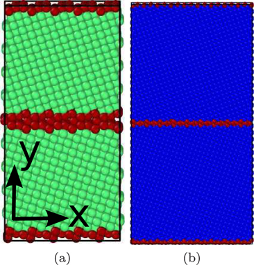
Figure 2. (a) bcc and (b) fcc samples used in the simulations. The colors denote the local crystal structure as in figure 1. The grain boundary separating the two crystalline grains is shown in red.
Download figure:
Standard image High-resolution imageThe simulation systems containing the grain boundaries are first relaxed by energy minimization using the conjugate-gradient method at 0 K and equilibrated at 10 K for 50 ps in an NPT ensemble, keeping the pressure at zero and controlling the temperature by a Nosé–Hoover thermostat [39, 40]. From this initial state, we study both the austenitic and the martensitic transformation. For the austenitic transformation, we heat the bcc sample with a heating rate of 1 K ps−1 up to 2000 K, while for the martensitic transformation, we leave the fcc sample at 10 K, since the metastable or unstable fcc phase decays at this temperature. Both these simulations are performed in an NPT ensemble at zero pressure. Temperatures above 2000 K are not relevant, since then the crystals will melt.
All calculations are performed with the open-source LAMMPS code [41]. The local lattice structure is determined by the common neighbor analysis (CNA) [42, 43]. The free software tool OVITO [44] is used for visualization of the local lattice structure.
3. Results
3.1. Potential properties
We first consider the potential properties and compare them with experimental data. In table 1, several quantities of the fcc and bcc crystals as calculated for the potentials used here—the lattice constant a, the atomic volume Ω, the cohesive energy Ecoh and the elastic constants C11, C12 and C44—are compared to experimental data. The data for the free-energy difference and the energy barrier between the phases, as well as the transformation temperature will be discussed in section 3.2 below.
Table 1. Potential properties in comparison to experimental data for bcc- and fcc-Fe. If not indicated otherwise, data are taken from the papers cited in the first row. For bcc, the elastic constants are for 4.2 K; the other experimental data are extrapolated to 0 K. For the fcc phase, the experimental values for a, Ω and Ecoh are for 295 K and the elastic constants for 1428 K. a: lattice constant, Ω: atomic volume, Ecoh: cohesive energy, C11, C12, C44: elastic constants, Tc: transformation temperature, ΔEfcc−hcp: energy difference between the fcc and the hcp phase at 0 K, ΔEbcc−fcc: energy difference between the fcc and the bcc phase at 0 K, Ebarr: energy barrier at Tc for a phase transformation from the fcc to the bcc phase.
| bcc | ||||||
|---|---|---|---|---|---|---|
| Expt. | Meyer–Entel [3] | Lee [16] | Müller [17] | Zhou [30] | Mendelev [29] | |
| a (Å) | 3.562 [48, 50] | 3.686 | 3.589 | 3.6112 | 3.6284 | 3.658 |
| Ω (Å3) | 11.298 [48, 50] | 12.520 | 11.557 | 11.773 | 11.942 | 12.237 |
| Ecoh (eV) | 4.275 [51] | 4.2407 | 4.272 | 4.2496 | 4.195 | 4.002 |
| C11 (GPa) | 154 [52] | 176.14 | 183.14 | 204.99 | 107.84 | 68.02 |
| C12 (GPa) | 122 [52] | 163.19 | 139.86 | 143.86 | 98.19 | 40.32 |
| C44 (GPa) | 77 [52] | 56.16 | 77.12 | 100.51 | 79.68 | 29.65 |
| ΔEfcc−hcp (meV) | n.a. | 3 | −8 | 4 | 1 | 2 |
| ΔEbcc−fcc (meV) | −50 [51] | −38 | −8 | −30 | −94 | −120 |
For the bcc phase, the calculated data are in good agreement with the experiment. This is not surprising since these data have been used to fit the potential. However, for the fcc phase, larger deviations are found, in particular for the elastic constants. An important issue is the atomic volume Ω, which in experiment is by 3.4 % smaller in the fcc than in the bcc phase, while it is predicted to be larger in all potentials with the exception of the Lee potential.
The energy difference between the bcc and the fcc phase at 0 K, ΔEbcc−fcc, is negative for all potentials considered here—in agreement with experiment—meaning that the bcc phase is stable at 0 K. We also include the energy difference between the fcc and the hcp phase at 0 K, ΔEfcc−hcp. Interestingly it has a positive sign for many potentials which thus predict the hcp phase to be more stable than the fcc phase at 0 K such that the order of stability is bcc < hcp < fcc. Only the Lee potential differs as it puts the energy of the fcc lattice lower than that of the hcp lattice. These findings will be relevant when discussing the relative amounts of hcp and fcc phase found in the austenitic transitions.
3.2. Free energy
The free-energy data for the potentials investigated here are assembled in figures 3–7. We start the discussion with the Meyer–Entel potential, figure 3. Figure 3(a) shows the evolution of the free energy along the Bain path. A strong temperature dependence is visible. While at low temperatures, the bcc phase is energetically more favorable, at high temperatures, the fcc phase has lower free energy. The free-energy difference between the two phases as a function of temperature is plotted in figure 3. The phase transition temperature Tc, at which both phases have equal free energy, is close to 500 K; a more exact calculation gives 487 K [49], see table 1. We also assemble in table 1 the value of the energy difference between the fcc and the bcc phase at 0 K, ΔEbcc−fcc.

Figure 3. Free energies as calculated for the Meyer–Entel potential: (a) evolution of the free energy along the Bain path for various temperatures, equation (4); (b) dependence of the free energy difference between fcc and bcc phase, equation (5), on temperature.
Download figure:
Standard image High-resolution image
Figure 4. As in figure 3, but for the Lee potential.
Download figure:
Standard image High-resolution image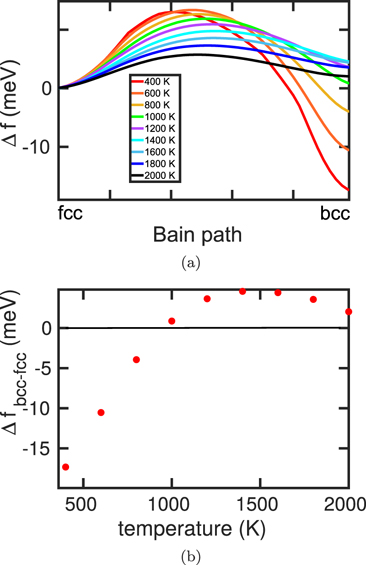
Figure 5. As in figure 3, but for the Müller potential.
Download figure:
Standard image High-resolution image
Figure 6. As in figure 3, but for the Zhou potential.
Download figure:
Standard image High-resolution image
Figure 7. As in figure 3, but for the Mendelev potential.
Download figure:
Standard image High-resolution imageA noteworthy feature of the free energy evolution along the Bain path is the occurrence of a maximum between the two phases. It denotes an energy barrier that hinders the phase transformation. Its value at the phase transition temperature, Ebarr, is 6.5 meV; here, no data from experiment or ab initio calculations appear to be available.
For the Meyer–Entel potential we see that the free-energy curve along the Bain path, figure 3(a), has a very low energy barrier at low temperatures. This is the reason why we can observe a martensitic phase transformation at low temperatures.
The Lee and Müller potentials feature the bcc–fcc transformation and their free energies are displayed in figures 4 and 5, respectively. For these two potentials, we do not show data below 400 K, since at small temperatures parts of the simulation volume on the Bain path spontaneously start phase transforming to the bcc phase. These potentials have a higher Tc than the Meyer–Entel, which is in better agreement with experiment (1184 K). Our value of Tc for the Lee potential is Tc ∼ 700 K, and thus definitely smaller than the value of Tc = 1070 K given in [16]. We presume that the use of the Gibbs–Helmholtz relation for thermodynamic integration used in [16] to determine Tc overestimates the value of Tc, as we previously observed in [32]. For the Müller potential, our value of Tc ∼ 1000 K is in good agreement with the published value of Tc = 1030 K [17].
In contrast to the Meyer–Entel potential, the Lee and Müller potentials exhibit a high energy barrier at low temperatures. This barrier will inhibit a martensitic phase transformation occurring at low temperatures. Also at the phase transition temperature, Ebarr is higher than for the Meyer–Entel potential, see table 1.
The free-energy difference, Δfbcc−fcc, has a maximum at around 1400–1500 K for both potentials. This is an indication of the tendency of Fe to return at even higher temperatures to the bcc phase. In experiment, the re-entrant bcc phase is denoted as the δ phase and it occurs at temperatures above 1665 K.
The Lee potential shows very small values of Δfbcc–fcc in a wide range of temperatures around Tc, which are less than 3 meV in the temperature range of 400–2000 K. This is in good agreement with experimental data for temperatures higher than 1000 K [51].
The Zhou and Mendelev potentials, displayed in figures 6 and 7, respectively, feature a metal that does not phase transform: the bcc phase is stable up to 2000 K. In these potentials, the cohesive energy of the bcc phase is approximately 100 meV larger than for the fcc phase, in contrast to experiment. This results in the very negative values of Δfbcc–fcc at small temperatures.
Δfbcc–fcc increases with temperature, but the fcc phase is not stabilized. Even at 2000 K, Δfbcc−fcc is around −40 ⋯ −30 meV.
3.3. Austenitic transformation
We study separately the α → γ transition, which we denote as the austenitic transformation, and the γ → α transition (martensitic transformation). In both cases we use a system including a Σ5–(210)⟨100⟩ tilt grain boundary in order to help induce the transformation.
For studying the austenitic transformation, we heat the bcc sample up from 10–2000 K with a heating rate of 1 K ps−1. We note that—in contrast to the Meyer–Entel potential—the Lee and the Müller potential did not show phase transformations for larger simulation systems. It is known [10] that the transition temperature for the austenitic transformation increases with the size of the simulation system, d, which is in our case the distance between grain boundaries. In other words, since the transformation nucleates at the grain boundaries, large distances between the grain boundaries and correspondingly small defect energy densities let the new phase nucleate only late, after substantial superheating. The higher energy barrier between fcc and bcc phase, Ebarr, table 1, prevents large systems to phase transform in the Lee and the Müller potential.
Figure 8 shows the sequence of processes occurring in the Meyer–Entel potential. The phase transformation begins with the nucleation of the new phase at the grain boundary, figure 8(a). The transformation starts at a temperature of 510 K, which is above the equilibrium transition temperature of 487 K, table 1. This is plausible, as the free-energy barrier between the fcc and bcc phase, see figure 3(a), needs some overheating to be passed.

Figure 8. Atomistic view of the phase transformation for the Meyer–Entel potential during heating a bcc crystal: (a) nucleation of the new phase and start of the transformation at 593 ps; (b) intermediate state at 594 ps; (c) the completely transformed sample at 602 ps. The colors denote the local crystal structure as in figure 1.
Download figure:
Standard image High-resolution imageAfter the nucleation of the new phase, it starts expanding over the entire sample. Figure 8(b) shows that two variants of the new phase have nucleated at the two grain boundaries bounding each grain and start coalescing. The final state at figure 8(c) shows in the upper variant a lamellar structure of mainly hcp phase including stacking fault planes, while in the lower variant fcc dominates. Between the two growing variants, a new grain boundary is established. The entire phase transformation took only 9 ps to occur.
The details of this phase transformation were already described in [10]. There a larger simulation system was used and the final phase contained only a single grain with dominant hcp fraction, in agreement with the upper variant seen in figure 8(c).
In total, we find 45.6% hcp and 37.4% fcc atoms in the transformed phase, so that in total the hcp phase is dominating. The high fraction of hcp atoms in the new phase is reasonable since we know [49] that in the Meyer–Entel potential, the energy of the hcp phase is lower than the energy of the fcc phase, see also table 1.
For the Lee potential, figure 9(a) shows that the transformation starts at a higher temperature, 969 K, in agreement with the higher transition temperature of the Lee potential, table 1. Phase detection is more inefficient at high temperatures and hence more unidentified atoms are seen in this transformation. Note that initially a high fraction of hcp atoms are produced, figure 9(b); however, they eventually tend to transfrom to a majority of fcc, figure 9(c). In the end we have 49.2% fcc and 21.5% hcp atoms. This is in agreement with the Lee potential being the only one to favor the fcc over the hcp phase, see table 1.
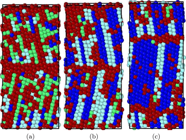
Figure 9. As in figure 8, but for the Lee potential at times of (a) 1080 ps, (b) 1081 ps, and (c) 1098 ps. The colors denote the local crystal structure as in figure 1.
Download figure:
Standard image High-resolution imageIn contrast to the Meyer–Entel potential the new phase is contained in a single grain, so that at the end of the phase transformation the system is again in a bi-crystalline structure, figure 9(c). A further analysis shows that the new grain boundary is a Σ7(451)–⟨111⟩fcc tilt grain boundary.
The phase transformation in the Müller potential, figure 10, occurs at an even higher temperature, 1054 K. Here the nucleation of the new phase occurs only on one side of the grain, figure 10(a). The new phase proceeds over the entire sample, figure 10(b), until the sample is completely transformed, figure 10(c).

Figure 10. As in figure 8, but for the Müller potential at times of (a) 1147 ps, (b) 1148 ps, and (c) 1153 ps. The colors denote the local crystal structure as in figure 1.
Download figure:
Standard image High-resolution imageThe resulting microstructure is similar to that of the upper variant in the Meyer–Entel potential, figure 8(c), and is characterized by a high hcp content: 50% of hcp and only 26% of fcc phase. This is in agreement with the high energy difference between fcc and hcp phase, ΔEfcc−hcp, see table 1, which is similar to that in the Meyer–Entel potential.
After the phase transformation, the grain boundary can be classified as a symmetrical Σ13(341)–⟨111⟩fcc—respectively a Σ39(2570)–⟨0001⟩hcp—tilt grain boundary.
We conclude that the energy barrier between fcc and bcc phase, Ebarr, table 1, determines the system size that can be used in MD simulations of the austenitic transformation. It requires small system sizes for the Lee and Müller potentials. In addition, apart from the different transformation temperatures, also the microstructures of the newly formed phases differ. This applies in particular to the fcc/hcp content of the new phase, which is correlated to the energy difference between fcc and hcp phase, ΔEfcc−hcp.
3.4. Martensitic transformation
In previous studies of the martensitic transformation using the Meyer–Entel potential [11], a cooling process was applied to an fcc crystallite in analogy to the heating process for studying the austenitic transformation. In detail, the sample was cooled from 400 K with a rate of 0.333 K ps−1; the bcc phase nucleated at 82 K, the entire transformation needed 34 ps for completion. However, when attempting to apply this scenario for the Lee or Müller potentials, the fcc phase did not transform, even when reducing the size of the simulation volume. We argue that it is the high energy barrier between fcc and bcc phase, visible in figures 4(a) and 5(a), which stay constant or even increase at small temperatures, that is responsible for impeding the transformation. Note that for the Meyer–Entel potential, this barrier decreases with temperature, figure 3(a), and hence allows the martensitic transformation to occur within a reasonable time in a MD simulation.
In the Mendelev and Zhou potentials, the fcc phase is unstable, such that it decays immediately even without a cooling process. To set all simulations of the martensitic transformation on an equal footing, we therefore set up an fcc bi-crystal containing a Σ5–(210)⟨100⟩ tilt grain boundary at 10 K, and study the transformation of this system at constant temperature. Again, for the Lee and Müller potentials, no transformation occurred within 1 ns simulation time.
For the Meyer–Entel potential, the fcc phase decays within 3.45 ps, see figure 11. The new phase nucleates in a plate structure, both at the grain boundaries and in the bulk; after growth of the plates, these coalesce and finally the bcc phase is defect-free and fills the entire grain. The grain boundary stays in place in the new bcc phase and can be described as a Σ44(774)–⟨110⟩bcc tilt grain boundary with a tilt angle of 44°. This transformation has already been described previously [11]; there, however, a larger simulation crystallite was studied, such that the final bcc phase grew in two variants, separated by twin grain boundaries.
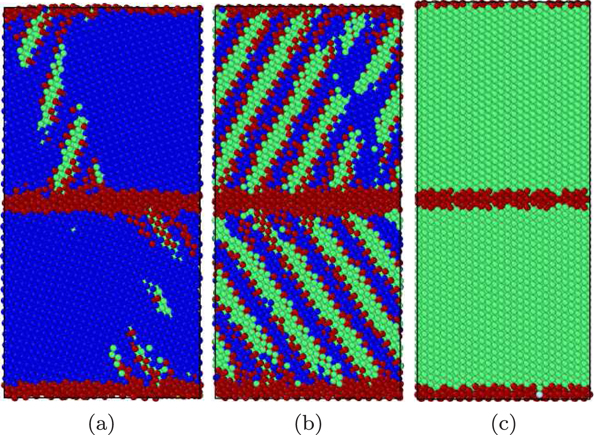
Figure 11. Atomistic view of the martensitic phase transformation for the Meyer–Entel potential during cooling an fcc crystal: (a) nucleation of the new phase and start of the transformation at 0.705 ps; (b) intermediate state at 1.55 ps; (c) the completely transformed sample at 3.45 ps. The colors denote the local crystal structure as in figure 1.
Download figure:
Standard image High-resolution imageIn the Zhou potential, figure 12, the transformation proceeds even faster, within 1.25 ps. The new phase nucleates at the grain boundary, and quickly expands throughout the entire crystal. The intermediate stage, figure 12(b), looks quite irregular with a high fraction of unidentified atoms. However, the final microstructure, figure 12(c), shows the complete transformation of the fcc phase into a rather regular array of twinned bcc variants. The original grain boundary adopts in the bcc phase the structure of a Σ9(221)–⟨110⟩bcc tilt grain boundary with a tilt angle of 38.94°.

Figure 12. As in figure 11, but for the Zhou potential at times of (a) 0.8 ps, (b) 1.05 ps, and (c) 1.25 ps. The colors denote the local crystal structure as in figure 1.
Download figure:
Standard image High-resolution imageAlso in the Mendelev potential, figure 13, the fcc phase nucleates at the grain boundaries and quickly expands into a rather irregular mixture of transformed bcc and unidentified atoms. However, the final bcc phase is defect-free and spans the entire grain in a single variant, figure 13(c). The grain boundary in the bcc phase is again a tilt boundary; it is now characterized as a Σ27(552)–⟨110⟩bcc boundary with a tilt angle of 31.59°. The entire transformation takes 2.55 ps.

Figure 13. As in figure 11, but for the Mendelev potential at times of (a) 0.625 ps, (b) 2.05 ps, and (c) 2.55 ps. The colors denote the local crystal structure as in figure 1.
Download figure:
Standard image High-resolution image
We conclude that again the energy barrier between the fcc and the bcc phase determines whether a martensitic transformation happens at all; here, now the barrier at low temperatures is relevant. For the Müller and Lee potentials the barrier is too high at low temperatures so that the metastable fcc phase does not decay at all. In contrast, for the Zhou and Mendelev potentials, there is no barrier at all; the fcc phase is unstable. The Meyer–Entel potential is intermediate, since here the barrier has a finite height at higher temperatures, but decreases toward zero at low temperatures such that at low temperatures, the martensitic transformation is possible.
While the new phase nucleates mostly from the grain boundaries—with the exception of the Meyer–Entel potential, where a small fraction of homogeneous nucleation in the bulk phase is also observed—the resulting bcc phase may have quite different microstructures, ranging from a single variant to a fine lamellar nanotwin structure for the Zhou potential. Even more astonishing is that, while the transformation starts from the same Σ5–(210)⟨100⟩ grain boundary in the fcc phase, the resulting grain boundaries in the bcc phase assume tilt angles of 31.6°, 39° and 44°.
4. Conclusions
The reliability of atomistic simulations depends on the accuracy of the interatomic interaction potential used. In the present study we investigated several interaction potentials for pure Fe in their performance on the α ↔ γ phase transformation in iron.
Certainly, the austenitic α → γ transformation can only be modeled by potentials that feature a stable high-temperature fcc phase. Only three such potentials are known, which are—besides the often used Meyer–Entel potential—the Lee and the Müller potential. Trivially, the phase transition temperature, Tc, at which fcc and bcc phase have identical free energy, differs between these potentials. But also the free-energy barrier between fcc and bcc phase, Ebarr at Tc influences the transformation, as it determines the system sizes that can be used in MD simulations; high values of Ebarr—as they show up for the Lee and the Müller potentials—require small system sizes, and render these potentials unfit for modeling the austenitic transformation in large-scale simulations.
Also the microstructure of the close-packed phase that results after the austenitic transformation depends on the potential. Here, it is in particular the fcc/hcp content of the new phase that differs among the different potentials, and which is correlated to the energy difference between fcc and hcp phase, ΔEfcc−hcp.
In the martensitic γ → α transformation, which occurs at temperatures considerably below the austenitic transformation, it is the low-temperature value of the energy barrier between fcc and bcc phase that dictates whether the transformation can occur. Here the Meyer–Entel potential features a barrier that vanishes for T → 0, such that this potential has been repeatedly and successfully been employed to study details of the martensitic transformation. On the other hand, the Lee and the Müller potentials feature barriers that stay constant or even increase with decreasing temperature. This prohibits the martensitic phase transformation to occur.
In the literature, also potentials have been employed for a study of the martensitic transformation that do not feature a stable high-temperature fcc phase; such simulations thus actually study the decay of an unstable fcc phase. There exists no energy barrier between fcc and bcc phase, Ebarr = 0. We studied the transformation occurring in two such potentials and compared to the results of the Meyer–Entel potential. We found that in all three cases, the transformation occurs at low temperatures indeed within a few ps. However, the evolving microstructure—a single bcc variant or fine nano-twinned structure—depends on the potential. In the case studied by us, the nucleation of the new phase was induced by a pre-existing grain boundary in the fcc phase; the retained grain boundaries in the bcc phase assumed widely different tilt angles between 32° and 44°, showing the influence of the potential on the forming microstructure.
While our study shows that simulation results for phase transformations such as the one studied here strongly depend on the potential employed, we emphasize the role played by the energy barrier, Ebarr, between fcc and bcc phase at the transition point. Since this barrier strongly influences the kinetics of the transition, future research should be directed on obtaining ab initio or experimental data on this quantity and to use it for potential development. At the time being, it appears that the Meyer–Entel potential has been rightly used the most in the study of the α → γ phase transformation in iron, as it allows to study the transformation for the largest systems.
Acknowledgments
We acknowledge support by the Deutsche Forschungsgemeinschaft (DFG, German Research Foundation)–project number 172116086–SFB 926. Simulations were performed at the High Performance Cluster Elwetritsch (RHRK, TU Kaiserslautern, Germany). We gratefully acknowledge conversation with Tongsik Lee about the implementation of his potential [16] in LAMMPS.
Footnotes
- 1
In the MEAM-T potential of [16], the bkgd_dyn parameter has to be set equal to 1 in LAMMPS; change Cmin(1,1,1) to 0.63 in Fe.TL.meam and repuls(1,1,1)=0.3 while attrac(1,1,1)=0.