
Abstract
In mechanical, aerospace and civil structures, cracks are important defects that can cause catastrophes if neglected. Visual inspection is currently the predominant method for crack assessment. This approach is tedious, labor-intensive, subjective and highly qualitative. An inexpensive alternative to current monitoring methods is to use a robotic system that could perform autonomous crack detection and quantification. To reach this goal, several image-based crack detection approaches have been developed; however, the crack thickness quantification, which is an essential element for a reliable structural condition assessment, has not been sufficiently investigated. In this paper, a new contact-less crack quantification methodology, based on computer vision and image processing concepts, is introduced and evaluated against a crack quantification approach which was previously developed by the authors. The proposed approach in this study utilizes depth perception to quantify crack thickness and, as opposed to most previous studies, needs no scale attachment to the region under inspection, which makes this approach ideal for incorporation with autonomous or semi-autonomous mobile inspection systems. Validation tests are performed to evaluate the performance of the proposed approach, and the results show that the new proposed approach outperforms the previously developed one.
Export citation and abstract BibTeX RIS
1. Introduction
1.1. Motivation
According to the American Society of Civil Engineers' (ASCE) report card for America's infrastructure, $2.2 trillion is needed to uplift the nation's infrastructure to 'good' condition. This budget needs to be spent over a five-year period. The current national infrastructure grade is 'D', which is close to failing [1]. There is an urgent need to develop effective approaches for the inspection and evaluation of these infrastructure systems. In addition, periodical inspections and targeted maintenance of structures will prolong their service life [2].
Despite the development of several non-destructive evaluation (NDE) techniques, visual inspection remains the predominant method currently used for the crack inspection of almost all infrastructure systems [3]. In this approach, the crack width, which provides important information about the degradation level of the component under inspection, is estimated by a trained inspector using a crack scale and a loupe. It is a subjective, tedious, time-consuming and, most importantly, highly qualitative approach. Due to these shortcomings, the need and importance of autonomous, or semi-autonomous, vision-based systems that can accurately quantify crack width have steadily increased.
The crack quantification methodology proposed in this study was developed for condition assessment of nuclear power plants. The outer layer of a nuclear power plant dome is made of concrete. This layer contains cracks that might not be due to structural deficiency (e.g., shear cracks); however, it is critical to monitor these tiny cracks to ensure that water and air cannot infiltrate into the underlying layers and cause material degradation (e.g., concrete corrosion), which leads to structural deficiencies in the long term.
In the nuclear power plant condition assessment project, the thickness threshold for crack rehabilitations was 0.25 mm (i.e., cracks thicker than 0.25 mm had to be sealed). On the other hand, due to safety constraints, the data acquisition system had to be placed 20 m away from the dome. Due to this constraint, NDE techniques that are not contact-less could not be used. Many non-contact NDE techniques had resolution issues. For instance, highly expensive laser scanners were not able to quantify cracks smaller than 1 mm from the distance of 20 m due to the large working distance. A vision-based crack detection algorithm, previously proposed by the authors, however, was capable of detecting cracks of 0.1 mm from the distance of 20 m. For this purpose, a super telephoto lens with 600 mm focal length was used. Having a system that is fully autonomous, fully contact-less, and can quantify crack thicknesses accurately and reliably, enhances the rehabilitation process, which is currently based on qualitative visual inspections, and improves the structural safety of the whole system.
Previously, the authors developed a vision-based crack detection approach that could segment the whole crack from its background [4]. In the same study, a fully contact-less crack quantification methodology was introduced. In this study, a new contact-less crack quantification approach, which can quantify crack width in unit length (e.g., a millimeter), is introduced and evaluated. The results clearly indicate that the new proposed methodology in this study is more robust than the previously developed one. In both methodologies, the 3D depth perception of the scene is used to quantify cracks. To the best of the authors' knowledge, these two methodologies are the only fully contact-less, fully autonomous crack width quantification approaches that do not need any scale attachment to the area under inspection, nor prior knowledge about the dimensions of the object under inspection. Furthermore, these methodologies are developed for field applications where several parameters, such as the camera–object distance, are uncontrollable. Here, the terminology 'cracks' is meant to refer to cracks that are dark, spatially narrow and elongated objects that have contrast with the background.
1.2. Related work
In the past twenty years, several image-based approaches have been developed for autonomous crack detection [4–24]; however, there are few studies that address the crack width quantification based on photogrammetry.
Dare et al [25] developed a crack detection methodology based on semiautomatic feature extraction, and used bilinear interpolation of pixel values to compute crack width. The measurement unit for this approach was pixels, not the unit length (e.g., a millimeter). Schutter [26] used a video microscope to monitor cracked structures. The small inspection range, and the use of a special hardware system, are among the limitations of this approach.
Ito et al [27] introduced an approach to quantify the area of fine concrete cracks. To enhance the measurement accuracy, a sub-pixel interpolation method based on the total brightness of a grayscale image was proposed. In order to estimate a crack area in millimeter squared units, a crack scale has to be attached to the surface under inspection. Yamaguchi and Hashimoto [22] improved this approach by utilizing a crack detection approach based on the percolation model and edge information. In the new approach, the crack width measurement was performed during the morphological thinning operation. This approach still requires a crack-scale attachment to estimate the crack width in millimeters. Furthermore, both of the above approaches require prior calibrations.
Benning et al [28] used photogrammetry to measure the deformations of reinforced concrete structures. A grid of circular targets is established on the testing surface. Up to three cameras capture images of the surface simultaneously. The relative distances between the centers of adjacent targets make it possible to monitor the evolution of cracks.
Sohn et al [29] developed a system to monitor crack growth. The focus of that study was to detect newly generated cracks using spatiotemporal images. The crack quantification approach was not evaluated. Furthermore, the orientation of the crack was not considered for accurate width measurement. This approach needs control targets (i.e., black–white cross marks attached on the specimen) for image registration. The experiments are conducted using a test specimen where the size of the specimen is known.
Chen et al [19] developed a semiautomatic crack measuring system using multitemporal images by utilizing the first derivative of a Gaussian filter. Quadratic curve-fitting was used to achieve sub-pixel accuracy. Their proposed system computed the crack width in millimeters in a controlled environment, assuming that the image resolution in the object space was available (i.e., the physical size of each pixel).
Chen and Hutchinson [30] developed an image-based framework for crack width quantification by computing the thickness, at each crack boundary pixel, as the shortest distance between the two edges of a given crack. In this approach, the image resolution was predetermined by controlling the image acquisition setup. To address this limitation for field applications, the use of a scale was proposed.
Lee et al [31] incorporated the thinned and boundary images of cracks to compute the crack width, at each centerline pixel, as the summation of the minimum distances between the centerline pixel and the two closest pixels on each of the crack edges. The results were promising, although this definition is not physically an accurate definition for crack width. Similarly to the current study, a pixel-to-millimeter conversion technique was used.
Zhu et al [24] developed a system to retrieve concrete crack properties, such as length, orientation and width, for automated post-earthquake structural condition assessment. These properties were reported as relative measurements related to the dimensions of the structural elements.
Jahanshahi et al [4] introduced a contact-less crack quantification approach to estimate crack thicknesses in unit length. In this approach, the orientation perpendicular to the crack centerline (i.e., thinned crack image) at each centerline pixel was defined as the crack width.
1.3. Contribution
As can be seen from the above, there are few studies regarding the vision-based quantification of crack thicknesses. Furthermore, most of the previous studies used a scale, which was attached to the region under inspection, to convert the quantified crack thicknesses from pixels to millimeters. In this study, however, a fully autonomous, fully contact-less crack quantification approach is introduced. The need for scale attachment is compensated for by developing a pixel-to-millimeter approach inspired by the human vision system that incorporates several depth parameters. In the proposed approach, a segmented crack is correlated with a set of proposed strip kernels. For each centerline pixel, the minimum computed correlation value is divided by the width of the corresponding strip kernel to compute the effective crack thickness. In order to obtain more accurate results, an algorithm is proposed to compensate for perspective errors. Validation tests are performed to evaluate the capabilities, as well as the limitations, of the proposed methodology.
1.4. Scope
Section 2 introduces the proposed approach. The detailed mathematical representation and the implementation of the proposed approach are described in sections 2.1 and 2.2, respectively. Experimental results and their discussion are presented in section 3. Section 4 includes the conclusions and future work.
2. Proposed approach
In many applications (e.g., bridge inspection), crack thickness is measured visually by an inspector. In the case of inaccessible remote regions (e.g., nuclear power plant structures), an inspector uses binoculars to detect and quantify a crack thickness. This approach is subjective and highly qualitative. In this section, a quantitative approach for estimating crack thicknesses, based on depth perception, is introduced. To quantify a crack thickness using the proposed approach, the entire crack has to be segmented from the background. In this study, an adaptive crack detection approach that can segment the whole crack from its background is used for crack extraction [4]. This crack detection approach is based on a morphological segmentation that extracts crack-like patterns. In order to further distinguish between crack-like objects and real cracks, appropriate features are computed for each segmented pattern, and a neural network classifier is used to discriminate cracks from non-crack patterns. The accuracy of the crack detection partially depends on the contrast between the crack and the background. On the other hand, the accuracy of the proposed crack quantification approach depends on how accurately and finely the crack has been segmented from the rest of the scene. Consequently, surface irregularities may cause false positives which will lead to incorrect quantifications. The reader is referred to [4] for further explanation regarding the crack detection and the issues related to false positives. Figures 1(a) and (b) show an example of a concrete crack and the segmented crack pixels, respectively. The white pixels in figure 1(b) are the extracted crack pixels.

Figure 1. An example of crack detection: (a) a concrete crack, (b) segmented crack pixels shown by white pixels.
Download figure:
Standard image2.1. Mathematical representation
Suppose Ω represents the binary image of a segmented crack. Let  be a k × k subset of Ω that centers at (u,v). We define k × k strip kernels, Γγ, that are formed by vertically arranging n orientational kernels of γ∘. γ is the angle between the orientational kernel and the horizontal direction. The correlation between
  and Γγ represents the area of the crack that is bounded between the strip edges. Consequently, the thickness orientation, θ, at (u,v) is computed as the orientation of the strip kernel which minimizes the correlation value,

where ⊙ is the correlation operator.
If n is set to be small (e.g., 11), the crack thickness does not change dramatically in the small intersection region between  and Γγ, and consequently the areas bounded by the strips are all assumed to be trapezoids for different γ values. Furthermore, the minimum correlation value corresponds to the area of the trapezoid that is approximately a rectangle. The width of this rectangle is the projection of the n-pixel length on a line which is perpendicular to the thickness orientation (i.e., the tangent at the centerline pixel). This width is ncosθ(u,v) (see figure 2). Thus, the crack thickness at (u,v) is defined as
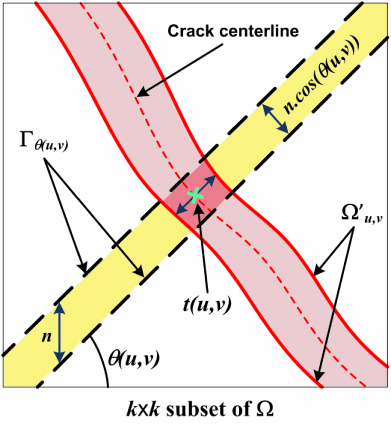
Figure 2. Graphical representation of the proposed crack thickness quantification approach.
Download figure:
Standard imageThe above approach is accurate if the camera orientation is perpendicular to the plane of the object under inspection (i.e., the region under inspection in the image is flat). In many applications, such as inspection of nuclear power plant domes, the area captured by an image can be considered as flat, without introducing too much error, since the local curvature is small (i.e., the diameter of the dome is large). Note that by using the structure from motion (SfM) problem (section 2.3), the lens distortion parameters for each camera is retrieved, and each view is undistorted prior to the quantification phase so as to improve the accuracy of the proposed approach. However, if the region of interest in the image has a significant curvature, such as a pipeline, the distorted pixels may yield poor quantification.
If the plane of the object under inspection is not perpendicular to the camera orientation (i.e., the projection surface and the object plane are not parallel), a perspective error will occur. In order to overcome the perspective error, the camera orientation vector and the normal vector of the object plane are needed. In this study, the camera orientation vector had already been retrieved using the SfM problem (section 2.3), and the normal plane could be computed by fitting a plane to the reconstructed 3D points, seen in the corresponding view, by excluding outliers using the random sample consensus (RANSAC) algorithm. In the RANSAC algorithm, a number of the 3D reconstructed points are randomly chosen and a plane is fitted to these points. Then, for each of the 3D reconstructed points, the error is defined as the distance between the point and the fitted plane. Points with errors greater than a threshold are detected as outliers. This procedure is repeated several times until the least amount of total error is computed, and the minimum number of outliers is detected.
For each centerline pixel, the numbers of pixels that are aligned with the corresponding thickness orientation are computed in the horizontal and vertical directions as follows:
and
where tx and ty are the perspective-free components of the crack thicknesses (for each centerline pixel) in the x and y directions, αx and αy are the angles between the camera orientation vector and the fitted plane's normal vector in the x and y directions (see figure 3). In other words, αx and αy are the angles between the fitted plane and the image plane in the x and y directions, respectively. The first two rows of the camera orientation matrix, retrieved from SfM, represent the x any y axes on the image plane. To compute αx, the angle between the normal vector of the fitted plane and the x axis (i.e., first row of the orientation matrix) is computed, which is the cosine inverse of the dot product of the two vectors divided by their magnitudes, and subtracted from 90°. αy is computed similarly. For each centerline pixel, the resultant of the two perspective-free components is the crack thickness,

Figure 3. Perspective error. (a) The camera orientation is perpendicular to the plane of the object (perspective error does not exist). (b) The camera orientation is not perpendicular to the plane of the object (perspective error exists). (c) 2D representation of the perspective error about the camera's 'y' axis.
Download figure:
Standard imageNote that a similar method can be used for the kernels that are formed by horizontal arrangement of the orientational kernels. In this case, the regular and perspective-free crack thicknesses are respectively
and
2.2. Implementation
In this study, the segmented crack was correlated with 35 kernels, where these kernels represented equally-incremented strips from 0° to 175°. For the 0°–45° and 135°–175° kernels, each column consisted of 11 non-zero values (see figure 4). For the 50°–130° kernels, each row consisted of 11 non-zero values. Figure 4 shows the strip kernels from 0° to 45°. The size of these kernels is 71 × 71 pixels.
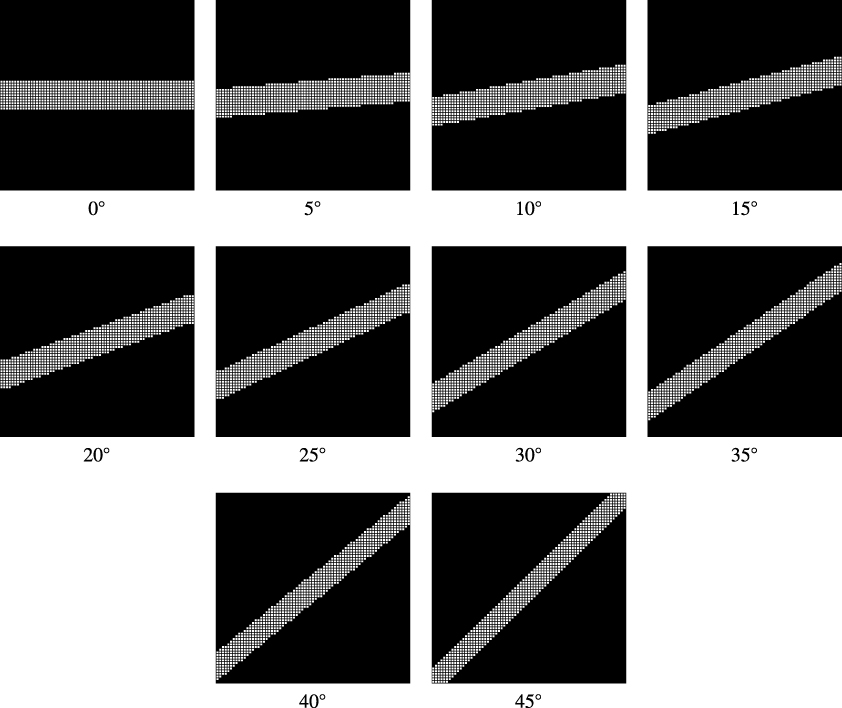
Figure 4. Strip kernels: the value underneath each kernel represents the orientation of the kernel. The black and white pixels represent zeros and ones, respectively. Each kernel is formed by vertically arranging 11 orientational kernels. Consequently, each column of these kernels consists of 11 white pixels. Other strip kernels can be built based on the kernels shown.
Download figure:
Standard imageFor each centerline pixel, obtained from morphological thinning, the strip kernel corresponding to the minimum correlation value represents the thickness orientation. Each correlation value is the area of the crack that is bounded between the strip edges. Since an 11-pixel length is relatively small, the crack thickness does not dramatically change in such a small region, and consequently the areas bounded by the strips are all assumed to be trapezoids. Furthermore, the minimum correlation value corresponds to the area of the trapezoid that is approximately a rectangle. The width of this rectangle is the projection of the 11-pixel length on a line which is perpendicular to the thickness orientation (i.e., the tangent at the centerline pixel). Finally, the crack thickness at each centerline pixel is estimated by dividing the corresponding minimum correlation value by this length. A user can interactively select a portion of a crack, and the proposed system will average the crack thicknesses for that region. This will improve the robustness of the system in the presence of noise.
Figure 5 shows an example of the proposed thickness quantification method described above. The white squares are crack pixels of a larger crack image. The blue (dark gray) and yellow (light gray) squares represent the strip kernel, centered at the red square (the dark pixel in the middle of the image), that has the minimum correlation value at the centerline pixel (red square). The kernel orientation in this example is 135°. The number of blue (dark gray) squares (i.e., 66) is the correlation value for the red centerline pixel (i.e., center pixel of this image). Consequently, the thickness for this centerline pixel is 66/(11 × cos45°) = 8.5 pixels. This thickness has to be scaled to obtain the thickness in unit length.
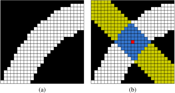
Figure 5. An example of the proposed approach for thickness quantification. (a) The white squares are crack pixels of a larger crack image. (b) The strip kernel, 135°, corresponding to the minimum correlation value for a red centerline pixel (located in the middle of the image) is shown by yellow (light gray) squares. The intersection of this strip and the crack pixels is shown by blue (dark gray) squares. The total number of intersection pixels is 66. The crack thickness at the red square is estimated as 66/(11 × cos45°) or 8.5 pixels.
Download figure:
Standard image2.3. Unit-length conversion
Using a simple pinhole camera model, the crack size represented by n pixels can be converted to unit length by the following expression:

where CS (mm) is the crack thickness represented by n pixels in an image, WD (mm) is the working distance, FL (mm) is the camera focal length, SS (mm) is the camera sensor size and SR (pixels) is the camera sensor resolution. The geometric relation between some of these parameters is shown in figure 6.

Figure 6. The geometric relation between the image acquisition parameters of a simple pinhole camera model.
Download figure:
Standard imageThe sensor size and resolution are provided by the camera manufacturer. The approximate focal length can be extracted from the image exchangeable image file format (EXIF) file. The working distance can be measured using a tape; however, in order to develop a fully contact-less system, the working distance should be obtained by using a laser range finder, a stereo vision system [32], etc. In this study, the reconstructed 3D cloud and camera locations from the SfM problem are used to estimate the working distance and the focal length. To reach this goal, first, several overlapping images of the object are captured from different views. The SfM approach aims to optimize a 3D sparse point cloud and viewing parameters simultaneously from a set of geometrically matched keypoints taken from multiple views. The SfM system developed by Snavely et al [33] is used in this study. In this system, scale-invariant feature transform (SIFT) keypoints [34] are detected in each image and then matched between all pairs of images. The RANSAC algorithm [35] is used to exclude outliers. These matches are used to recover the focal length, camera center and orientation, and radial lens distortion parameters (two parameters corresponding to a fourth-order radial distortion model [36] are estimated) for each view, as well as the 3D structure of a scene. This huge optimization process is called bundle adjustment.
To obtain the camera–object distance, a plane is fitted to the 3D points seen in the view of interest. This can be carried out by using the RANSAC algorithm to exclude the outlier points. By retrieving the equation of the fitted plane, one can find the intersection between the camera orientation line passing through the camera center and the fitted plane. The distance between this intersection point and the camera center is computed as the relative working distance. Note that the SfM problem estimates the relative 3D point coordinates and camera locations. By knowing how much the camera center has moved between just two of the views, the computed working distance can be scaled to obtain the absolute working distance.
3. Experimental results and discussion
In order to evaluate the performance of the proposed thickness quantification approach, experiments on synthetic and real cracks were carried out. Furthermore, the results from the current study were compared to the results obtained from a crack thickness quantification approach that was previously developed by the authors [4].
First, synthetic cracks were drawn by a human operator using AutoCAD®, and printed using a 600 dpi HP LaserJet printer. These crack had thicknesses of 0.4, 0.6, 0.8, 1.0, 1.2 and 1.4 mm. Six image sets were established, where each set consisted of three color images with different camera poses that were captured from the printed crack-like patterns and contained regular image noise. These eighteen images were captured by a Canon PowerShot SX20 IS with a resolution of 2592 × 1944 pixels. The crack edges were tapered in the captured images. The distance between two of the camera centers was known within each image set. For each image set, the working distances were retrieved by solving the SfM problem. The working distances in this experiment varied between 725 and 1760 mm, and were measured manually using a tape. The accurate measurement of distances between cameras has a direct relationship with the accuracy of the quantified crack thicknesses. Next, the cracks were extracted by a crack detection approach that was previously developed by the authors [4]. The proposed crack quantification was used to estimate the crack thicknesses. To increase the robustness of the proposed thickness quantification system, thicknesses within a 5 × 5 (pixels) neighborhood of each centerline were averaged. Eventually, a total of 70 721 thickness estimations were performed.
Figure 7(a) shows the mean estimated thicknesses, plotted versus the actual thicknesses. Figure 7(b) shows the corresponding standard deviation of the estimated thicknesses. The vertical axis of this graph has the same scale as the graph in figure 7(a) to facilitate the comparison between the two graphs. Figure 7(c) presents the coefficient of variation (CV) for the estimated thicknesses. As is seen from these graphs, the proposed approach in this study has closer mean estimations to the actual thicknesses with respect to the previous study, and the corresponding standard deviation values are less. Also, the coefficient of variation for the estimated thicknesses is lower for the proposed study. Thus, the proposed approach in this study performs better and more reliably.
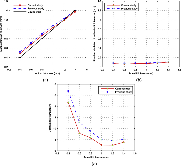
Figure 7. Estimated thicknesses versus actual thicknesses: a total of 70 721 estimations (more than 10 000 estimations for each thickness). (a) The mean estimated thicknesses, (b) the standard deviation of the estimated thicknesses and (c) the coefficient of variation of the estimated thicknesses.
Download figure:
Standard imageFigure 8 shows the histograms of the estimates presented in figure 7 for the proposed approach. The horizontal axis of each histogram is normalized by subtracting the mean and then dividing by the standard deviation. A normal histogram with the same mean and standard deviation is superposed on each histogram for comparison purposes. As is seen from this figure, the majority of the estimates are clustered around the mean measured value. Less than 0.15% of the measured values were located outside of the range shown. These values can be regarded as outliers.
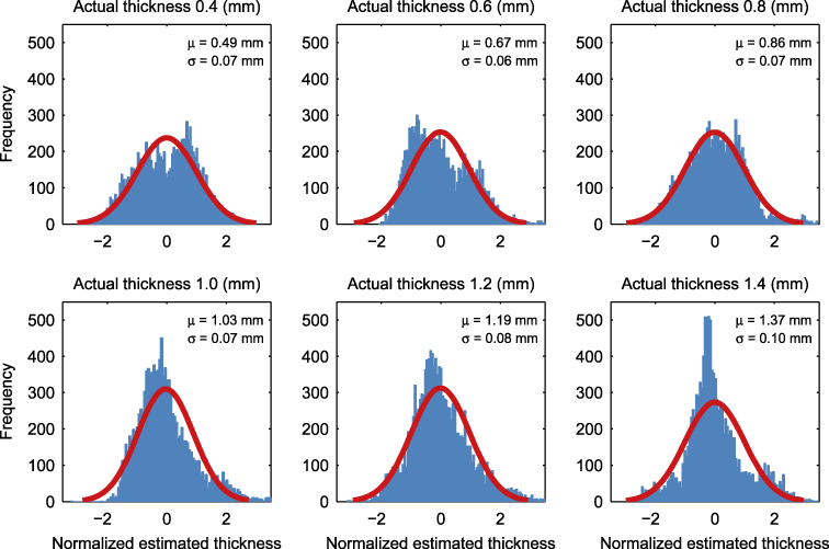
Figure 8. Histograms of the estimated thicknesses. The horizontal axis of each histogram is normalized by subtracting the mean and dividing by the standard deviation. A normal histogram with the same mean and standard deviation as the estimated values is superposed on each histogram for comparison purposes.
Download figure:
Standard imageThe mean and standard deviation of the relative errors for the estimations are shown in figures 9(a) and (b), respectively. This figure clearly shows that the proposed approach has smaller mean and standard deviation values for the relative errors compared to the previous study (i.e., the approach proposed outperforms the previous one). In these figures, as the estimated thickness increases, the mean errors fall below 10%. This is due to an increase in the number of pixels representing a given thickness (i.e., the higher the number of pixels representing a thickness, the higher the achieved accuracy). The mean error for the 0.4 mm thickness is relatively high since in some of the captured images a 0.4 mm thickness is represented by only two pixels. To address this issue, the working distance can be decreased, the focal length can be increased (zoom), the image resolution can be increased or a combination of these actions can be applied. Based on the results from figure 7, the mean error of thickness estimations for cracks that are represented by at least 6 pixels is less than 10% (i.e., crack thicknesses of 0.8 mm and greater for the proposed approach). Consequently, it is recommended to select a data acquisition system where a target thickness would be represented with a minimum of six pixels. This can be obtained by using equation (8) and setting n = 6.
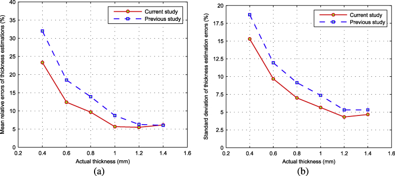
Figure 9. The relative errors of the thickness estimations: (a) the mean relative errors and (b) the standard deviation of the thickness estimation errors.
Download figure:
Standard imageThe overall mean errors shown in figure 9(a) are 10.45% and 14.24% for the current and the previous studies, respectively. This figure illustrates that the proposed approach has a smaller mean and standard deviation of the relative errors, which confirms that the this approach outperforms the previous one. Table 1 summarizes the results shown in figure 7 and 9.
Table 1. Comparison of the mean, standard deviation, coefficient of variation, mean relative error and standard deviation of the error for the current and the previous studies.
| Actual thickness (mm) | Previous study | Current study | ||||||||
|---|---|---|---|---|---|---|---|---|---|---|
| Estimation (mm) | CV (%) | Error (%) | Estimation (mm) | CV (%) | Error (%) | |||||
| Mean | Std. | Mean | Std. | Mean | Std. | Mean | Std. | |||
| 0.4 | 0.52 | 0.09 | 16.78 | 32.00 | 18.71 | 0.49 | 0.07 | 14.17 | 23.34 | 15.30 |
| 0.6 | 0.71 | 0.08 | 11.11 | 18.50 | 11.95 | 0.67 | 0.06 | 9.15 | 12.41 | 9.69 |
| 0.8 | 0.90 | 0.09 | 9.54 | 13.91 | 9.15 | 0.86 | 0.07 | 8.35 | 9.66 | 7.00 |
| 1.0 | 1.08 | 0.09 | 8.00 | 8.73 | 7.36 | 1.03 | 0.07 | 7.03 | 5.68 | 5.65 |
| 1.2 | 1.22 | 0.10 | 7.85 | 6.28 | 5.31 | 1.19 | 0.08 | 6.99 | 5.50 | 4.31 |
| 1.4 | 1.40 | 0.11 | 8.04 | 6.02 | 5.32 | 1.37 | 0.10 | 7.53 | 6.14 | 4.66 |
In order to investigate the performance of the proposed approach on real cracks, five images were taken from a concrete surface where the working distance varied from 800 to 1400 mm. The image acquisition system was identical to the one that was used in the first experiment. Twelve crack thicknesses were estimated using the proposed approach and the approach from the previous study. In order to obtain the ground truth values of the computed thicknesses, a scale (i.e., known length) was attached to the region under inspection. Next, an image was captured where the view-plane was parallel to the scene-plane. Finally, a crack thickness was quantified by converting the number of pixels representing the thickness (which was counted manually) to millimeters by using the attached scale.
Figure 10 shows the results for the computed crack thicknesses using the proposed approach and the previous approach. The results of the proposed approach are closer to the ground truth with respect to the previous approach. As is seen from this figure, the proposed approach quantifies the thickness as slightly greater than its actual thickness. This is suitable for crack monitoring applications where conservative estimations are more desirable.

Figure 10. Crack thickness quantification.
Download figure:
Standard imageTable 2 summarizes the estimated values that are plotted in figure 10. The maximum differences between the results from the current study and the previous one and the ground truth values are 0.08 mm and 0.11 mm, respectively. The relative errors obtained from the proposed approach are less than the ones obtained from the previous approach. The means of all the errors in this experiment, for the current and the previous studies, are 11.11% and 15.83%, respectively. This experiment confirms the superiority of the proposed approach; however, the computational cost of this approach is higher due to the use of larger kernels.
Table 2. Comparison of the estimated thicknesses for real cracks.
| Thickness no. | Ground truth (mm) | Previous study | Current study | ||
|---|---|---|---|---|---|
| Est. (mm) | Error (%) | Est. (mm) | Error (%) | ||
| 1 | 0.23 | 0.19 | 17.39 | 0.21 | 8.70 |
| 2 | 0.23 | 0.32 | 39.13 | 0.27 | 17.39 |
| 3 | 0.26 | 0.30 | 15.38 | 0.26 | 0.00 |
| 4 | 0.36 | 0.35 | 2.78 | 0.34 | 5.56 |
| 5 | 0.39 | 0.47 | 20.51 | 0.45 | 15.38 |
| 6 | 0.55 | 0.62 | 12.73 | 0.59 | 7.27 |
| 7 | 0.55 | 0.58 | 5.45 | 0.57 | 3.64 |
| 8 | 0.63 | 0.59 | 6.35 | 0.63 | 0.00 |
| 9 | 0.81 | 0.90 | 11.11 | 0.89 | 9.88 |
| 10 | 0.90 | 1.01 | 12.22 | 0.92 | 2.22 |
| 11 | 0.97 | 0.94 | 3.09 | 1.00 | 3.09 |
| 12 | 0.98 | 0.94 | 4.08 | 0.92 | 6.22 |
For some applications, the performance of the proposed approach may not differ dramatically from the previous approach; however, with respect to crack evolution monitoring, it has significant advantages. From an inspector's standpoint, the evolution of a crack is critical for correct diagnosis and decision making (e.g., whether a crack is problematic or not). To this end, periodical images have to be captured from an area of interest, and the images processed for accurate crack quantification. The estimated crack thicknesses at different time points have to be compared to evaluate a crack's evolution. The width of a crack may thicken at a very slow rate, making the proposed crack quantification approach of this study more desirable than the previous technique since it has a slightly better and, most importantly, more reliable performance. Furthermore, when there is a minimum allowable crack thickness on a structure (e.g., 0.25 mm crack thickness threshold for nuclear power plant domes), a more accurate and reliable quantification approach can play a critical role in categorizing the cracks.
Bundle adjustment errors, scaling errors, crack orientation errors and pixel representation errors (i.e., the number of pixels representing a thickness) are among the sources of error when quantifying a crack thickness using the above procedure. Due to some rare irregularities in an extracted crack, some parts of the thinned image might not represent the exact centerline, which causes errors too. Averaging the neighboring thickness values will help to improve the robustness of the proposed approach. The results of this study indicate that the errors are quite reasonable, and they are amenable to improvement.
4. Conclusion and future work
The predominant inspection method for civil structures is visual inspection, which is tedious, time-consuming, subjective and highly qualitative. In this approach, an inspector has to visually assess the condition of a structure. For inaccessible regions, he or she uses binoculars to detect and characterize defects. There is an urgent need to develop autonomous quantitative approaches in this field. There have been various studies regarding the detection of cracks using image processing approaches; however, there are very few studies dedicated to the quantification of crack thicknesses through photogrammetry. Furthermore, most previous studies have used a scale, which was attached to the region under inspection, to quantify the crack thicknesses in millimeters. In this study, a fully autonomous, fully contact-less crack quantification approach is introduced. In this approach, the segmented crack is correlated with a set of proposed strip kernels. For each centerline pixel, the minimum computed correlation value is divided by the width of the corresponding strip kernel to compute the effective crack thickness. In order to obtain more realistic results, an algorithm is proposed to compensate for perspective errors. Validation tests, under ambient light, were performed to evaluate the capabilities, as well as the limitations, of this methodology. The thicknesses of real concrete cracks were also quantified to illustrate the performance of the proposed approach in the presence of noise. Furthermore, the performance of the proposed approach was compared to a crack quantification approach which was developed by the authors in a previous study. The results show that although the proposed approach has higher computational cost, it outperforms the previously developed approach. Improvements in crack segmentation and centerline estimation have a direct effect on the accuracy and the robustness of the proposed approach. As part of future work, more robust centerline extraction algorithms should be developed to enhance the performance of the proposed approach.
Inaccessible regions can be assessed by using a telephoto lens. Furthermore, since the proposed approach is contact-less, its incorporation with autonomous or semi-autonomous mobile systems, such as unmanned aerial vehicles (UAV), which can move close to the structure and collect images, enables the proper inspection of inaccessible regions for cracks. As part of future work, the authors are planning to integrate the proposed methodology with commercially available microcopters to inspect inaccessible regions.
The lighting conditions (i.e., light source, orientation, density, etc) play an important role in detecting and quantifying cracks since cracks are essentially characterized based on the difference between the amount of light reflected from them and neighboring surfaces. In this study, ambient light was used; however, the use of an appropriate independent light source, which does not saturate the region under inspection, could enhance the performance and robustness of the crack detection algorithm, which would consequently improve the accuracy of the proposed quantification approach. As part of future work, the effect of lighting conditions and the use of different crack segmentation algorithms on the accuracy and performance of the proposed methodology needs to be evaluated.
Acknowledgment
This study was supported in part by grants from the US National Science Foundation.