
Abstract
Recent results on short samples of ITER-type Nb3Sn cable-in-conduit conductors have shown degradation, with the current-sharing temperature dropping slowly over several thousand current cycles. However, although such behaviour has been linked to the magnetic loads on the strands, which cause filament fracture and plastic yielding of the surrounding copper, the detailed examination of the results shows a number of inconsistencies. These suggest that the degradation may be exaggerated by artefacts of the short sample and may provide an over-conservative assessment of the in-coil performance. The behaviour of a short sample and its frictional interaction with the jacket have been analysed to consider the impact of local material modulus changes. Both an analytical approach and a finite-element simulation have been used. This paper shows that, if transverse magnetic loading causes a local reduction in the longitudinal elastic modulus of the cable in the high-field region, then the thermal compression along the cable becomes non-uniform, with a higher compression in the high field. The process develops with load cycles, due to the jacket/cable friction. If the strain change is interpreted using Jc, T, B and the strain scaling law, the predicted current-sharing temperature drop is similar to those observed during testing.
Export citation and abstract BibTeX RIS
1. Introduction
ITER magnets are typically wound from cable-in-conduit conductors made up of ∼1 mm diameter strands formed into a five-stage twisted cable inserted into a stainless-steel conduit as illustrated in the cross-sectional view in figure 1. The cables contain approximately 1000 strands and carry currents of up to 70 kA at fields up to 13 T [1, 2]. The conductors for the toroidal field (TF) and central solenoid (CS) coils rely on Nb3Sn strands which are strain-sensitive and brittle. The loading conditions on the strands are complex, consisting of the magnetic Lorentz forces directed normal to the conductor axis as well as thermal stresses directed along the axis generated by differential contraction with the jacket used to contain the cable [3]. Under some conditions, the performance of such conductors in coils has been measured to degrade as a function of load and thermal cycling [4].

Figure 1. Cross-sectional view of an ITER TF conductor (courtesy of P Lee, Florida State University).
Download figure:
Standard imageQualification and quality control tests of ITER conductors are carried out at the SULTAN facility in Switzerland [5]. SULTAN samples are about 3.6 m long, but only a small zone of the sample, of the order of 400 mm, which corresponds to the last-stage cable twist pitch, is subjected to high transverse field, while the rest only sees a low field. The conductor test conditions need to reproduce as far as possible those in a coil. However, measurements carried out on recent SULTAN TF conductor samples have shown that non-uniform strain distributions arose in the conductor jacket and evidence of strain relaxations has been observed during electromagnetic and thermal cycling that cannot be representative of conductor behaviour in a coil. This paper provides an assessment of the effects of these strain distributions on conductor performance and describes a model that could explain this behaviour. The model can then be used to select measurements on samples that can be performed to assess the extent of strain redistribution, the success of measures to eliminate it and evaluate the overall validity of a sample test.
On cycling the current in a SULTAN sample, typically we can see a steady drop in current-sharing temperature TCS, that may show stabilization after a few thousand cycles. A thermal cycle of the sample typically provokes a further drop in TCS, or, in some cases, an increase. Although this TCS degradation has been observed in coils such as the CS Insert [6], the present data show inconsistencies in the lack of stabilization, with occasional increases in TCS over a few cycles, and sometimes a crossover in the electric field versus temperature plot, with a degradation at the TCS point of 10 µV m−1 and an enhancement at electric fields of 100 µV m−1.
The experimental behaviour is limited to Nb3Sn samples and not seen in NbTi. This creates a strong suspicion that the sample behaviour is linked to the strain sensitivity of Nb3Sn and to the longitudinal strain distribution in the SULTAN samples, driven by the differential contraction between the cable and the steel jacket.
The behaviour of the superconducting cable of a SULTAN test sample and its frictional interaction with the jacket have been analysed to consider the impact of local material modulus changes in the cable. Both an analytical approach and a finite-element simulation have been used. It is shown that, if transverse magnetic loading causes a local reduction in the longitudinal elastic modulus of the cable in the high-field region, then the thermal compression along the cable becomes non-uniform, with a higher compression in the high field and lower at the ends. The process develops with load cycles, due to the friction between jacket and cable. If the strain change is interpreted using Nb3Sn superconducting performance scaling linking Jc, T, B and strain, then it is possible to predict a drop in current-sharing temperature similar to those observed.
Two mechanisms which can create a non-uniform longitudinal strain in the cable of a SULTAN sample have been identified and modelled (see also section 3.1). The first is associated with a local reduction of the effective cable modulus as a result of the application of the transverse magnetic loads (the magnetic loads cause increased strand bending which reduces the effective longitudinal stiffness of the composite cable). The second is associated with an extra local plastic deformation of the cable, also as a result of extra strand bending and copper yielding. In either case, filament fracture contributes to the reduced stiffness or plastic deformation. It is not possible to determine from this level of modelling if the increased strain in the high-field region can lead to a progressive collapse of the strands due, for example, to increased filament breakage [7] which in turn leads to further cable softening. The cable is sensitive to such effects, so that a 10% reduction of the effective cable modulus can produce a drop in cable TCS (due to a higher negative strain) of about 0.7 K.
The strain adjustment between high- and low-field regions of the cable is controlled by the frictional interaction between cable and jacket. This is likely to be variable, due to residual stresses from the jacket compaction and tolerance effects. It is likely that any disturbance in the cable (a thermal or electromagnetic cycle) will produce a gradual adjustment as slip develops along the length. However, this is inherently unpredictable.
2. SULTAN test facility
A SULTAN conductor sample (figure 2) is about 3.6 m long, with a 0.4 m high-field region of about 11 T plus about 0.75 T of self-field and two 0.8 m field gradient regions. The remaining 0.9 m has a low field (up to about 0.75 T due to the conductor self-field). The sample is made up of a pair of conductors, with joints at the bottom and at the top and is instrumented with voltage taps and temperature sensors at various locations. The measurements are carried out at fixed temperature and field and increasing current (so-called Ic runs) or at fixed current and field and increasing temperature (so-called TCS runs). The TCS runs are the most relevant to assess conductor performance. An electric field criterion of 10 µV m−1 is used to define TCS.

Figure 2. The SULTAN facility (top right, facility with test conductor in front; top left, field profile on the conductor; bottom, cross section of the background field coils). The force between the conductor pair is directed outwards on each, being reacted by supports between the conductors, with the 'underside' of the conductors being defined as the furthest surfaces of the conductors, on which the accumulated pressure acts in each, the 90° location in the diagram.
Download figure:
Standard imageFor ITER TF conductors, the SULTAN sample tests are carried out at field and current conditions which are representative of the most stringent in-coil operating conditions: the SULTAN background field is set to 10.85 T and the sample current is 68 kA. The TF conductor sample test programme calls for 1000 electromagnetic (EM) cycles followed by one warm-up/cool-down (WUCD) cycle. The EM cycles and the TCS runs are all carried out at 68 kA. The acceptance criterion is that the TCS assessed from the average of the voltage tap data at an electric field of 10 µV m−1 after 1000 EM cycles be greater than 5.8 K. The 5.8 K requirement comes from: (1) ITER TF coil design limit of 5.7 K and (2) experimental uncertainty of 0.1 K.
Extensive R&D has been performed over the last four years to give reproducible and representative results from SULTAN conductor samples. The standard ITER assembly procedure calls for: (1) low resistance (<0.5 nΩ ) solder-filled joints and (2) two sets of crimping rings at the sample ends to prevent cable/jacket slippage or longitudinal thermal strain transmitted to the joint contact surfaces (figure 3).

Figure 3. Standard SULTAN sample assembly procedure at CRPP includes two sets of 'crimping rings' at sample ends (to prevent cable/jacket slippage; courtesy of Bruzzone, CRPP).
Download figure:
Standard imageThe joints can cause current non-uniformity, which, due to the short high-field region, distorts the voltage signals and can produce an artificial impression of degradation [8]. Significant improvements in the joint resistance (to about 0.5 nΩ) and the use of multiple voltage taps have reduced the impact of current non-uniformity. It is not clear if it has been completely eliminated as some features of the sample behaviour are difficult to explain in other ways.
However, the same samples still show an 'unexpected' behaviour that does not reflect expectations based on coil measurements or on other, comparable, samples.
2.1. Load conditions in Nb3Sn conductors
The integrated thermal shrinkage coefficient of stainless steel between 933 and 4.2 K is about twice as large as that of Nb3Sn (figure 4). As a result, at the end of cool-down, in a real coil as in a 'crimped' conductor sample, the jacket is in tension along the conductor axis while the superconducting cable inside is in compression.
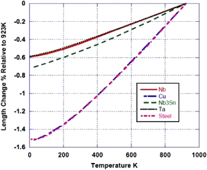
Figure 4. Integrated thermal shrinkage coefficients of various materials relevant for ITER-type cable-in-conduit conductor analyses.
Download figure:
Standard imageThe magnetic field provided by SULTAN transverse to the conductor axis creates a force on each strand also transverse to the conductor. The strand current is 76 A so the individual force on each strand is about 800 N m−1 (i.e. equivalent to 0.8 kg on each 10 m length). This load accumulates across the cable since the strands support each other. It leads to an accumulated pressure of up to about 20 MPa on the 'underside' of the cable (figure 2).
2.2. Experimental current-sharing results from SULTAN samples
The improved manufacture/instrumentation of SULTAN samples implemented in 2007/2008 enabled the successful qualification of TF conductor suppliers [2]. However, most samples have shown a steady degradation in TCS as they have undergone current cycling at peak field. Some samples have also shown a significant drop in TCS (up to 0.5 K) following a warm-up and cool-down cycle.
It is known from measurements on full size coils [4] that Nb3Sn conductors can undergo some degradation with magnetic load cycling due to the fracture of some of the superconducting filaments [7, 9]. Very high critical current strands (Jc > 1500 A mm−2) are also known to be particularly sensitive to such behaviour [10]. However, in ITER-type conductors with moderate Jc bronze and internal tin type strands, this degradation was expected to stabilize after about 1000 load cycles. Such stabilization occurred in the CS insert [6].
In some SULTAN samples, a similar stabilization is seen after about 1000 load cycles. However, in other samples, the degradation seems to continue almost linearly until at least 7000 load cycles, and is at least a factor of three larger than seen in the CS insert. Thermal cycles (to room temperature) on SULTAN samples also appear to be sometimes linked to a significant extra drop in TCS, of up to a few tenths of a degree. This only appears to occur once the sample has been exposed to magnetic load cycles.
Furthermore, over the last year a set of three nominally identical samples, have been tested in SULTAN. Each sample is made up of a leg of conductor A and a leg of conductor B. Conductors A and B were cabled and jacketed by the same suppliers, they rely on the same tubes and only differ by their strands. The two strands are bronze-process strands and their designs and morphologies are very similar. The B strand has slightly lower critical current and is more strain-sensitive than the A strand, so that the performance of B legs is expected to be slightly below that of A legs.
One convenient way to look at the SULTAN test data is to consider the effective Nb3Sn filament strain and the effective resistive transition index that can be derived by fitting the voltage data from the TCS runs using critical current density versus temperature, field and strain parametrizations, Jc (T, B and ε), that are measured in dedicated experiments for each strand type. Figure 5 shows a summary plot of effective filament strain versus EM cycle derived from the test results. Two of the B legs exhibit a large initial drop of about 0.05% between N = 1 and 50, while the other legs made with A conductors show a comparable drop upon the final WUCD. Apart from these drops, the cycling behaviour of all six conductor legs appears to be similar, with an overall EM cycling degradation of ∼0.3 K over 1000 cycles and a warm-up cool-down degradation of ∼0.1 K.
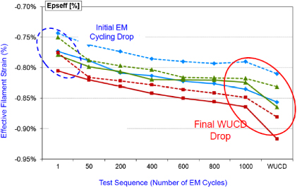
Figure 5. A set of recently tested samples, each made of one leg of A conductor (continuous line) and one leg of B conductor (dashed line) exhibited sharp performance drops either during the first 50 electromagnetic cycles (B legs) or after a final warm-up/cool-down (A legs); courtesy of A Torre, CEA.
Download figure:
Standard imageThe variation of electric field E with temperature (T) is shown in figure 6, comparing the situation at 1 EM cycle and 1000. The degradation at 10 µV m−1 is clear, but, surprisingly, the curves cross at 30 mV m−1. This sort of behaviour suggests current non-uniformity, but the cause is unknown.
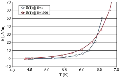
Figure 6. Inconsistent behaviour of electric field in high-field region.
Download figure:
Standard image2.3. Experimental strain measurements from SULTAN samples
The relatively thin jacket thickness of the conductor samples means that the mechanical stiffness of the jacket is not much higher than the stiffness of the cable. Changes in cable strain are therefore reflected in changes in jacket strain which can be measured by strain gauges placed on the jacket. Care is, however, required in interpreting the meaning of these strain measurements.
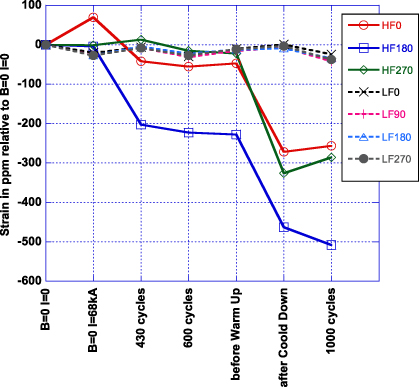
Figure 7. Strains (at zero current and zero field) measured by means of strain gauges mounted on the jacket of the B leg of one of the samples during the various phases of SULTAN testing (LFZ are low-field zone gauges, HFZ are high-field zone gauges; 90° is the underside of the cable where the magnetic forces accumulate) and 270° is the surface from which the cable pushes away. See also figure 2; courtesy of Bruzzone, CRPP.
Download figure:
Standard imageThe B leg of the last sample of the aforementioned series was equipped with strain gauges located in both the high-field and low-field zones of the jacket. The initial EM cycling and the final WUCD drops appear to be correlated with local strain relaxations in the high-field zone (HFZ) jacket section. As shown in figure 7, the LFZ strain gauges did not exhibit any change during EM cycling and WUCD, while some of the HFZ strain gauges recorded variations during the first 50 EM cycles and all of the HFZ gauges showed relaxation during the final WUCD [6]. These relaxations in the HFZ strain gauges are concomitant with the sharp TCS drops observed in figure 5.
Similar strain relaxations had already been observed in the HFZ jacket section of another SULTAN sample (TFKO2) but the amplitude of the relaxation was much smaller [11].
The existence of non-uniform strain distribution along SULTAN samples is confirmed by residual strain measurements carried out at JAEA on sample jackets after test completion [12, 13]. The residual strain is measured at room temperature by cutting successive slices of conductor.
The data for a typical sample, summarized in figure 8, consistently show that the residual strain in the HFZ of the jacket is lower than in the LFZ. The measurements in figure 8 are in reasonable agreement with those in figure 7, indicating a difference in jacket strain in the 300–500 ppm range between high field and low field that develops progressively during sample testing.

Figure 8. Summary of residual jacket strain measurements carried out at room temperature upon completion of SULTAN tests (courtesy of Y Nabara et al [13]). The HFZ is centred at 0 on the x-axis, extending ±300 mm, and the LFZ extends above 750 mm.
Download figure:
Standard imageThere are two possible interpretations for this, which may both be simultaneously applicable. Firstly, that the cable in the high-field region is softening in the longitudinal direction and/or secondly that the cable in the high-field region is slipping and relaxing its compression, leading to a higher compression in the low-field region. However, we note that the strain in the LFZ in figure 7 does not increase (as would be required by the second interpretation, although the expected increase would be small, about 50 ppm) but varies in the − 50 to 0 ppm range, suggesting that the mechanism causing the strain reduction in HFZ is, in fact, cable softening. This is supported by previous modelling work, discussed in section 3.
Such a softening means that the cable is becoming more compressed in the HFZ, by the same amount as the jacket strain relaxes. The difference between HFZ and LFZ measured at RT on the jacket is 500–600 ppm and is of the same order of magnitude as the effective filament strain change estimated from the TCS runs over the entire cold test of this sample ( − 0.06 to − 0.07% ) as shown in figure 5.
A similar difference in residual jacket strain between LFZ and HFZ was already measured at CEA in 2007 during the disassembly of the TFMC-FSJS sample after SULTAN test completion [14].
Figure 7 also suggests that the jacket strain difference develops progressively with cycling. This could be due to interaction between LFZ and HFZ as discussed in section 3, where a slip of the cable within the jacket leads to increased longitudinal compression of the HFZ by the LZF, or it could be due to continuing transverse compaction of the cable and a resultant longitudinal softening of the HFZ as the magnetic load is cycled, controlled by friction and plastic deformation of the strands locally.
3. Modelling
3.1. Background
There is an extensive background to mechanical modelling of Nb3Sn cables which, however, up to now has not been applied to the situation in SULTAN samples.
The first thorough attempt to model the strand-in-cable behaviour appears to have been in [15]. Although this analysis did not consider longitudinal variations in cable behaviour, it did address the link between longitudinal cable stiffness and the impact of the transverse magnetic loads. The analysis shows by both an analytical approach and a finite-element elasto/plastic analysis that transverse magnetic loads result in a reduction in the longitudinal elastic modulus of the cable. There are two possible mechanisms. In the first, the transverse loads create additional bending of the strands, as the cable compacts under the loads. This bending increases the longitudinal flexibility under compressive strain. In the second, the extra transverse loads on the strands create increased plastification of the copper fraction, weakening the strand stiffness in bending. Since the longitudinal stiffness of the cable depends on the strand bending stiffness, this also reduces the longitudinal modulus.
In the first case the longitudinal softening develops even though the cable remains in the fully elastic regime. By using a model for the transverse bending of the strands under magnetic loads such as developed in [16], an analytical prediction could be made of the longitudinal softening. However, the process is clearly also associated with friction between strands and plasticity of the copper component. It is not necessary to postulate that breakage of the superconducting filaments is contributing to progressive collapse of the cable, although filament fracture will increasingly develop as a result of tensile strains created by increased bending. This prediction of softening is now well supported by the strain measurements on SULTAN samples.
The subsequent modelling in this paper aims to examine the effect of this longitudinal softening in a sample where the magnetic loads are non-uniform along the length.
3.2. Analytical model
We first developed a simple mechanical model of the longitudinal sections of the cable as shown in figure 9, assuming full elastic behaviour.
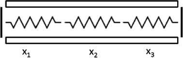
Figure 9. Diagram of the SULTAN sample. The cable is shown as three springs of different lengths in series, with x2 representing the high field and x1 and x3 the low-field lengths on each side. The cable is rigidly anchored to the jacket at the ends.
Download figure:
Standard imageThe total length of the sample is L = x1 + x2 + x3 and the differential thermal contraction between jacket and cable that arises during cool-down is △L. △L is negative (i.e. the cable would be longer than the jacket if free to move independently). To maintain compatibility between cable and jacket, a linear mechanical strain results. If the strain along the cable is distributed uniformly then it is

The elastic length changes of the three sections of cable are △L1, △L2 and △L3. In addition high-field region 2 may undergo a permanent plastic length change due to the magnetic loads of △Lp.
Therefore

The effective area of the cable is A. Let E1, E2 and E1 be the respective elastic moduli of the three cable sections 1–3 (so the high field has a different modulus). By neglecting friction between the cable and the jacket (so the whole force reaction takes place at the ends), the cable force balance gives

The increase in strain in the high field Δε2 if the strain is non-uniform is then

Putting △E2 = E2–E1 and manipulating the equations we get
For the case where △E2/E2 ≪ 1 this can be written approximately as

This enables some deductions to be made about the likely limiting behaviour of the cable strain in SULTAN samples. The model does not include friction and so represents only the final state. Since achieving this state requires frictional slip between cable and jacket, it is likely to be achieved only after load cycling and will be sensitive to the exact nature of the cable–jacket interface as regards residual compressive stresses and tolerances.
Assuming that ΔLp is zero for the moment, we note that (obviously), if x1 and x3 are small compared to x2, there is no longitudinal strain non-uniformity. This would be the ideal condition in a SULTAN sample, achieved by crimping the cable and jacket at the edges of the high field instead of at the ends of the sample. If, however, x2 is small compared to x1 + x3 (as is approximately the case with the present SULTAN sample configuration) then the strain non-uniformity is proportional to the reduction in modulus in the high-field region. The thermal strain in cables with different jacket materials has been extensively investigated in [17], including a survey of the available material database. If △E2/E2 is − 0.1 (i.e. the cable becomes softer) and εo is − 0.7% (as suggested as a likely value in [17]) then Δε2 is − 0.07%, giving a strain in the high-field region of − 0.77%.
It can also be noted that the length of the high-field region has no effect on the strain non-uniformity once x2 is a small fraction of the total length.
As will be seen at the end of the section on finite-element modelling, each 0.01% of extra compressive strain decreases the TCS of the cable by about 0.1 K. So 10% softening of the cable due to the transverse magnetic loads results in a TCS drop in the high-field region of 0.7 K. This is at least as large as the observed degradation due to filament fracture and suggests that strain non-uniformity is easily a potential source of distortion of the results obtained from SULTAN testing.
If there is a plastic deformation in the longitudinal direction in the high field that leads to a lengthening of the cable (i.e. ΔLp is positive, as would occur if the cable had a positive Poisson's ratio as a result of the transverse compression) then the increase in magnitude of the negative elastic strain is further increased. However, due to the void fraction, it seems likely that the Poisson's ratio of the cable will be close to zero. In any case, since any plastic deformation is likely also to contribute to the total strand strain, the net effect (elastic plus plastic strain) is unchanged. The plastic strain appears in the finite-element model described in section 3.3.
3.3. Finite-element model
The aim is to find a simple finite-element mesh and material representation of the cable and jacket system that allows a simulation of the potential mechanism of the degradation seen in SULTAN, including frictional effects. At this stage, we are interested in scoping calculations and can tolerate some approximation in the geometrical accuracy and physical rigour of the material model. This model will assume the cable 'softening' is due to increased plastification of the strands due to the transverse loads rather than a lower elastic modulus. The intent is to model the longitudinal friction interaction with the jacket and the extent to which sliding can be a progressive process.
For this modelling, we have chosen to use elasto-plastic material models that are already available in the ANSYS code as a standard tool for the cable to be constrained. Special-purpose material models would be better but require programming and at the moment the particular features of such models are uncertain. The features that the material model should show are:
- (1)that bending of strands under magnetic load leads to a softening or weakening of the cable in the longitudinal direction (due either to filament fracture or simply to further plasticity of the copper in the strand);
- (2)the friction between cable and jacket;
- (3)the transverse compression of the cable under the magnetic loads.
It is known from the measurement of stress–strain on reacted Nb3Sn filaments that the strands display a bilinear hardening curve [18] and that the bending of isolated strands under transverse loads is nonlinear. We do not have data to quantify how transverse and longitudinal loadings could interact but it is clear that the mechanism exists and that the plastic modulus of a strand (under axial load) can be as low as 20% of the initial elastic modulus.
We have chosen to represent the cable and jacket system using two-dimensional plane stress elements, as shown in figure 10. The elements have a thickness normal to the plane, representative of the actual cable and jacket dimensions. The top and bottom jacket elements are linked by a 2D side plate which does not contact the cable. The cable and jacket are linked at both ends (simulating the crimping rings). The cable–jacket interface is modelled by contact surface elements. The Poisson's ratio of the cable is set to 0 because the cable contains void and can be compressed in volume. The friction factor between cable and jacket is varied from 0–0.4, and 0.2 was used as the baseline value.
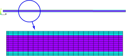
Figure 10. Sample geometry, mesh and load (sample length = 3 m, high field = 0.4 m and gradient on each side = 0.8 m). Figure 16 reflects the magnetic field profile along the sample and the magnetic forces act in a downward (negative y) direction. The lower end of the sample according to figure 2 is the left end.
Download figure:
Standard imageThere is a generic issue with the material model. With any elasto-plastic model, yielding is determined by Tresca or von Mises combined stress. In the SULTAN sample with a continuum isotropic or orthotropic model of the cable, the application of magnetic load on top of a uniaxial thermal compression from the differential contraction with the jacket results in no change or a decrease in the combined stress since the stress normal to the plane is zero. So the material model cannot be used to simulate cable weakening in the high-field region. A special material model could be developed that links transverse pressure to longitudinal modulus. However, there is a simpler approach for these calculations: artificially putting the cable in tension by simulating that, during cool-down, the cable shrinks longitudinally relative to the jacket instead of expanding. In this case, the application of magnetic pressure creates a higher Tresca stress and local yielding can be modelled.
It has to be emphasized that this reversal of strain direction does not affect the validity of the analysis but is an artefact to utilize an existing material model. It means that longitudinal x-direction stresses need to be interpreted as negative, as do the x-direction strain and slip directions. Since the Poisson's ratio is zero, the x-tension/compression is decoupled from the y direction.
Load conditions are applied as follows.
- (1)Longitudinal thermal strain of 0.7% applied between cable and jacket; minor transverse shrinkage (to stabilize model) since the cable is largely copper in the transverse direction. This simulates the cool-down of the steel-Nb3Sn system from the reaction heat treatment (about 650 °C).
- (2)
- (3)Warm-up and cool-down. The thermal strain between cable and jacket due to a warm-up to room temperature is 0.12%, so that the 4 K thermal strain of 0.7% is reduced to 0.58% and then reapplied.
The loads are applied in the following sequence:
- (a)(1) is applied;
- (b)200 applications of (2);
- (c)one application of (3);
- (d)100 applications of (2).
The elasto-plastic model is shown in figure 11. We use an initial elastic modulus of 50 GPa, followed by a plastic modulus in the range of 2.5–20 GPa, 2.5 GPa being used as the baseline. The yield stress is 100 MPa (0.2% strain) so that, after the first cool-down, the cable is in the fully yielded condition. The transverse modulus is 2 GPa and is fully elastic.

Figure 11. Longitudinal material model (elasto-plastic bilinear kinematic hardening) with plastic modulus = 2.5 GPA. Transverse E = 2 GPa.
Download figure:
Standard imageIn terms of yielding, this model implies that the extra strain in the high-field region is caused by a plastic deformation (the term △Lp in the analytical model of section 3.2). The bilinear hardening model does not create a cable with a reduced modulus, but a cable that work-hardens with load cycles. The yield envelope is determined by a Tresca stress of 100 MPa. In the transverse direction the modulus is unaffected by yield and the response remains elastic. In the longitudinal direction, the addition of the magnetic loads creates a plastic yielding. Expressed in terms of compressive strain (rather than the tension used in the finite-element model) the cable gets shorter (△Lp is negative) and the extra strain in the high-field region is △Lp/x2. This develops slowly since the cable yielding is controlled by the lengths 1 and 3 on each side, which need to slip against the jacket for yielding to occur.
3.4. Finite-element analysis results
The results of the analysis are presented in figures 12–26 and are largely self-explanatory.

Figure 12. Longitudinal stress on first magnetic load cycle MPa (read as compressive).
Download figure:
Standard image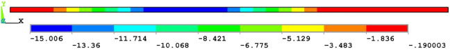
Figure 13. Transverse stress (due to magnetic load) on first magnetic load cycle (MPa).
Download figure:
Standard image
Figure 14. Tresca stress MPa on first magnetic load cycle.
Download figure:
Standard image
Figure 15. Longitudinal thermal strain during application of first load cycle (read as compressive).
Download figure:
Standard image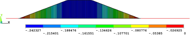
Figure 16. Contact gap, millimetre, between cable and jacket during application of first load step.
Download figure:
Standard image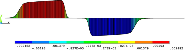
Figure 17. Relative sliding of contact elements (on the cable side towards which the pressure acts). In the model, positive sliding is in the − ve x direction (so that sliding increases the tension of the high-field cable region of the sample). This increase in cable tension has then to be read as negative for the purposes of interpretation of the superconducting behaviour.
Download figure:
Standard image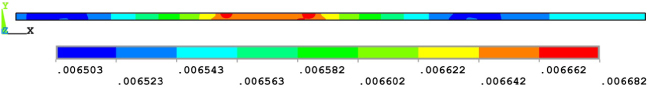
Figure 18. Longitudinal thermal strain after application of first load cycle (read as compressive).
Download figure:
Standard image
Figure 19. Relative sliding of contact elements (on the cable side towards which the pressure acts).
Download figure:
Standard image
Figure 20. Relative sliding of contact elements (on the cable side towards which the pressure acts).
Download figure:
Standard image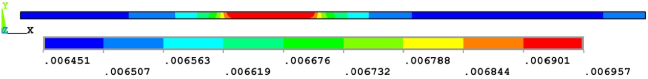
Figure 21. Longitudinal thermal strain after application of 200 load cycles (read as compressive).
Download figure:
Standard image
Figure 22. Longitudinal thermal strain after application of 200 load cycles and a warm-up/cool-down cycle (read as compressive).
Download figure:
Standard image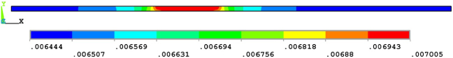
Figure 23. Longitudinal thermal strain after application of 200 load cycles, a warm-up/cool-down cycle and one further load cycle (read as compressive).
Download figure:
Standard image
Figure 24. Longitudinal thermal strain after application of 200 load cycles, a warm-up/cool-down cycle and 100 further load cycles (read as compressive).
Download figure:
Standard image
Figure 25. Relative sliding of contact elements after application of 200 load cycles, a warm-up/cool-down cycle and 100 further load cycles (on the cable side towards which the pressure acts).
Download figure:
Standard image
Figure 26. Longitudinal thermal strain after application of 200 load cycles and warm-up (read as compressive), at room temperature.
Download figure:
Standard imageThe thermal longitudinal strain after the first cool-down is 0.006 56 (0.656%). The application of the first magnetic load cycle changes the longitudinal strain (figure 12) due to plastic yielding and a subsequent strain adjustment. The transverse stress (figure 13) reflects the magnetic loads, with a peak pressure of about 15 MPa in the cable.
The contact gap between cable and jacket (figure 16) is about 0.24 mm, which corresponds to estimates from the model coil programme. The pattern reflects the magnetic loads accurately. Relative sliding in the longitudinal direction is about 0.002 mm and is symmetric in the high-field region. The sliding is low since it is prevented by the magnetic pressure acting on one surface.
Following removal of the transverse load, a non-uniform longitudinal strain system is created, as shown in figure 18 (compare with thermal longitudinal strain of 0.656% after the first cool-down), with a reduction in strain magnitude at the ends and an increase in the high-field region. The relative sliding of the jacket–cable interface increases to 0.03 mm (so removing the transverse load allows relative slip to occur). After 200 cycles, the relative slip increases to 0.11 mm (see figure 20) and the total longitudinal strain magnitude in the high-field region further increases to match.
The warm-up/cool-down cycle causes the strain magnitude to further increase (figure 22) and the next load cycle (figure 23) increases it again. Figure 24 shows the longitudinal strain after a further 100 load cycles and figure 25 shows the relative slip (now 0.15 mm).
Figure 26 shows the thermal strain in the cable after the first 200 load cycles and after warm-up to room temperature.
Figure 27 summarizes the overall changes in longitudinal strain according to the number of load cycles. We have also transformed these strain changes into an equivalent drop in sample TCS using the ITER Nb3Sn strand scaling [19] and assuming an initial sample TCS of 6.1 K. The first 200 load cycles produced a drop in TCS of about 0.4 K, and the warm-up/cool-down cycle, a further drop of about 0.05 K.
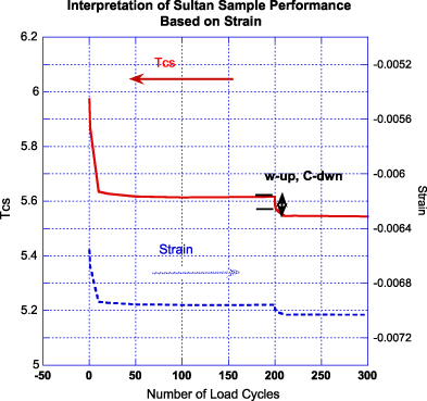
Figure 27. Interpretation of the peak strain in the high-field region (without load) as a loss of TCS.
Download figure:
Standard image4. Conclusions
Two mechanisms that could create a non-uniform longitudinal strain in the cable of a SULTAN sample have been identified and modelled. The first is associated with a local reduction of the effective cable modulus as a result of the application of the transverse magnetic loads (the magnetic loads cause increased copper strand bending and yielding, thus reducing the effective longitudinal stiffness of the composite cable). The second is associated with an extra local plastic deformation of the cable, also as a result of extra strand bending and copper yielding. In either case, filament fracture could be contributing to the reduced stiffness or plastic deformation. At this level of modelling it is not possible to determine if the increased strain in the high-field region can lead to a progressive collapse of the strands due, for example, to increased filament breakage which in turn leads to further cable softening.
The cable is sensitive to such effects, so that a 10% reduction of the effective cable modulus can produce a drop in cable TCS (due to a higher negative strain) of about 0.7 K.
The strain adjustment between high- and low-field regions of the cable is controlled by the frictional interaction between cable and jacket. This is likely to be unpredictable and variable, due to residual stresses from the jacket compaction and tolerance effects. It is likely that any disturbance in the cable (a thermal or magnetic cycle) will produce a gradual adjustment as slip develops along the length.
Although the finite-element model that has been developed is not fully representative of the likely mechanical degradation of an Nb3Sn cable with load cycling, it is adequate to show how a local plastic deformation can provide a mechanism for friction-controlled compressive strain redistribution inside a straight conductor sample with a very local short high-field region inside a steel jacket. The cable strain readjustment in the finite-element model is substantially complete after ten load cycles but the model includes only plastic deformations, not elastic softening. The model shows how a warm-up and cool-down cycle produces a further strain redistribution and a further drop in TCS in the high-field region.
The relative adjustment of the cable inside the jacket is very small (<0.2 mm) and will be difficult to detect by visual inspection of a sample after testing. The very small movements which can produce such a drop in TCS also mean it will be quite difficult to design samples which avoid such effects. Crimping the jacket close to the high-field region would be adequate, but the crimps need to be quite deeply embedded into the cable.
By comparing the predictions of strain in the high-field region of the sample to the strand critical current through the Nb3Sn B–T strain parametrization, the model can be used to predict the drop in TCS likely to be observed. This matches the order of the experimental observations (about 1 K).
The model also provides predictions that could be useful to confirm if the effect is actually occurring.
- (1)The degradation observed with cycling is not necessarily a progressive damage of the Nb3Sn strands but could be a localized ratcheting of the compressive strain from the conductor jacket. Therefore, strand samples taken from the high-field region of a conductor with ratcheting and a very low final TCS should not be more degraded than those taken from a conductor that does not degrade.
- (2)There is a non-uniform strain distribution along the cable after a final warm-up (figure 19) that could possibly be detected by neutron diffraction measurements performed on an intact conductor sample. However, the cable is a complex system of strain values in individual strands and it may be difficult to detect an average trend along the length.
- (3)Degradation with magnetic and/or thermal cycling should eventually stabilize if it is caused by softening and not by progressive filament fracture.
If the mechanism identified by the model is correct, then such 'degradation' observed in SULTAN samples is not necessarily all degradation and will not occur to the same extent in coils. The drop in TCS is due to increased axial compressive strain in the high-field region, not necessarily filament fracture. It arises because in a straight sample the engagement of the cable with the jacket is weak and, once disengaged, the cable can move. In a coil the conductor is curved and there are no such localized regions of high field.
The views and opinions expressed herein do not necessarily reflect those of the ITER Organization.