


ABSTRACT
We investigate the directional distribution of heavy neutral atoms in the heliosphere by using heavy neutral maps generated with the IBEX-Lo instrument over three years from 2009 to 2011. The interstellar neutral (ISN) O&Ne gas flow was found in the first-year heavy neutral map at 601 keV and its flow direction and temperature were studied. However, due to the low counting statistics, researchers have not treated the full sky maps in detail. The main goal of this study is to evaluate the statistical significance of each pixel in the heavy neutral maps to get a better understanding of the directional distribution of heavy neutral atoms in the heliosphere. Here, we examine three statistical analysis methods: the signal-to-noise filter, the confidence limit method, and the cluster analysis method. These methods allow us to exclude background from areas where the heavy neutral signal is statistically significant. These methods also allow the consistent detection of heavy neutral atom structures. The main emission feature expands toward lower longitude and higher latitude from the observational peak of the ISN O&Ne gas flow. We call this emission the extended tail. It may be an imprint of the secondary oxygen atoms generated by charge exchange between ISN hydrogen atoms and oxygen ions in the outer heliosheath.
Export citation and abstract BibTeX RIS
1. INTRODUCTION
The Interstellar Boundary EXplorer (IBEX) is a small explorer mission, which is designed to measure neutral atoms across the entire heliosphere and the heliospheric interfaces (McComas et al. 2009a). The IBEX observations provide maps of the globally distributed neutral atom fluxes. The maps obtained with the IBEX cameras at energies ≥0.1 keV reveal an unpredicted "Ribbon" of enhanced neutral atom emissions, which has approximately two to three times higher flux than the surrounding regions and appears to be ordered by the external magnetic field in the very local interstellar medium (McComas et al. 2009b; Schwadron et al. 2009). The IBEX observations show that the Ribbon appears in the energy range from 0.1 to 6 keV with a maximum contrast at solar wind energies around 1 keV (Fuselier et al. 2012; Galli et al. 2014; McComas et al. 2014; Schwadron et al. 2014).
In addition to heliospheric neutral atoms, the IBEX-Lo sensor, which covers the energy range from 0.01 to 2 keV, directly observes the interstellar atoms penetrating into the inner heliosphere due to the motion of the heliosphere relative to the local interstellar medium (Möbius et al. 2009, 2012). This incoming neutral gas of the local interstellar medium is deflected by solar gravity and depleted by ionization. The IBEX-Lo observations provide the first direct observations of interstellar neutral (ISN) H and O&Ne atoms (Möbius et al. 2009) and the only direct observations of interstellar He other than the prior Ulysses measurements (Witte 2004). The maps of neutral H and He atoms have been used to determine physical parameters of the ISN He gas flow (Bzowski et al. 2012; Möbius et al. 2012; Kubiak et al. 2014) and the energetic, spatial, and temporal distribution of energetic neutral atoms from the heliosheath (Fuselier et al. 2012, 2014; Galli et al. 2014). The IBEX-Lo observations also provide the abundance ratio between neutral O and Ne atoms in the Local Interstellar Cloud (LIC; Bochsler et al. 2012; Park et al. 2014).
However, a detailed investigation of the neutral O atom sky maps (or heavy neutral atoms) has not yet been carried out. Here, we examine the sky maps taken from 2009 to 2011 to study the directional distribution of heavy neutral atoms. These neutral atoms consist of pristine ISNs and likely neutral atoms that are created in the heliosheath via charge exchange between O+ ions and H atoms. Since oxygen atoms are strongly coupled with protons through charge exchange, they are also observable in the heliosphere as pick-up ions (Geiss et al. 1994) and anomalous cosmic rays (Cummings et al. 2002). Therefore, neutral oxygen that penetrates into the heliosphere is believed to be a very good diagnostic of the ISN and ion densities. They also provide information on the shape and size of the heliospheric interface between the solar wind and the local interstellar medium (Izmodenov et al. 1997, 1999, 2004). Thus, observations of heavy neutral atoms taken with the IBEX-Lo sensor provide the aforementioned information.
The overall structure of this paper is as follows. In Section 2, we briefly summarize the IBEX-Lo sensor and describe the data selection criteria used to make the combined maps of heavy neutral atoms. In Section 3, we present three statistical methods and apply them to the combined sky maps. This allows us to specify the statistical significance of features in these sky maps. In Section 4, we discuss some of the observable features in the heavy neutral atom sky maps. Finally, Section 5 provides the conclusions from this investigation. This study is part of a coordinated set of papers on ISNs as measured by IBEX; McComas et al. (2015) provide an overview of this Special Issue.
2. INSTRUMENTATION AND DATA
In the following, we present a brief summary of the IBEX mission and the IBEX-Lo sensor. We also describe the data processing techniques that are used to produce the heavy neutral atom sky maps. These sky maps are produced from the events identified as "Oxygen." The species identification is discussed in Section 2.3. Henceforth, we refer to these sky maps as the IBEX-Lo heavy neutral maps.
2.1. Overview of the IBEX Mission and IBEX-Lo Sensor
The IBEX spacecraft is in a highly elliptical orbit around Earth with an apogee of ∼50 Earth radii (McComas et al. 2009a). It spins approximately four times per minute and its spin-axis points roughly toward the Sun. The orbital period initially was ∼7 days and changed to ∼9 days in 2011 June with a maneuver that also raised the perigee above geosynchronous orbit and put IBEX into an essentially stable long-term orbit (McComas 2012). IBEX measures neutral atoms with two highly sensitive single-pixel cameras, IBEX-Hi has six broad energy channels from ∼0.4 to 5 keV (Funsten et al. 2009) and IBEX-Lo has eight broad energy channels from ∼0.01 to 2 keV (Fuselier et al. 2009). Each of the cameras has a ∼7° FWHM field of view (FOV) and observes the same 360° × ∼7° swath of the sky in each orbit (or orbital arcs labeled "a" and "b" after the 2011 maneuver). A whole sky map is accumulated every six months.
In the IBEX-Lo sensor, the incoming neutral atoms hit the conversion surface, covered by a tetrahedral amorphous carbon, where they are converted to negative ions or they sputter ions. Negative ions from the conversion surface pass a toroidal energy/charge filter (electrostatic analyzer, ESA). The electrostatic analyzer has eight logarithmically spread energy channels with a width of ΔE/E ≈ 0.7. Upon exiting the ESA, the negative ions are post-accelerated and then hit two thin carbon foils in the times-of-flight (TOF) mass spectrometer. The center energies and FWHM of incident O atoms for the top four ESA energy channels are shown in Table 1. The energy ranges of all eight ESA energy channels for both the H and O atoms are shown in Table 1 of Galli et al. (2015). The TOF values are recorded for each incoming neutral atom along with the spin-phase that indicates the viewing direction of the IBEX-Lo sensor.
Table 1. Energy Bands and Geometric Factors of IBEX-Lo for Incident Neutral O Atoms
| ESA Channel | E−FWHM (keV) | Ecenter (keV) | E+FWHM (keV) | GF (cm2 sr eV/eV) |
|---|---|---|---|---|
| 5 | 0.170 | 0.279 | 0.367 | 7.24 × 10⁻⁵ |
| 6 | 0.371 | 0.601 | 0.791 | 6.89 × 10⁻⁵ |
| 7 | 0.742 | 1.206 | 1.582 | 8.01 × 10⁻⁵ |
| 8 | 1.444 | 2.361 | 3.097 | 7.80 × 10⁻⁵ |
Note. The geometric factors include the absolute geometric factors, non-energy dependent efficiencies, energy dependent efficiencies, and yield for converting or sputtering to ions.
Download table as: ASCIITypeset image
2.2. Data Selection
The IBEX-Lo heavy neutral maps used here are generated using the same method as for the hydrogen maps (Fuselier et al. 2012; McComas et al. 2012). We used the so-called good times list for the hydrogen maps, which is manually culled to remove neutral atom signals generated by Earth's magnetosphere, moon, and interplanetary disturbances. In particular, the good times list excludes the observations from July to September when IBEX is inside the Earth's bow shock (see Table 2; see also Figure 2 in McComas et al. 2010). For this study, we also discarded observations from orbits 110 to 114 because the IBEX-Lo sensor was operated in a high angular resolution mode using only two ESA channels (ESA 2 and 6). Orbit 62 is also excluded because of an unplanned reset of the on board computer. Table 2 shows IBEX observation orbits and dates for each map.
Table 2. Orbits and Dates of IBEX Observations with the Corresponding Map Numbers
| Map# | Orbits | Date |
|---|---|---|
| 1 | 11–33 | 2008/12:25 2009/06:18 |
| 2 | 49–57 | 2009/10:11 2009/12:17 |
| 3 | 59–80 (exclude 62) | 2009/12:26 2010/06:18 |
| 4 | 102–106 | 2010/11:18 2010/12:26 |
| 5 | 107–109, 115–127 | 2010/12:27 2011/01:18, 2011/02:26 2011/06:05 |
| 6 | 145a–150a | 2011/11:04 2011/12:29 |
Note. Due to an unplanned reset of the on board computer, we exclude orbit 62. Orbits 110–114 are also excluded because the IBEX-Lo was operated in a high angular resolution mode using only two energy channels (ESA 2 and 6). Since IBEX is inside Earth's bow shock from July to September, the even maps only include data observed in October to December.
Download table as: ASCIITypeset image
Starting with the good times list, a so-called "super good times" list is created, which further excludes time intervals when the event rate exceeds three events per 6° sector over a 96 s interval in the two highest energy channels (ESA 7 and 8; Fuselier et al. 2012). An event rate exceeding three events is very unlikely to have originated from interstellar sources. Rather, it is likely associated with various backgrounds (such as energetic ions or magnetospheric neutrals). In addition, we use the triple coincidence (three valid TOF values) events that satisfy the criterion: TOF0 + TOF3 = TOF1 + TOF2. These criteria are very effective for the suppression of noise and background. Three TOFs (TOF0, TOF1, and TOF2) are determined between two carbon foils and the MCP detector in the TOF mass spectrometer and TOF3 is a delay line measurement at the MCP detector (Fuselier et al. 2009). To summarize the data selection, we only use the triple coincidence events observed during time intervals from the super good times list.
2.3. Species Identification
For the species identification, we use the TOF values of negative ions. Negative ions exiting in an ESA energy channel are assumed to have the center energy of the ESA channel. The sum of the energy selected by the ESA and the post-acceleration defines the average speed of the ions by the known flight distance and the mass of the ion. From the calibration data, we know that H atoms are registered between 9 and 20 ns in TOF2 and O atoms are recorded between 50 and 100 ns in TOF2 (Wurz et al. 2008; Park et al. 2014; Rodriguez et al. 2014). Therefore, the events registered in the TOF2 range for H are labeled as "Hydrogen" and we label the events registered in the TOF2 range for O as "Oxygen." This is a coarse identification scheme because of sputter products.
When the incoming neutral atoms hit the conversion surface, fractions of the H and O atoms are converted to H− and O− negative ions, respectively. They are then identified through the TOF range for H and O. Since neutral He and Ne atoms do not form stable negative ions on the conversion surface with sufficient efficiency, they cannot be directly identified in the TOF spectrum. However, they can sputter material from the conversion surface and then be identified by their sputtered products, H−, C−, and O−. Due to the energy loss at the conversion surface, these sputter products have a broad energy distribution ranging from just below the incident energy down to very low energies (Möbius et al. 2012). These sputter products also can be generated by H and O atoms.
Due to sputter products, we require additional information to identify the species of the incoming neutral atoms. For instance, the bulk energy of interstellar He atoms is ∼130 eV as seen from a spacecraft in Earth orbit during spring (Möbius et al. 2012). Since neutral He atoms are mostly registered as sputter products below the impact energy on the conversion surface, we do not expect to observe the interstellar He atoms in the top four energy channels. However, the bulk energies of interstellar O and Ne atoms are ∼530 eV and ∼660 eV, respectively (Park et al. 2014). We then expect that the interstellar O and Ne can be observed in energy channels 5 and 6. The bulk energy exercises are discussed in detail in Section 4.1. We also do not expect to observe neutral C atoms near Earth's orbit because carbon is highly ionized in the LIC (Slavin & Frisch 2008). While the H atoms could sputter O ions from the conversion surface, the amount of sputtered O due to H atoms is very small. For instance, the contribution to the observed rate of Ci in energy channel i is  where
where  is a geometric factor for the sputtered O due to H atoms and then ΔC5 ≈ 2.6 × 10⁻⁶ cts s−1 for energy channel 5, which is less than the average background rates. Therefore we ignore the contribution of H atoms. Using the above information, we conclude that the events identified as "Oxygen" in the top four energy channels are mostly due to O (directly converted and sputtered) and Ne (sputtered) atoms. The relative fluxes of these two elements could be distinguished and determined by comparing the TOF spectra obtained by the IBEX-Lo measurements (Bochsler et al. 2012; Park et al. 2014). However, since we would like to investigate the directional distribution of heavy neutral atoms (mostly O and Ne) in this paper, the detailed compositions of the "Oxygen" events are not discussed. The current IBEX-Lo heavy neutral maps include both O and Ne atoms and may include other heavier elements.
2.4. Map Generation
During each orbit of the IBEX spacecraft (∼7 days or ∼9 days after 2011 June), the IBEX-Lo sensor scans a 360° × 7° swath on the heliocentric celestial sphere. Since the spacecraft spin-axis points roughly toward the Sun and the IBEX-Lo sensor views 90° away from the spin-axis, the ecliptic longitude of the swath is essentially determined by the spin-axis direction. The swath is subdivided into 60 angular sectors of 6°. For each sector, the exposure time is derived from the super good times list of the orbit, and the triple coincidence events of the heavy neutral atoms accumulate in each sector for the exposure time. These data sets provide measured counts (N(i, j)) and exposure times (τ(i, j)) in the form of a two-dimensional (2D) array with 30 rows (ecliptic latitude −90° to +90°; i = 0, ..., 29) and 60 columns (ecliptic longitude 0° to 360°; j = 0, ..., 59). The count rates are then calculated from these two 2D arrays as  = N(i, j)/τ(i, j), and the variance is determined as
To obtain better statistics, we accumulated data over three years and produced maps for every energy channel. In fact, the spin-axis of the spacecraft is not exactly in the same orientation in each year. This could introduce an artificial widening of the signal. However, since here we do not determine the precise location or the width of the signal to determine the parameters of this distribution, we ignore the uncertainty of the spin-axis pointing. To combine two count-rate maps, we calculate the weighted sum of the count rate for each pixel:

where the weighting factor w is calculated from the exposure times ( ). The combined variance is calculated as
  and the combined exposure time is
  To combine this new map with the third-year map, we repeated this procedure. In other words, the new count-rate map is substituted for C1 and the 2D array of count rates for the third-year map becomes C2 in Equation (1).
Figures 1 and 2 show the combined count-rate maps for the top four energy channels and the combined exposure-time maps, respectively. We did not attempt to transform the measured count rates into the solar inertial frame or correct the measurements for survival probability. These effects should be included for a comparison of the observed fluxes at 100 AU with a numerical model. However, this is irrelevant for a discussion of the visible features in the IBEX-Lo heavy neutral maps because we will only discuss visible features in terms of the count rates (counts/second) in the reference frame of the observer at Earth's orbit.

Figure 1. Combined IBEX-Lo heavy neutral maps for three years from 2009 to 2011 in energy channels 5 to 8 (from top to bottom): the combined odd maps (left), the combined even maps (middle), and the combined all maps (right). These sky maps show the count rates of heavy neutral atoms in the reference frame of the IBEX spacecraft at Earth's orbit with a Mollweide projection. They use the same color bar scale and the pixels exceeding 0.005 cts s−1 are represented in red. The directions to the nose, tail, and the two Voyager spacecraft are marked with white circles.
Download figure:
Standard image High-resolution image
Figure 2. Exposure-time maps for three sets of combined IBEX-Lo heavy neutral maps: the combined odd maps (left), the combined even maps (middle), and the combined all maps for three years (right). The map projection style and legends are the same as the map style and legends in Figure 1.
Download figure:
Standard image High-resolution imageThe first and second columns of Figure 1 show the combined sky maps for the four energy channels (ESA 5–8, from top to bottom) that were created by combining the IBEX-Lo heavy neutral odd maps (map1 + map3 + map5) and even maps (map2 + map4 + map6), respectively. The third column shows the combined sky maps that were created by combining all of the IBEX-Lo heavy neutral maps from 2009 to 2011 (map1 + map2 + map3 + map4 + map5 + map6). These sky maps are Mollweide projections in the ecliptic coordinates λ (longitude) and β (latitude) centered on λ = 259° and β = +5°. They represent the count rates in the spacecraft frame for the top four ESA energy channels. The directions to the nose, tail, and the two Voyager spacecraft are marked with white circles.
In the odd maps (left column in Figure 1), the region where the IBEX FOV is directed at the magnetosphere is shown in black between 120° and 180° ecliptic longitude. The high count rates along the arc around λ = 170° and 350° are due to a high electron background in the IBEX-Lo TOF mass spectrometer (this background was removed after orbit 12; Fuselier et al. 2012). The ISN gas flow is shown as the red pixels between λ = 210° and 240° in the maps for energy channels 5 and 6. Its intensity exceeds the color bar scale. The light green and light blue pixels around λ = 190° and β = +15° in the map in energy channel 5 represent the oxygen tail mentioned in Möbius et al. (2009). We will discuss the oxygen tail in detail in Section 4.
For even maps (middle column in Figure 1), the observation period is much shorter than for the odd maps because we discard the data from July to September when IBEX was inside the magnetosphere. This short observation period is also reflected in the exposure-time maps (see Figure 2). The green pixels between λ = 135° and 150° in the combined even map in energy channel 5 is a remnant of the Earth's magnetospheric contamination. As we can see in the middle column of Figure 1, the even maps show the measured count rates in the arcs around λ = 170° and 330°. They do not provide any visible emissions around the nose and tail directions. Therefore, these maps do not affect the enhanced emissions in the combined sky maps qualitatively, but partially supplement the combined all maps in the boundary regions between the ram and anti-ram directions.
In the combined sky maps for three years (right column in Figure 1), most of the pixels affected by the high electron background seen in the odd maps are removed, but the dominant features are still visible, such as the ISN gas flow and the heavy neutral tail. In this study, we use these combined sky maps to investigate the directional distribution of heavy neutral atoms. Henceforth, we refer to these combined all maps as the combined IBEX-Lo heavy neutral maps.
These sky maps present the challenge of accurately quantifying the directional distribution of the heavy neutral atoms, which may originate in the interstellar medium and/or charge exchange in the heliosheath. The ISN gas flow can clearly be seen in the maps, but most of the remaining pixels in the maps contain less than 10 counts. These low counting statistics may lead to ambiguous or biased analysis results. To avoid a biased perspective and obtain a better understanding of the directional distribution of the heavy neutral atoms, we have considered three independent statistical methods, which we discuss in Section 3.
3. STATISTICAL ANALYSIS METHODS
We have applied three statistical methods to the combined IBEX-Lo heavy neutral maps: the signal-to-noise filter, the confidence limit method (CLM), and the cluster analysis method. These methods allow us to identify the background and areas in which the heavy neutral atom signal is statistically significant as indicated by all three methods.
3.1. Signal-to-noise Filter
A simple method to measure the statistical significance involves checking the signal-to-noise ratio. The signal-to-noise ratio is defined as S/N(i, j) = C(i, j)/σC(i, j), where σC is the standard deviation of the count rate. The S/N filter removes those pixels in the combined IBEX-Lo heavy neutral maps that have a lower S/N value than the chosen threshold. Due to the low counting statistics in our maps, the average S/N values are 1.34 ± 0.62, 1.24 ± 0.80, 1.10 ± 0.23, and 1.05 ± 0.14 for energy channels 5, 6, 7, and 8, respectively. We use their standard deviations as the uncertainties of these averages. Figure 3 shows the S/N values for the combined IBEX-Lo heavy neutral maps. The pixels of the ISN gas flow have relatively high S/N values (>3), but most of the remaining pixels in the maps have low S/N values(<2). In response to these low S/N values, we chose two criteria to determine whether or not a measured count rate of a pixel is statistically relevant. We assume that signals should be at least 20% higher than noise to avoid statistical fluctuations and their S/N values should be a quarter σS/N higher than the average S/N ( ). Therefore, we determined the thresholds as 1.5, 1.4, 1.2, and 1.2, respectively, i.e., slightly above the average values.
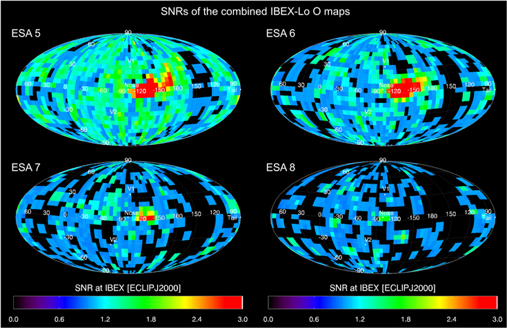
Figure 3. S/N values of the combined IBEX-Lo heavy neutral maps in energy channels 5–8. The map projection style and legends are the same as the map style and legends in Figure 1.
Download figure:
Standard image High-resolution imageThe S/N filter was applied to the combined IBEX-Lo heavy neutral maps. The first column of Figure 4 shows the S/N filtered maps in the top four energy channels (ESA 5–8). In the S/N filtered maps, an enhanced region of heavy neutral atoms emerges on the right-hand side (λ = 180° – 196° and β = +6° – +24°) of the ISN gas flow in the maps in energy channels 5 (0.279 keV) and 6 (0.601 keV). We refer to this enhanced region as the extended tail, which corresponds to the oxygen tail mentioned in Section 2.4. In the map in energy channel 7, the ISN gas flow is still visible but the extended tail is not present. Also, we could not find any relevant emissions in the map in energy channel 8. The extended tail will be discussed in Section 4 in more detail.

Figure 4. Sky maps in which the three statistical methods were applied: the S/N filter (left), the CLM (middle), and the cluster method (right). The S/N filtered maps show the count rates in pixels with S/N values exceeding a threshold. The CLM maps represent the upper confidence limits for CL = 84.13%. The cluster maps illustrate the cluster IDs, which correspond to the counts per hour. The four rows correspond to the top four energy channels from 0.279 to 2.361 keV. The map projection style and legends are the same as the map style and legends in Figure 1. See the text for further explanations.
Download figure:
Standard image High-resolution image3.2. The CLM
The so-called CLM provides the statistical significance for the count rates in a particular pixel and its neighboring pixels in a map. To define the statistical significance, we consider the upper (λu) and lower (λl) limits of the confidence level (CL). The CL is the probability that the actually observed number of counts N falls between the upper and lower limits. In a measured count map, the measured number of counts N in a pixel represents a single sample of possible measurements taken from a parent probability distribution. The average value of the parent distribution is a quantity which we attempt to determine. If we could observe the viewing direction of each pixel for a long period, then we could determine the parent distribution and obtain the desired value of our measured quantity very exactly. A finite set of measurements only allows us to estimate the average value with uncertainty, which can be expressed in terms of upper and lower limits. Based on Poisson statistics, the upper and lower limits are defined as

where N is the number of measured counts (Gehrels 1986). Since these formulas cannot be derived as exact algebraic expressions, we use the analytic approximations to calculate the limits, which were derived by Gehrels (1986).
In the measured count maps, due to the different exposure times in each pixel, we cannot directly compare the numbers of measured counts among pixels. Therefore, we calculate the count rates for pixels as written in Section 2.4. To obtain reasonable statistics, we now estimate the number of counts (C'(i, j)) measured with an identical exposure time, one hour, in each pixel. Using Equation (2), we then attempted to determine the upper and lower limits of the expected counts in particular pixels and their neighboring pixels with a specified CL (e.g., CL = 84.13%, which corresponds to a 1σ Gaussian error). The neighboring pixels should be located within a specified radius (12° = 2 pixels in this study) around each particular pixel. We call these pixels the test region for each particular pixel. Here, we should keep in mind that these upper and lower limits are the confidence interval for the sum of the expected counts in the test region. We eventually would like to express the statistical significance of the count rates in each pixel as upper and lower confidence limits. Thus, we divide these two limits by the number of pixels in the test region (Ntest) and 3600 s:  and
and  The desired count rate measured in the particular pixel should be within these upper and lower limits (
 ) with CL. After that step, we repeat this procedure for every pixel in the map.
Gehrel's analytic approximations used in the CLM do not consider the case of nonzero background. Therefore, we need to extend the CLM to a situation in which the statistical fluctuations in the background cannot be neglected. One way to extend the CLM to the cases with nonzero background is to subtract an average background count rate from the confidence limits calculated in the previous paragraph. In the combined IBEX-Lo heavy neutral maps, we assume that the pixels with an S/N less than 1.0 do not have a statistical significance. Therefore, we treat them as background pixels. The average background count rate is the average count rate in these background pixels:  where the indices i'' and j'' indicate the longitude and latitude indices of the background pixels and Nb is the number of background pixels. These average values and their standard deviations are provided in Table 3.
Table 3. The Average Background Rates (b) of the Combined IBEX-Lo Heavy Neutral Maps in the Top Four Energy Channels with Standard Deviations (σb)
| ESA Channel | b (×10−4 cts s−1) | σb (×10−4 cts s−1) |
|---|---|---|
| 5 | 3.66 ± 0.26 | 4.07 |
| 6 | 2.32 ± 0.82 | 1.60 |
| 7 | 1.70 ± 0.04 | 8.14 |
| 8 | 1.54 ± 0.05 | 8.05 |
Download table as: ASCIITypeset image
The second column in Figure 4 shows the upper confidence limits of the combined IBEX-Lo heavy neutral maps. These maps still include the average background count rates. Similar to the S/N-filtered maps, the extended tail is clearly present in the map of ESA step 5. The map of ESA 6 also shows the extended tail, but its intensity and extension are reduced. Figure 5 shows the upper confidence limits after subtracting the average background count rates. In these maps, the background pixels are removed and we can see the upper limits of count rates, which have valid statistical significance. We can also see that the same features are evident in the S/N-filtered maps. The visible features will be discussed in Section 4 in more detail.

Figure 5. Upper confidence limits (CL = 84.13%) of the combined IBEX-Lo heavy neutral maps after subtracting the average background count rates in the top four ESA energy channels (ESA 5–8). The average background count rates of the four energy channels are in Table 3. The map projection style and legends are the same as the map style and legends in Figure 1.
Download figure:
Standard image High-resolution image3.3. The Cluster Analysis Method
In this section, we describe the cluster analysis method, which defines groups of pixels in a map that contain similar count rates. Unlike the previous two statistical methods, this method does not directly address the statistical significance of the count rates in each pixel. However, by comparing them with this method, we can test whether or not the previous two methods show reasonable features in maps that extend over several pixels.
The main idea is the same as in density-based clustering (chapter 8 in Tan et al. 2005), which locates regions of high density that are separated from one another by regions of low density. In the combined IBEX-Lo heavy neutral maps, instead of the density, we consider count rates in neighboring pixels within a specific radius of a selected center pixel. The selected pixel cluster includes the center pixel and all of the neighboring pixels. The main algorithm works as follows. For a center pixel ( ), we add up the count rates in the neighboring pixels within a specific radius (
 ) of the center pixel:
  where
where  and
and  indicates the location of one of the neighboring pixels. In this study, the specific radius was chosen as one pixel because if we chose two pixels or more for the specific radius, the cluster method would fail to produce relevant clusters or groups in the combined IBEX-Lo heavy neutral maps. If the sum of the count rates is larger than a given local count rate per cluster (Clocal), then the pixel at
  is identified as a core pixel of the cluster (
 ). If the summed count rate is lower than a given local rate, then the pixel at
  is identified as a noise pixel (
 ). We then repeat the same procedure for all of the pixels to see if the pixel belongs to the core or not until noise pixels are encountered.
The third column in Figure 4 shows the heavy neutral atom sky maps after application of the cluster method. The colors in these maps indicate the cluster IDs, which correspond to count rates per hour (cts hr−1). In the ESA 5 sky map, the pixels with Cluster IDs 5 and 6 (5 cts hr−1 and 6 cts hr−1, blue pixels) are distributed in the tail to the upper right of the ISN gas flow. The ISN gas flow is indicated as Cluster ID 10 because it contains significantly higher count rates than any other pixels. Therefore, the cluster method is good for true signals, which agree well with the other two statistical methods. Even though this method does not provide the statistical significance, it strongly supports these two visible features being relevant.
4. DISCUSSION
In this section, we discuss two observable features (the ISN O&Ne gas flow and the extended tail) that are visible in the combined IBEX-Lo heavy neutral maps and supported by three statistical analysis methods. These two features are summarized in Figure 6 with contour lines. In particular, we focus on the extended tail. Figure 6(A) shows the upper confidence limits (CL = 84.13%) of the combined IBEX-Lo heavy neutral map after subtracting the average background count rate in energy channel 5 in a rectangular projection with contour lines. This map is identical to the upper left panel of Figure 5. The contour lines correspond to 0.001, 0.002, 0.005, 0.01, and 0.015 cts s−1 from the outer line to the inner line. Figure 6(B) illustrates the upper limits of the heavy neutral fluxes in the solar inertial frame in energy channel 5. This large flux map only shows the nose direction (λ = 180°–360°) to focus the two observable features in terms of fluxes in the solar inertial frame. The upper limits of the fluxes in the spacecraft frame are converted from the upper confidence limits of the combined count rates (Figure 6(A)) divided by the product of the center energy and the geometric factor: J = C/(E · G) (see Table 1). The fluxes in the solar inertial frame Jiner are related to the fluxes in the spacecraft frame J by the following relation: Jiner = EinerJ/E, where 

 is the velocity of the spacecraft, and
  is the velocity of the neutral atom in the spacecraft frame (McComas et al. 2010; Fuselier et al. 2012, 2014). The contour lines indicate fluxes of 15, 30, 60, 100, 150, and 180 cm−2 s−1 sr−1 keV−1.
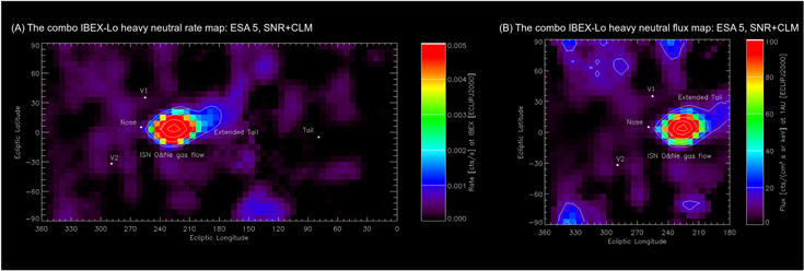
Figure 6. (A) The upper confidence limits (CL = 84.13%) of the combined IBEX-Lo heavy neutral map after subtracting the average background count rate in energy channel 5 in a rectangular projection with contour lines. This map is identical to the upper left panel of Figure 5. The contour lines correspond to 0.001, 0.002, 0.005, 0.01 and 0.015 cts s−1 from the outer line to the inner line. Here, we use the same color bar scale as in Figure 1. (B) The upper limits of heavy neutral fluxes in the solar inertial frame in energy channel 5, which is converted from the left panel (see text for detail). Here, we only show the nose direction (λ = 180°–360°) to show the ISN O&Ne gas flow and the extended tail in terms of the fluxes in the solar inertial frame. The contour lines indicate fluxes of 15, 30, 60, 100, 150, and 180 cm−2 s−1 sr−1 keV−1. The two major visible features (the ISN O&Ne gas flow and the extended tail) are labeled. The directions to the nose, tail, and the two Voyager spacecraft are marked with white circles.
Download figure:
Standard image High-resolution image4.1. Observable Features in the Oxygen Sky Maps
All three statistical analyses in this study corroborate each other and support the same statistically significant features in the oxygen maps. The most dominant feature in these maps is the ISN gas flow distribution, which is distributed from λ = 200° to 250° and from β = −12° to +20°, and is clearly identifiable within the energy range 0.2–1.2 keV (see Figures 4 and 6). Due to the Sun's gravitation, the ISN trajectories are deflected. Therefore, the observable direction is shifted from the nose direction. Using energy conservation, we calculate the expected ISN gas flow speed as a function of heliocentric radial distance r as  where
where  is the bulk speed of the ISN gas flow at infinity, Ms is the solar mass, and G is a gravitational constant. We ignore the effect of solar radiation pressure because it is negligible for heavy atoms such as O and Ne. For now, we adopt the flow speed at infinity as 26 km s−1 (McComas et al. 2015), resulting in VISM,1AU = 49 km s−1 in the Sun's rest frame at 1 AU. Since the Earth moves in the ram direction of the flow with VE ∼ 30 km s−1 in spring, the flow speed relative to the IBEX-Lo sensor is ∼79 km s−1. Thus, the bulk energies of ISN O and Ne are ∼530 eV and ∼660 eV, respectively. These bulk energies correspond to the energy range of energy channel 6 (see Table 1). Because incoming O atoms produce converted O−, and both O and Ne atoms produce sputtered O− and C− at lower energies, we conclude that the red regions in the maps in energy channels 5 and 6 represent the ISN O&Ne gas flow. Due to a wide energy acceptance (ΔE/E ≈ 0.7) of the electrostatic analyzer in the IBEX-Lo sensor, the ISN O&Ne gas flow can also be seen in the ESA 7 map. However, it cannot be observed in the map in the highest energy channel, channel 8. The three statistical analyses applied to the ESA 8 map confirm that there is no organized feature that can be associated with the O&Ne flow.
In these maps, the most interesting feature is the extended tail of heavy neutrals toward lower longitude and higher positive latitude (λ = 180°–200° and β = +5° – +25°) in the maps in energy channels 5 and 6 (see Figures 4 or 6). This extended tail persists in the maps to which the three different statistic methods have been applied. It is seen over the energy range 0.2–0.8 keV with the peak intensity at 0.279 keV, whereas it is not present at energies ≥1.2 keV. A similar feature was found in the observations of ISN He atoms, which is referred to as the Warm Breeze (Bzowski et al. 2012; Kubiak et al. 2014; Sokół et al. 2015). Kubiak et al. (2014) note that the flowing direction of the Warm Breeze is ∼20° away from the inflow direction of ISN He. This population is slower and warmer than the primary ISN He. Both the extended tail and the Warm Breeze are suspected to be imprints of the aforementioned secondary population. We will discuss the extended tail in more detail in Section 4.2.
4.2. The Extended Tail
The S/N filtered map in energy channel 5 shows that the peak of the extended tail is observed at λ ≈ 189° and β ≈ +15°, which is ∼36° away from the observed peak direction (λ ≈ 225° and β ≈ +3°) of the ISN O&Ne gas flow in Earth's orbit (see the upper left panel in Figure 4). To account for the extended tail, we compare the latitude profiles of the count rates for the swaths that include the ISN gas flow (λ = 200°–250°) and the extended tail (λ = 180°–200°) in the combined IBEX-Lo heavy neutral map in energy channel 5 (upper right panel in Figure 1). Using these profiles, we investigate the observed flow peak angles of the extended tail in latitude (Ψpeak) and their peak heights in count rate (Cmax), and then compare them with the ISN gas flow.
Figure 7 shows two examples of the latitude profiles corresponding to λ = 189° (left panel) and 225° (right panel) where the peaks of the extended tail and the ISN gas flow are observed, respectively. In these profiles, the blue circles represent the count rates corresponding to the extended tail or the ISN O&Ne gas flow (within ±3σ from the peak latitude). The black circles are the count rates outside the flows, which are used to estimate the background levels. The error bars are the standard deviations (σC) described in Section 2.4. Since these profiles show an asymmetric distribution, we used an exponentially modified Gaussian (EMG) function to determine the flow peak angles instead a Gaussian function. The EMG function is written as

where the parameter a0 is the area of the peak, a1 is the peak center, a2 is the standard deviation of the Gaussian component (width), and a3 is the exponential slope describing the asymmetry of the peak (distortion). The physical cause of the asymmetry is not completely understood, but it could be a sign of the secondary population represented as the extended tail in the combined IBEX-Lo heavy neutral maps. The red solid lines in Figure 7 represent the fit curves of the flow peak with the average background count rate in the combined IBEX-Lo heavy neutral map in energy channel 5. The average background count rate was determined in Section 3.2 (see Table 3).
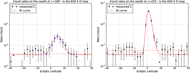
Figure 7. Count rates on the swaths corresponding to λ = 189° (λobs = 99°, in the left panel) and λ = 225° (λobs = 135°, in the right panel) in the combined IBEX-Lo heavy neutral map in energy channel 5 (upper right panel of Figure 1). The red solid lines are the EMG fit curves with the average background count rates for this map. The blue circles represent the flow count rates within ±3σ of the peak center. The black circles are count rates outside the flow, which are used to calculate the background levels of each swath. The red dashed horizontal lines indicate the background levels for the swath at λ = 189° and λ = 225°.
Download figure:
Standard image High-resolution imageFor each swath, there are two statistical variables: the maximum of the count rate (signal), Cmax, and the background level at the location of the signal maximum, Cbg. The maximum count rate is estimated through fitting the curve to all of the count rates on the swath. The background level is considered to be constant, and so it is represented by the average value of all of the count rates outside of the flow. We calculated the background levels for each swath  with standard deviation
  The uncertainty (error of the mean) is given by
  where Ci are the count rates represented as black circles in Figure 7 and n is the number of these data points. The background levels are shown as the horizontal red dashed lines in Figure 7 (also in Table 4).
Table 4. The Maximum Count Rates, the Background Levels, and the p-values of the Swaths from λ = 180° to λ = 246° in the Combined IBEX-Lo Heavy Neutral Map in Energy Channel 5
| λswath | Cmax |

|
Cbg |

|
p-value |
|---|---|---|---|---|---|
| (°) | (×10−3 cts s−1) | (×10−3 cts s−1) | (×10−3 cts s−1) | (×10−3 cts s−1) | (×10−4) |
| 183 | 2.03 | 0.99 | 0.30 | 0.18 | 2.112 |
| 189 | 2.79 | 0.87 | 0.40 | 0.21 | 2.113 |
| 195 | 1.99 | 0.73 | 0.40 | 0.17 | 2.115 |
| 201 | 2.96 | 0.99 | 0.42 | 0.20 | 2.113 |
| 207 | 4.40 | 1.65 | 0.62 | 0.25 | 2.108 |
| 213 | 11.81 | 2.52 | 0.57 | 0.33 | 2.108 |
| 219 | 33.44 | 3.43 | 0.54 | 0.43 | 2.111 |
| 225 | 42.60 | 3.48 | 0.58 | 0.27 | 2.111 |
| 231 | 40.88 | 4.85 | 0.68 | 0.37 | 2.110 |
| 237 | 24.76 | 2.57 | 0.57 | 0.20 | 2.110 |
| 243 | 6.34 | 1.35 | 0.45 | 0.19 | 2.111 |
Note. We also insert their standard deviations and characterizations. λswath is the center longitude of a swath.
Download table as: ASCIITypeset image
In Figure 8, we show the flow peak latitude (Ψpeak) of the extended tail and the ISN O&Ne gas flow as a function of the observer longitude λobs. The observer longitude corresponds to the location of the IBEX spacecraft, i.e., it is shifted 90° from the sensor view direction (λobs = λ − 90°). Here, we consider the flow peak latitude as the flow directions in latitude, and so they have negative values because we observe them above the ecliptic plane (Ψpeak = −βpeak). In an EMG function, a peak center does not indicate a peak position because of a distortion. Therefore, the peak positions in each swath are determined by the second derivative of the EMG function (d2C(β)/dβ2 = 0 at the peak position). We use the uncertainty of the parameter a1 ( ) as the uncertainty of the peak position. Then, the estimated peak positions are transformed to the flow peak latitudes and represented as red circles with their uncertainties. Two vertical blue lines indicate the maximum peaks of the extended tail (left line) and the ISN O&Ne gas flow (right line), respectively. For comparison, the flow peak latitudes of the ISN He gas flow are represented as black triangles and were determined by Leonard et al. (2015). They determined these flow peak latitudes through ISN He observations using the analytical model developed by Lee et al. (2012). The green solid line is the analytical model fit curve.

Figure 8. Latitude Ψpeak of the flow peaks as a function of observer longitude λobs. A latitude Ψpeak is a flow direction in latitude. The red circles are the flow peak latitudes of the ISN O&Ne gas flow and the extended tail. The values are estimated by fitting the measured count rates along each swath of the combined IBEX-Lo heavy neutral map in energy channel 5 with an EMG function. The black circles are the flow peak latitudes of the ISN He gas flow, which are estimated by the observation of He atoms with the analytical model (Leonard et al. 2015). The green solid line is the analytical model fit curve for the ISN He gas flow. The two blue vertical lines indicate the maximum peaks of the extended tail (λ = 189°, left) and the ISN O&Ne gas flow (λ = 225°, right), respectively.
Download figure:
Standard image High-resolution imageThe analytical model assumes that the ISN distribution is a drifting Maxwellian in the local interstellar medium with a flow speed at infinity. Under the Sun's gravitational field, the flow peak latitudes theoretically vary according to flow speeds, but do not strongly depend on species. If the heavy neutral observations show only the primary ISN O&Ne atoms with the same flow speed as the ISN He gas flow at infinity, the observed flow peak latitudes should follow the analytical model fit curve. Figure 8 shows that the interstellar heavy neutral observations qualitatively agree with the ISN He observations and the analytical model in the angular range λobs = 115°–160° where the ISN gas flow is observed. However, there is significant discrepancy between the interstellar heavy neutral observations and the analytical model fit curve where the observer longitude is less than ∼115°. This discrepancy shows that the extended tail is independent of the ISN O&Ne gas flow. Therefore, this extended tail is different for the interstellar He flow and might be identified as a secondary O population that has a different flow vector than the ISN O&Ne gas flow at infinity.
Figure 9 shows the maximum count rates (black circles) and background levels (blue triangles) for the swaths in the combined IBEX-Lo heavy neutral map in energy channels 5 (left panel) and 6 (right panel). The error bars of the maximum count rates are the standard deviations determined in Section 2.2. The error bars of the background levels are the standard deviations  For comparison, we also insert the blue horizontal lines, which indicate the average background count rates for the combined IBEX-Lo heavy neutral maps in energy channels 5 and 6. The background levels of each swath agree well with the average background count rates. We tried to fit these maximum count rates with two Gaussian functions, but the fit failed to converge. Here, we show two arbitrary Gaussian curves, which are close to the maximum count rates. In Figure 9, the red dashed lines represent these two Gaussian curves and the red solid line is the sum of two Gaussians. The two vertical red lines are the centers of these two Gaussian curves. The intensity of the extended tail is approximately 2%–4% of the peak of the ISN O&Ne gas flow, but it is three times greater than the background levels. Its intensity is much lower than the ISN O&Ne gas flow, but the p-values show that the intensity of the extended tail is significantly higher than the surrounding regions.

Figure 9. Peak count rates (black circles) and background levels (blue triangles) of heavy neutral atoms on the swaths corresponding to the ISN O&Ne gas flow and the extended tail in the combined IBEX-Lo heavy neutral map in energy channels 5 (left panel) and 6 (right panel). The two red vertical lines are the center longitudes of two arbitrary Gaussian curves (red dashed lines), which correspond to the longitude of the most intense pixel in the extended tail (left line) and the ISN O&Ne gas flow (right line), respectively. The red solid line is the superposition of these two Gaussian curves. The error bars of the peak count rates are standard deviations. The blue horizontal lines are the average background count rates for the combined IBEX-Lo heavy neutral maps in energy channels 5 and 6, which are described in Section 3.2.
Download figure:
Standard image High-resolution image
It is interesting to test the significance of the signal in each swath with p-values. One way to test this is by finding whether or not the null hypothesis is true. The statistical test is applied to the following null hypothesis: the maximum (peak) of the count rates and the background level (at the same location) belong to the same statistical population; namely, the signal is background. From the previous fitting, we can derive, for any swath, the following six values: the maximum of the count rates (Cmax), the uncertainty of the maximum ( ), the number of data points involved in the fitting of the count rates (
 ), the background level (Cbg), the uncertainty of the background level (
 ), and the number of data points involved in the averaging of the background level (
 ). Here, we use the standard deviations as the uncertainties of the maximum count rates and the background levels, respectively. We estimate the observed value tobs, which is supposed to follow a t-distribution with degrees of freedom νobs:


The t-distribution is as follows:

Then, the p-value is given by

If p-value >0.05, then the null hypothesis is accepted, meaning that the observed signal is likely background. The p-values are characterized by six characterizations according to Table 1 in Livadiotis (2014): impossible (p ∼ 0), highly unlikely (0<p<0.005), unlikely (0.005 p<0.05), likely (0.05
 p<0.19), highly likely (0.19
 p<0.5), and certain (p ∼ 0.5). We examined the p-values for each swath corresponding to the ISN gas flow and the extended tail in the combined IBEX-Lo heavy neutral map in energy channel 5. The calculated p-value is ∼0.0002, which means the null hypothesis is highly unlikely for all of the swaths that we investigate (see Table 4). In other words, these p-values show that the maximum values of the count rates for the extended tail are highly likely to be the real signal.
The most likely source of the extended tail may be a secondary population that is generated, at least at some level, by charge exchange between interstellar O+ ions and ISN H atoms in the outer heliosheath (in front of the heliopause). As the interstellar ions approach the heliopause, the ions are forced to flow around the heliopause and are heated (Izmodenov et al. 1997). A fraction of these ions obtain an electron from the interstellar atoms through charge exchange, and then become secondary oxygen atoms:  If we can observe these secondary oxygen atoms, then they should have lower bulk speeds than the primary ISN atoms because the parent ions are deflected around the heliopause. Due to the solar gravitational field, these slower atoms are deflected more than the primary neutral atoms as they approach Earth. Therefore, the secondary population should be observed in different regions (i.e., earlier orbits than the ISN gas flow from the end of December to the middle of January) in the map. To estimate the expected flux of the secondary oxygen atoms, we require a model to describe the mechanism of production and loss in the heliosheath and the heliosphere, but such an investigation is beyond the scope of this paper. However, all of these aspects are qualitatively consistent with our observations of the extended tail. The extended tail is most intense in the map at 0.279 keV, which is at a lower energy than the bulk energy of the ISN O&Ne gas flow, and the extended tail is observed 38° away from the peak of the gas flow. Figure 9 shows that the secondary peak of the count rates at λobs = 100° (λ ≈ 190°) is higher in ESA 5 than in ESA 6, whereas the primary peak of the count rates at λobs ≈ 137° (λ ≈ 227°) is higher in ESA 6 than in ESA 5.
5. CONCLUSIONS
We have studied the directional distribution of heavy neutral atoms in the IBEX-Lo heavy neutral maps generated from IBEX-Lo observations during 2009–2011. We combined the IBEX-Lo heavy neutral maps for three years to improve our statistics. To obtain a better understanding of the statistical significance of the count rates in the combined IBEX-Lo heavy neutral maps, we applied three statistical methods: the signal-to-noise filter, the CLM, and the cluster method. As a result, we found two consistent visible features: the ISN O&Ne gas flow and the extended tail (see Figure 6). We could not find any localized feature with statistical significance in the combined IBEX-Lo heavy neutral map of the top ESA channel (ESA8). Obviously, the ISN O&Ne gas flow is observed in the combined IBEX-Lo heavy neutral map at 0.601 keV, which corresponds to the bulk energies of the ISN O and Ne atoms. The ISN neutral gas flow is also observed at 0.279 and 1.206 keV because of the sputtered events and the wide energy band of the ESA, respectively. The more interesting feature in the combined IBEX-Lo heavy neutral maps is the extended tail, which is observed at 0.279 and 0.601 keV. The observed direction of the extended tail is around λ = 189° and β = +15°, which is ∼38° away from the peak of the ISN O&Ne gas flow, and the intensity is approximately 2%–4% of the maximum count rate of the ISN O&Ne gas flow. The extended tail is most intense at 0.279 keV and is still observable at 0.601 keV. However, it is not present in the two higher energy channels. This feature is likely an imprint of the secondary population created by charge exchange between interstellar ions and neutral atoms in front of the heliopause. A quantitative study of the fluxes of heavy neutral atoms, along with global simulations, of the heliosphere is required to further test the secondary population theory.
This work was supported by the Interstellar Boundary Explorer mission as a part of the NASA Explorer Program.