


ABSTRACT
The goal of the present work is to produce transition probabilities with very low uncertainties for a selected set of multiplets of Mn i and Mn ii. Multiplets are chosen based upon their suitability for stellar abundance analysis. We report on new radiative lifetime measurements for 22 levels of Mn i from the e8D, z6P, z6D, z4F, e8S, and e6S terms and six levels of Mn ii from the z5P and z7P terms using time-resolved laser-induced fluorescence on a slow atom/ion beam. New branching fractions for transitions from these levels, measured using a Fourier-transform spectrometer, are reported. When combined, these measurements yield transition probabilities for 47 transitions of Mn i and 15 transitions of Mn ii. Comparisons are made to data from the literature and to Russell–Saunders (LS) theory. In keeping with the goal of producing a set of transition probabilities with the highest possible accuracy and precision, we recommend a weighted mean result incorporating our measurements on Mn i and ii as well as independent measurements or calculations that we view as reliable and of a quality similar to ours. In a forthcoming paper, these Mn i/ii transition probability data will be utilized to derive the Mn abundance in stars with spectra from both space-based and ground-based facilities over a 4000 Å wavelength range. With the employment of a local thermodynamic equilibrium line transfer code, the Mn i/ii ionization balance will be determined for stars of different evolutionary states.
Export citation and abstract BibTeX RIS
1. INTRODUCTION
Elemental abundance determinations in stellar atmospheres have traditionally been based on one-dimensional (1D) atmospheric models and radiative transfer which incorporate the local thermodynamic equilibrium (LTE) approximation. Atomic transition probabilities and other laboratory spectroscopic data have been improved significantly in recent years. Consequently, for some species atomic data are no longer a significant source of error in stellar abundance analyses. There is growing interest in improving photospheric models and line transfer computations by incorporating more realistic treatments of radiation transport such as non-LTE and three dimensionality. The need for these more realistic treatments becomes urgent when controversy arises over an apparent abundance trend as a function of metallicity ([Fe/H];5 e.g., as found for the element manganese by Bergemann & Gehren 2008). Trends in abundance variations with metallicity caused by systematics in spectrum modeling and data reduction, such as unaccounted non-LTE (nLTE)/3D effects, residual errors in transition probabilities, and uncertain continuum placement, have to be clearly separated from the physics of nucleosynthesis. Abundance trends as a function of metallicity are used to establish both the astrophysical origin of a particular element and its nucleosynthetic history. Reduction of residual errors in transition probability data will assist in the unambiguous determination of elemental abundance trends. Note that the abundance behaviors as a function of metallicity do not mimic one another for elements of the Fe-peak and in some cases, depart significantly (e.g., McWilliam 1997). For example, with the employment of LTE line transfer codes, large-scale surveys of field and globular cluster stars have found that the [Co/Fe] ratio hovers roughly at its solar value over a two-order magnitude span in [Fe/H], whereas [Mn/Fe] exhibits a distinctly subsolar value over the same metallicity range (e.g., Gratton & Sneden 1991; Reddy et al. 2003, 2006; Sobeck et al. 2006). The accuracy of these trends is indeed an issue as nucleosynthetic yield calculations are still not able to reproduce observational data over the full range of metallicity. For example, Kobayashi et al. (2006) are not able to duplicate the behavior of [Mn i/Fe] in extremely metal-poor stars without the inclusion of nucleosynthetic input from a special class of supernovae called hypernovae.
Recent determinations of gf-values have been reported for Mn i by Blackwell-Whitehead et al. (2005a, 2005c) and Blackwell-Whitehead & Bergemann (2007). With these new data, Blackwell-Whitehead & Bergemann (2007) and Bergemann & Gehren (2007) found departures between the LTE- and nLTE-derived abundances for the neutral species of Mn in the Sun and suggested that the maximum amount of nLTE correction could be approximately +0.1 dex. These papers focused on the determination of Mn i oscillator strengths and examined the nLTE formation of Mn i transitions in the solar atmosphere. Our paper reports a new laboratory investigation that tests and extends the recent work on Mn i and includes Mn ii. The goal is to minimize uncertainties in transition probabilities for both Mn i and Mn ii lines so that the ionization balance may be examined in a variety of stellar evolutionary groups over a wide range of metallicity.
Our approach to lab work on Mn i and Mn ii is more selective than what we used in recent studies of rare earth ions (e.g., Lawler et al. 2009, and references therein) for which we measured transition probabilities for hundreds of lines for each ion. The current study in manganese is particularly focused on multiplets which are amenable to very accurate transition probability measurements and which are useful in abundance studies. In order to be satisfactory for abundance analysis, these transitions need to be relatively unblended in stellar spectra and have line strengths in a useful range. Of course, the optimum range of transition strength and excitation potential (E.P.) depends on the metallicity and effective temperature of the star. Astrophysical studies covering a wide range of metallicity thus require a selection of lines, all with the very accurate transition probabilities, covering a range of transition strength and/or E.P. Uncertainties of ±5% or 0.02 dex on radiative lifetime measurements are often dominated by larger uncertainties on branching fractions, which then yield log(gf) values with uncertainties >0.02 dex. Many comparisons (e.g., Lawler et al. 2008) indicate that radiative lifetimes measured using laser induced fluorescence (LIF) are accurate to ±5% or better. The use of atomic benchmark lifetimes to regularly perform an end-to-end test of our LIF experiment has been effective at suppressing systematic errors. Although progress has been made on branching fraction measurement techniques, the results are often still not as accurate as lifetime measurements and are affected by systematic uncertainties which are difficult to quantify (Lawler et al. 2008). Branching fraction uncertainties can be suppressed by choosing dominant lines in multiplets with a narrow wavelength spread. Branching fractions are defined to sum to 1.0, thus uncertainty migrates to weaker lines. Radiometric calibration difficulties are minimal over small wavelength ranges. Finally, we are looking for multiplets which either have recent branching fraction measurements using a powerful Fourier transform spectrometer (FTS), or are pure Russell–Saunders (LS) multiplets to provide redundancy.
There has been a substantial amount of work on transition probabilities for Mn i and Mn ii lines. The older, pre-1988 results are summarized in the NIST critical compilation (Martin et al. 1988). Direct comparison is made between our branching fraction results below and more recent FTS results in the literature. Simple theory can also be used to check our FTS measurements on pure LS multiplets. The final set of log(gf) values for Mn i and Mn ii (with reduced uncertainties) is sufficiently large to cover an ample range of transition strength and E.P. and, consequently, allow for an accurate and comprehensive determination of the ionization equilibrium in a large stellar data sample.
The paper is organized as follows. Section 2 describes the radiative lifetime measurements for Mn i and Mn ii, and the results are presented along with a comparison to other modern laser-based lifetime measurements. Section 3 describes the branching fraction measurements, including a detailed discussion of each multiplet included in this study and presents the results and comparison to data in the literature. This section also contains a table of recommended log10(gf) values. The Appendix includes a machine-readable table of complete hyperfine component patterns reconstructed from data from the literature. They are included here for the convenience of the reader or user.
2. RADIATIVE LIFETIME MEASUREMENTS
The radiative lifetimes of the upper levels in this study have been measured using time-resolved laser-induced fluorescence (TRLIF) on a slow beam of manganese atoms and ions. The apparatus and technique is described in detail in other publications (see, for example, Den Hartog et al. 2002 for a full description) and only an overview will be given here. The atom/ion beam is produced with a hollow cathode sputter source. A pulsed electrical discharge, operated with ∼10 A, 10 μs duration pulses in 0.4 torr argon, is used to sputter metal from the hollow cathode which is lined with manganin, an alloy containing 86% copper, 12% manganese, and 2% nickel. The hollow cathode is closed on one end except for a 1 mm hole, through which the metal species are differentially pumped into a scattering chamber held at ∼10−4 torr. This produces a beam containing both neutral and singly ionized manganese which is slow (∼105 cm s−1) and only weakly collimated. The setup and technique described below is identical whether the measurement is for a neutral or ion.
The atom/ion beam is crossed at right angles by a laser beam 1 cm below the bottom of the cathode. The laser used is a nitrogen laser pumped dye laser system, which is tunable over the range 205–720 nm with the use of frequency doubling crystals, is operated at 30 Hz repetition rate and has a pulse duration of ∼3 ns. More importantly for lifetime measurements, the pulse terminates abruptly so that fluorescence can be observed free from excitation. The laser pulse, which is used to selectively excite the level to be studied, is delayed relative to the current pulse in the discharge by ∼20–30 μs to allow for the transit time of the atoms/ions. Fluorescence is then collected in a direction mutually orthogonal to the laser and atom beams through a pair of fused silica lenses and focused onto the photocathode of an RCA 1P28A photomultiplier.
The laser is coarse tuned to within ∼1 Å of the desired transition by tilting the laser grating. A LIF spectrum is then recorded in a 5–10 Å region around the transition by changing the pressure of the enclosed volume surrounding the grating. This gives very precise and reproducible control of the laser wavelength. Line separations on the LIF spectrum can be measured to ±0.03 Å and lines are identified by comparison with the National Bureau of Standards line list (Meggers et al. 1975). Once the transition is correctly identified, the fluorescence decay is recorded with a Tektronix SCD1000 digitizer beginning after the laser has completely terminated. An average is taken of 640 fluorescence decays. Then the laser is tuned off-line and an average of 640 background traces is recorded. The data are then downloaded to a computer for analysis. The digitizer data are divided into two separate time intervals for analysis, each approximately 1.5 lifetimes in length. A decay time is determined in each interval by performing a least-squares fit to a single exponential on the background-subtracted fluorescence decay. Comparison of the decay times in the two regions gives a good indication of whether the decay is a clean exponential, or whether some systematic effect has rendered it non-exponential. The lifetime is determined by averaging five decay times for a given set of experimental conditions. The statistical scatter of the data is typically in the range of 0.1%–3%. The lifetime of each level is measured at least twice, using different transitions for laser excitation whenever possible. The resulting redundancy helps to ensure that the transitions used were identified correctly in the experiment and are free from blends.
There are a number of systematic effects that must be considered in the measurement of radiative lifetimes using TRLIF. These effects have been carefully studied and controlled. They are discussed in detail in Den Hartog et al. (2002), and will only briefly be mentioned here. Zeeman quantum beats are controlled in the experiment by zeroing the magnetic field to within ±0.02 G in the beam interaction region with the use of Helmholtz coils. Effects arising from the finite bandwidth of the electronics only begin to be appreciable for lifetimes under 3 ns, whereas the shortest lifetime reported herein is 3.88 ns. The atomic/ionic beam source used in these measurements produces a gas phase sample which has been tested repeatedly and shown to be optically thin and free from collisional deexcitation effects. Flight-out-of-view effects only become a concern for neutral lifetimes longer than 300 ns (or ion lifetimes longer than 100 ns, because of their higher velocities). This is not a concern in the present set of measurements, as the longest neutral lifetime reported here is 65.9 ns, and the lifetimes of the six ion levels in this study are on the order of 4 ns.
Even with a full understanding of the systematic effects that enter into a particular measurement technique, it is still often difficult to accurately quantify the uncertainties that arise from those effects. To this end, we routinely put our apparatus and technique through an end-to-end test by measuring a series of cross check lifetimes in order to ensure that our reported lifetimes lie within the stated uncertainty. These are lifetimes which are well known from other sources, either very accurate calculations or measurements which have uncertainties significantly smaller than for our experiment. To cover the range of lifetimes in the present study, we have measured the following cross checks: z6D9/2 state of Fe ii at 3.70(6) ns (laser-fast beam measurement; Biémont et al. 1991), 22P3/2 state of Be+ at 8.8519(8) ns (variational method calculation; Yan et al. 1998), 4p'[1/2]1 state of Ar at 27.85(7) ns (beam-gas-laser-spectroscopy; Volz & Schmoranzer 1998), and 33P state of neutral He at 94.7 ns (variational method calculation; Kono & Hattori 1984). We have also added two new cross checks for this study in order to further quantify our systematic uncertainties. They are the 32P3/2 state of Mg+ at 3.85 ns (accuracy of ⩽1% at 90% confidence level) and the 32P3/2 state of neutral Na at 16.23(1) ns (accuracy of ⩽0.1% at 90% confidence level). Both the Mg+ and neutral Na cross checks are taken from the recent NIST critical compilation of Kelleher & Podobedova (2008). These cross check measurements are made with exactly the same apparatus and technique as the manganese measurements, except that the metal lining the cathode or, in the case of the helium cross checks, the gas in the discharge, is different. To produce a sodium component in the atomic beam, we run a high DC current (150 mA) which heats the anode assembly and drives sodium out of the Pyrex glass.
Careful attention to controlling the systematic effects mentioned above and the regular measurement of cross check lifetimes allow us to measure lifetimes routinely to ±5%, which is the uncertainty we have typically quoted for lifetimes measured with this apparatus. This has been shown to be a conservative estimate, representing closer to a "2σ" uncertainty than "1σ" (Lawler et al. 2008). This, in addition to the two new very accurate cross checks, gives us confidence that the uncertainties of the current lifetime measurements are within ±3%.
The results of our Mn i and ii lifetime measurements are given in Table 1. Comparison is made to experimental lifetime data in the literature measured using modern, laser-based techniques. Older measurements from less reliable methods are not included in Table 1. There is generally very good agreement among all these modern measurements. Figure 1 illustrates the level of agreement with a plot of the percent difference between our results and others (in the sense of (others−ours/ours) versus our lifetime. Specifically, we see the best agreement between our results and those of the three most recent TRLIF studies of Blackwell-Whitehead et al. (2005c, henceforth BW05), Kling et al. (2001, henceforth KSG01), and Schnabel et al. (1995, henceforth SBK95). The mean and rms differences between our lifetimes and theirs are −0.5% and 2.4%, respectively, for six measurements of BW05; +0.9% and 2.4%, respectively, for three measurements of KSG01; and +0.2% and 2.8%, respectively, for 19 measurements of SBK95. The agreement with the LIF-delayed coincidence work of Becker et al. (1980) is nearly as good (henceforth Be80; with mean and rms differences of −2.2% and 2.3%, respectively, for six measurements) and Kwiatkowski et al. (1982, henceforth Kw82; mean and rms differences of +2.4% and 3.1%, respectively, for five measurements). In the comparisons listed above, all of the lifetimes agree within the combined uncertainties of the two measurements. We see somewhat weaker but still very good agreement with the laser-fast beam measurements of Pinnington et al. (1992, henceforth Pi92). Mean and rms differences between our lifetimes and theirs are +2.3% and 3.8%, respectively, for the six short-lived Mn+ levels, and the combined uncertainties for the z5P3 lifetime does not quite cover the difference between our respective results for that level. Our results overlap with the LIF-delayed coincidence work of Marek (1975, henceforth Ma75) for two levels of neutral Mn. The mean and rms differences for these two levels are +5.5% and 12.8%, respectively, and only one of the two lifetimes agree within the combined uncertainties.
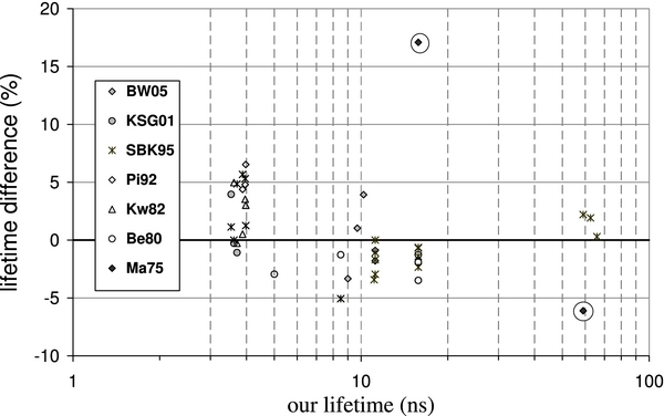
Figure 1. Comparison of our radiative lifetimes to those from the literature. The circled data points have been left out of the final recommended lifetime results because of their large uncertainties. See Table 1 footnote for list of references.
Download figure:
Standard image High-resolution imageTable 1. Radiative Lifetimes from LIF Measurements for Selected Levels of Mn i and ii
| Configuration | Levela | J | Laser Wavelengthb | Lifetimes from LIF Measurements | |||
|---|---|---|---|---|---|---|---|
| and Terma | (cm−1) | (Å) | This Expt. | Other Expt | Ref. | Recommended | |
| (ns) | (ns) | (ns) | |||||
| 3d54s(7S)4d e8D | 46706.09 | 1.5 | 3532.11 | 6.05 ± 0.18 | 6.05 ± 0.18 | ||
| 3d54s(7S)4d e8D | 46707.03 | 2.5 | 3531.99, 3548.18 | 6.02 ± 0.18 | 6.02 ± 0.18 | ||
| 3d54s(7S)4d e8D | 46708.33 | 3.5 | 3531.83, 3548.02 | 6.07 ± 0.18 | 6.07 ± 0.18 | ||
| 3d54s(7S)4d e8D | 46710.15 | 4.5 | 3547.79, 3569.80 | 6.04 ± 0.18 | 6.04 ± 0.18 | ||
| 3d54s(7S)4d e8D | 46712.58 | 5.5 | 3569.49 | 6.10 ± 0.18 | 6.10 ± 0.18 | ||
| 3d6(5D)4p x6P | 44993.92 | 3.5 | 2221.83, 3629.73 | 9.0 ± 0.3 | 8.7 ± 0.4 | BW05 | 8.9 ± 0.3 |
| 3d6(5D)4p x6P | 45156.11 | 2.5 | 2213.85, 3623.78 | 9.7 ± 0.3 | 9.8 ± 0.4 | BW05 | 9.7 ± 0.3 |
| 3d6(5D)4p x6P | 45259.17 | 1.5 | 2208.81, 3619.27 | 10.2 ± 0.3 | 10.6 ± 0.5 | BW05 | 10.3 ± 0.3 |
| 3d5(6S)4s4p(3P) z6P | 24802.25 | 3.5 | 4030.75 | 59.0 ± 1.8 | 60.3 ± 1.3 | SBK95 | 59.4 ± 1.6 |
| 55.4 ± 5.5 | Ma75 | ||||||
| 3d5(6S)4s4p(3P) z6P | 24788.05 | 2.5 | 4033.06 | 62.6 ± 1.9 | 63.8 ± 1.4 | SBK95 | 63.0 ± 1.7 |
| 3d5(6S)4s4p(3P) z6P | 24779.32 | 1.5 | 4034.48 | 65.9 ± 2.0 | 66.1 ± 1.4 | SBK95 | 66.0 ± 1.7 |
| 3d6(5D)4p z6D | 42198.56 | 0.5 | 4058.93, 4070.28 | 11.2 ± 0.3 | 11.08 ± 0.31 | SBK95 | 11.2 ± 0.3 |
| 3d6(5D)4p z6D | 42143.57 | 1.5 | 4048.74, 4079.41 | 11.2 ± 0.3 | 11.0 ± 0.5 | BW05 | 11.2 ± 0.4 |
| 11.20 ± 0.49 | SBK95 | ||||||
| 3d6(5D)4p z6D | 42053.73 | 2.5 | 4035.72, 4082.94 | 11.2 ± 0.3 | 11.0 ± 0.5 | BW05 | 11.1 ± 0.3 |
| 11.01 ± 0.27 | SBK95 | ||||||
| 3d6(5D)4p z6D | 41932.64 | 3.5 | 4055.54, 4083.63 | 11.2 ± 0.3 | 11.1 ± 0.5 | BW05 | 11.1 ± 0.3 |
| 10.87 ± 0.24 | SBK95 | ||||||
| 3d6(5D)4p z6D | 41789.48 | 4.5 | 4041.35, 4079.24 | 11.1 ± 0.3 | 10.72 ± 0.29 | SBK95 | 11.0 ± 0.3 |
| 3d6(5D)4p z4F | 44288.76 | 4.5 | 4762.37, 5255.33 | 15.8 ± 0.5 | 15.69 ± 0.33 | SBK95 | 15.6 ± 0.5 |
| 15.25 ± 0.7 | Be80 | ||||||
| 3d6(5D)4p z4F | 44523.45 | 3.5 | 4709.71, 4766.42 | 15.8 ± 0.5 | 15.70 ± 0.41 | SBK95 | 15.7 ± 0.5 |
| 15.6 ± 0.7 | Be80 | ||||||
| 3d6(5D)4p z4F | 44696.29 | 2.5 | 4727.46, 4765.85 | 15.8 ± 0.5 | 15.58 ± 0.37 | SBK95 | 15.7 ± 0.5 |
| 15.5 ± 0.7 | Be80 | ||||||
| 3d6(5D)4p z4F | 44814.73 | 1.5 | 4739.09, 4761.51 | 15.8 ± 0.5 | 15.43 ± 0.56 | SBK95 | 15.7 ± 0.6 |
| 15.6 ± 0.8 | Be80 | ||||||
| 3d54s(7S)5s e8S | 39431.31 | 3.5 | 4783.43, 4823.52 | 8.5 ± 0.3 | 8.07 ± 0.19 | SBK95 | 8.3 ± 0.3 |
| 8.25 ± 0.4 | Be80 | ||||||
| 3d54s(7S)5s e6S | 41403.93 | 2.5 | 4370.87 | 15.8 ± 0.5 | 18.5 ± 1.8 | Ma75 | 15.8 ± 0.5 |
| 3d5(6S)4p z5P | 43557.14 | 1 | 2933.06 | 3.88 ± 0.12 | 4.10 ± 0.16 | SBK95 | 3.98 ± 0.12 |
| 4.05 ± 0.10 | Pi92 | ||||||
| 3.9 ± 0.3 | Kw82 | ||||||
| 3d5(6S)4p z5P | 43484.64 | 2 | 2939.31 | 3.96 ± 0.12 | 4.17 ± 0.18 | SBK95 | 4.08 ± 0.12 |
| 4.15 ± 0.10 | Pi92 | ||||||
| 4.1 ± 0.3 | Kw82 | ||||||
| 3d5(6S)4p z5P | 43370.51 | 3 | 2949.20 | 3.98 ± 0.12 | 4.03 ± 0.11 | SBK95 | 4.09 ± 0.12 |
| 4.24 ± 0.10 | Pi92 | ||||||
| 4.1 ± 0.3 | Kw82 | ||||||
| 3d5(6S)4p z7P | 38366.18 | 2 | 2605.69 | 3.71 ± 0.11 | 3.67 ± 0.04 | KSG01 | 3.72 ± 0.11 |
| 3.89 ± 0.21 | SBK95 | ||||||
| 3.66 ± 0.05 | Pi92 | ||||||
| 3.7 ± 0.4 | Kw82 | ||||||
| 3d5(6S)4p z7P | 38543.08 | 3 | 2593.73 | 3.62 ± 0.11 | 3.61 ± 0.06 | KSG01 | 3.61 ± 0.10 |
| 3.62 ± 0.16 | SBK95 | ||||||
| 3.60 ± 0.05 | Pi92 | ||||||
| 3.8 ± 0.4 | Kw82 | ||||||
| 3d5(6S)4p z7P | 38806.67 | 4 | 2576.10 | 3.54 ± 0.11 | 3.68 ± 0.07 | KSG01 | 3.57 ± 0.09 |
| 3.58 ± 0.12 | SBK95 | ||||||
| 3.54 ± 0.05 | Pi92 | ||||||
Notes. aConfiguration, term, and energy levels from Sugar & Corliss (1985). bWavelength values computed from energy levels using the standard index of air from Peck & Reeder (1972). References. BW05: Blackwell-Whitehead et al. 2005a; SBK95: Schnabel et al. 1995; Ma75: Marek 1975; Be80: Becker et al. 1980; Kw82: Kwiatkowski et al. 1982; Pi92: Pinnington et al. 1992; KSG01: Kling et al. 2001.
Download table as: ASCIITypeset image
The final column of Table 1 lists a recommended value for the lifetime of each level. For the e8D multiplet this is our lifetime, and for the other levels it is a weighted average of our lifetimes and the other results listed in Table 1 except for those of Ma75. We have omitted Ma75's lifetimes from the average because of the large uncertainties quoted (10%) and the sense that in this early work, the systematics of the measurement may not have been completely under control. We have also omitted the results of Kw82 for the 3d5(6S)4p z7P2,3 levels of Mn ii because they have substantially higher uncertainties than the other available measurements for those levels. The weighting for the recommended averages is this: present work, x2; BW05, x1; SBK95, x1; Be80, x1; Kw82, x1; Pi92, x2; and KSG01, x1. We have weighted our results heavier than the other LIF results because of our measurement of cross checks, which allows us to quantify and correct for our residual systematic uncertainties. We have given the work of Pi92 a higher weighting than the LIF work and an equivalent weighting with our own because, for the short lifetimes (4 ns) measured by Pi92, the laser-fast beam technique should, in principle, be less prone to systematic effects than TRLIF.
3. BRANCHING FRACTION MEASUREMENTS
3.1. Description of Experiment
This experiment, like the recent work by Blackwell-Whitehead et al. (2005c) and Blackwell-Whitehead & Bergemann (2007), relies primarily on FTS data for the measurement of emission branching fractions. The high spectral resolving power and superb wavenumber accuracy of data from FTS instruments are major advantages for branching fraction measurements in complex spectra. The broad spectral coverage, large etendue, high data collection rates, and ability to record an entire spectrum in parallel are additional advantages. As in most of our earlier work, we use data from the 1.0 m FTS at the National Solar Observatory (NSO) on Kitt Peak for Mn i and Mn ii branching fraction measurements (Brault 1976). Although we are working over relatively small spectral ranges, radiometric calibration is necessary. We rely on the calibration provided by overlapping sets of Ar i and Ar ii lines, which are internal to the Mn/Ar hollow cathode discharge (HCD) lamp spectra. The Ar line method captures the wavelength-dependent response of detectors, spectrometer optics, lamp windows, and any other components in the light path or any reflections which contribute to the detected signal (such as due to light reflecting off the back of the hollow cathode). This calibration technique is based on a comparison of well-known branching ratios for sets of Ar i and Ar ii lines widely separated in wavelength, to the intensities measured for the same lines. Sets of Ar i and Ar ii lines have been established for this purpose in the range of 4300–35000 cm−1 by Adams & Whaling (1981), Danzmann & Kock (1982), Hashiguchi & Hasikuni (1985), and Whaling et al. (1993). Measurements from an echelle grating spectrometer in our lab are used to supplement and improve results from the FTS data for a few lines.
Five FTS spectra from the NSO electronic archives are used in this study.6 The first two of these are serial 2 and 3 recorded on 1980 September 4 using Mn/Ar HCD lamps operated at 150 mA. Spectrum 2 covers the region from 7965 to 40751 cm−1 with a limit of resolution of 0.061 cm−1. Spectrum 3 covers the region from 14975 to 37584 cm−1 with a limit of resolution of 0.048 cm−1. Both spectra have eight co-adds and both were recorded using the UV beam splitter. The Super Blue silicon photodiodes with Corning 9–54 dye filters were employed to record spectrum 2, while the midrange silicon photodiodes with CuSO4 and WG295 filters were employed to record spectrum 3. Spectrum 3 has slightly better signal-to-noise ratio (S/N) in the visible and UV from suppression of the multiplex noise due to strong near-IR lines of Ar i, but both spectra have high S/N for all but weak lines in this study.
A series of three spectra, serial 2–4, recorded on 1985 July 22 from an inductively coupled plasma (ICP) source with the Mn content stepped from 1 to 10 to 100 ppm are also used in this study. All three spectra in this series have four co-adds and cover the region from 14886 to 36998 cm−1 with a limit of resolution of 0.071 cm−1. The midrange silicon photodiodes with CuSO4 filters were employed to record the series. These ICP spectra are valuable for addressing concerns about possible optical depth errors since they cover such a large range of Mn density. These spectra do not have Ar emission lines and thus were radiometrically calibrated using another method. A calibration is established over narrow spectral regions from other archived spectra recorded a short time after the Mn spectra using the exact same FTS configuration.
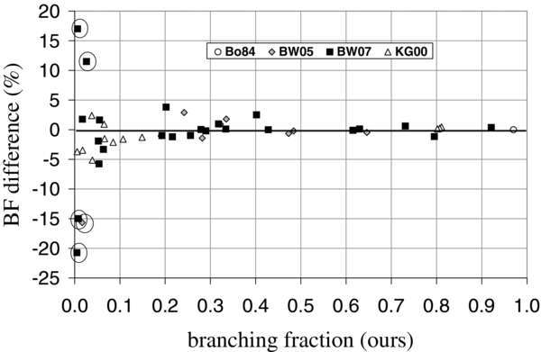
The results of our FTS branching fraction measurements are given in Table 2. Each multiplet included in this study is discussed below in some detail. Table 2 also compares our branching fractions to other recent FTS measurements or to LS coupling theory. The other experiments to which we compare use similar instruments and technique but represent different sources of data than ours. Figure 2 shows the percent difference between our branching fractions and others (in the sense (others − ours)/ours) versus our branching fractions. The circled data points are weak lines (discussed below) which have been left out of the final recommended log10(gf) results because of their large uncertainties. The goal is a set of branching fractions which have uncertainties <±5% with high confidence.
Figure 2. Comparison of our branching fractions to those from the literature. The circled data points are weak lines (see the text for discussion) which have been left out of the final recommended log10(gf) results because of their large uncertainties. See Table 2 notes for list of references.
Download figure:
Standard image High-resolution image
Table 2. Branching Fraction Measurements for Lines of Mn i (half-integral J) and Mn ii (integral J) from this FTS Experiment, Other Recent FTS Experiments, and LS Theory with Scaling
| Wave-Numbera | Wave-Lengthb | Upper Level | Lower Level | Branching Fractions from FTS Data | Branching Fractions | Branching Fractions | ||||||||
|---|---|---|---|---|---|---|---|---|---|---|---|---|---|---|
| Term | Energy | J | Term | Energy | J | This Experiment | Other Experiment | LS Theory | Recommended | |||||
| (cm−1) | (Å) | (cm−1) | (cm−1) | % Unc. | % Unc. | Ref. | ||||||||
| 28303.63 | 3532.11 | e8D | 46706.09 | 1.5 | z8P | 18402.46 | 2.5 | 1.000 | 2 | 1.0000 | 1.000 | |||
| 28304.57 | 3531.99 | e8D | 46707.03 | 2.5 | z8P | 18402.46 | 2.5 | 0.637 | 2 | 0.6460 | 0.642 | |||
| 28175.39 | 3548.18 | e8D | 46707.03 | 2.5 | z8P | 18531.64 | 3.5 | 0.363 | 2 | 0.3540 | 0.358 | |||
| 28305.87 | 3531.83 | e8D | 46708.33 | 3.5 | z8P | 18402.46 | 2.5 | 0.281 | 3 | 0.2710 | 0.276 | |||
| 28176.69 | 3548.02 | e8D | 46708.33 | 3.5 | z8P | 18531.64 | 3.5 | 0.616 | 2 | 0.6337 | 0.625 | |||
| 28002.96 | 3570.03 | e8D | 46708.33 | 3.5 | z8P | 18705.37 | 4.5 | 0.103 | 8 | 0.0953 | 0.099 | |||
| 28178.51 | 3547.79 | e8D | 46710.15 | 4.5 | z8P | 18531.64 | 3.5 | 0.610 | 2 | 0.6155 | 0.613 | |||
| 28004.78 | 3569.80 | e8D | 46710.15 | 4.5 | z8P | 18705.37 | 4.5 | 0.390 | 2 | 0.3845 | 0.387 | |||
| 28007.21 | 3569.49 | e8D | 46712.58 | 5.5 | z8P | 18705.37 | 4.5 | 1.000 | 2 | 1.0000 | 1.000 | |||
| 24802.25 | 4030.75 | z6P | 24802.25 | 3.5 | a6S | 0.00 | 2.5 | 0.970 | 2 | 0.97 | Bo84 | 0.97 | ||
| 24788.05 | 4033.06 | z6P | 24788.05 | 2.5 | a6S | 0.00 | 2.5 | 0.970 | 2 | 0.97 | ||||
| 24779.32 | 4034.48 | z6P | 24779.32 | 1.5 | a6S | 0.00 | 2.5 | 0.970 | 2 | 0.97 | ||||
| 24630.08 | 4058.93 | z6D | 42198.56 | 0.5 | a6D | 17568.48 | 1.5 | 0.795 | 1 | 0.7858 | BW07 | 0.790 | ||
| 24561.41 | 4070.28 | z6D | 42198.56 | 0.5 | a6D | 17637.15 | 0.5 | 0.202 | 2 | 0.2097 | BW07 | 0.206 | ||
| 24692.05 | 4048.74 | z6D | 42143.57 | 1.5 | a6D | 17451.52 | 2.5 | 0.646 | 1 | 0.643 | 11 | BW05 | 0.645 | |
| 24575.09 | 4068.01 | z6D | 42143.57 | 1.5 | a6D | 17568.48 | 1.5 | 0.0166 | 9 | 0.014 | 11 | BW05 | ||
| 24506.42 | 4079.41 | z6D | 42143.57 | 1.5 | a6D | 17637.15 | 0.5 | 0.335 | 1 | 0.341 | 11 | BW05 | 0.338 | |
| 24771.73 | 4035.72 | z6D | 42053.73 | 2.5 | a6D | 17282.00 | 3.5 | 0.484 | 1 | 0.483 | 6 | BW05 | 0.484 | |
| 24602.21 | 4063.53 | z6D | 42053.73 | 2.5 | a6D | 17451.52 | 2.5 | 0.191 | 1 | 0.189 | 6 | BW05 | 0.190 | |
| 24485.25 | 4082.94 | z6D | 42053.73 | 2.5 | a6D | 17568.48 | 1.5 | 0.322 | 1 | 0.325 | 6 | BW05 | 0.324 | |
| 24880.35 | 4018.10 | z6D | 41932.64 | 3.5 | a6D | 17052.29 | 4.5 | 0.282 | 1 | 0.278 | 5 | BW05 | 0.280 | |
| 24650.64 | 4055.54 | z6D | 41932.64 | 3.5 | a6D | 17282.00 | 3.5 | 0.473 | 1 | 0.470 | 5 | BW05 | 0.472 | |
| 24481.12 | 4083.63 | z6D | 41932.64 | 3.5 | a6D | 17451.52 | 2.5 | 0.242 | 1 | 0.249 | 5 | BW05 | 0.246 | |
| 24737.19 | 4041.35 | z6D | 41789.48 | 4.5 | a6D | 17052.29 | 4.5 | 0.858 | 1 | 0.858 | ||||
| 24507.48 | 4079.24 | z6D | 41789.48 | 4.5 | a6D | 17282.00 | 3.5 | 0.139 | 1 | 0.139 | ||||
| 20992.09 | 4762.37 | z4F | 44288.76 | 4.5 | a4D | 23296.67 | 3.5 | 0.921 | 1 | 0.9245 | BW07 | 0.923 | ||
| 19023.02 | 5255.33 | z4F | 44288.76 | 4.5 | a4G | 25265.74 | 5.5 | 0.0538 | 3 | 0.0507 | BW07 | 0.0523 | ||
| 19003.33 | 5260.77 | z4F | 44288.76 | 4.5 | a4G | 25285.43 | 4.5 | 0.0049 | 10 | 0.0039 | BW07 | |||
| 21226.78 | 4709.71 | z4F | 44523.45 | 3.5 | a4D | 23296.67 | 3.5 | 0.193 | 1 | 0.1911 | BW07 | 0.192 | ||
| 20974.25 | 4766.42 | z4F | 44523.45 | 3.5 | a4D | 23549.20 | 2.5 | 0.731 | 1 | 0.7355 | BW07 | 0.733 | ||
| 19238.02 | 5196.59 | z4F | 44523.45 | 3.5 | a4G | 25285.43 | 4.5 | 0.0523 | 3 | 0.0513 | BW07 | 0.0518 | ||
| 19235.71 | 5197.22 | z4F | 44523.45 | 3.5 | a4G | 25287.74 | 3.5 | 0.0081 | 10 | 0.0069 | BW07 | |||
| 21399.62 | 4671.67 | z4F | 44696.29 | 2.5 | a4D | 23296.67 | 3.5 | 0.0170 | 10 | 0.0173 | BW07 | 0.0172 | ||
| 21147.09 | 4727.46 | z4F | 44696.29 | 2.5 | a4D | 23549.20 | 2.5 | 0.2792 | 1 | 0.2793 | BW07 | 0.279 | ||
| 20976.77 | 4765.85 | z4F | 44696.29 | 2.5 | a4D | 23719.52 | 1.5 | 0.630 | 1 | 0.6308 | BW07 | 0.630 | ||
| 19415.25 | 5149.16 | z4F | 44696.29 | 2.5 | a4G | 25281.04 | 2.5 | 0.0063 | 10 | 0.0074 | BW07 | |||
| 19408.55 | 5150.93 | z4F | 44696.29 | 2.5 | a4G | 25287.74 | 3.5 | 0.0549 | 3 | 0.0558 | BW07 | 0.0554 | ||
| 21265.53 | 4701.13 | z4F | 44814.73 | 1.5 | a4D | 23549.20 | 2.5 | 0.0261 | 5 | 0.0291 | BW07 | |||
| 21095.21 | 4739.09 | z4F | 44814.73 | 1.5 | a4D | 23719.52 | 1.5 | 0.290 | 1 | 0.2894 | BW07 | 0.290 | ||
| 20995.86 | 4761.51 | z4F | 44814.73 | 1.5 | a4D | 23818.87 | 0.5 | 0.615 | 1 | 0.6144 | BW07 | 0.615 | ||
| 19533.69 | 5117.93 | z4F | 44814.73 | 1.5 | a4G | 25281.04 | 2.5 | 0.0635 | 4 | 0.0614 | BW07 | 0.0625 | ||
| 21028.85 | 4754.04 | e8S | 39431.31 | 3.5 | z8P | 18402.46 | 2.5 | 0.256 | 1 | 0.2535 | BW07 | 0.2561 | 0.255 | |
| 20899.67 | 4783.43 | e8S | 39431.31 | 3.5 | z8P | 18531.64 | 3.5 | 0.334 | 1 | 0.3344 | BW07 | 0.3352 | 0.334 | |
| 20725.94 | 4823.52 | e8S | 39431.31 | 3.5 | z8P | 18705.37 | 4.5 | 0.402 | 1 | 0.4121 | BW07 | 0.4087 | 0.407 | |
| 16624.61 | 6013.51 | e6S | 41403.93 | 2.5 | z6P | 24779.32 | 1.5 | 0.216 | 2 | 0.2134 | BW07 | 0.2144 | 0.215 | |
| 16615.88 | 6016.67 | e6S | 41403.93 | 2.5 | z6P | 24788.05 | 2.5 | 0.318 | 2 | 0.3211 | BW07 | 0.3211 | 0.320 | |
| 16601.68 | 6021.82 | e6S | 41403.93 | 2.5 | z6P | 24802.25 | 3.5 | 0.428 | 2 | 0.4280 | BW07 | 0.4270 | 0.428 | |
| 34084.17 | 2933.06 | z5P | 43557.14 | 1 | a5S | 9472.97 | 2 | 0.811 | 1 | 0.8148 | 4 | KG00 | 0.8123 | 0.813 |
| 28775.95 | 3474.13 | z5P | 43557.14 | 1 | a5D | 14781.19 | 2 | 0.066 | 6 | 0.0650 | 7 | KG00 | 0.0663 | 0.066 |
| 28655.96 | 3488.68 | z5P | 43557.14 | 1 | a5D | 14901.18 | 1 | 0.085 | 7 | 0.0832 | 6 | KG00 | 0.0842 | 0.084 |
| 28597.30 | 3495.83 | z5P | 43557.14 | 1 | a5D | 14959.84 | 0 | 0.039 | 8 | 0.0370 | 7 | KG00 | 0.0372 | 0.038 |
| 34011.67 | 2939.31 | z5P | 43484.64 | 2 | a5S | 9472.97 | 2 | 0.807 | 1 | 0.8089 | 4 | KG00 | 0.8067 | 0.808 |
| 28890.82 | 3460.32 | z5P | 43484.64 | 2 | a5D | 14593.82 | 3 | 0.107 | 6 | 0.1053 | 7 | KG00 | 0.1073 | 0.106 |
| 28703.45 | 3482.90 | z5P | 43484.64 | 2 | a5D | 14781.19 | 2 | 0.065 | 7 | 0.0656 | 7 | KG00 | 0.0658 | 0.065 |
| 28583.46 | 3497.53 | z5P | 43484.64 | 2 | a5D | 14901.18 | 1 | 0.0173 | 9 | 0.0167 | 12 | KG00 | 0.0167 | 0.0170 |
| 33897.54 | 2949.20 | z5P | 43370.51 | 3 | a5S | 9472.97 | 2 | 0.802 | 1 | 0.8031 | 4 | KG00 | 0.8002 | 0.803 |
| 29044.65 | 3441.99 | z5P | 43370.51 | 3 | a5D | 14325.86 | 4 | 0.149 | 6 | 0.1471 | 7 | KG00 | 0.1505 | 0.148 |
| 28776.69 | 3474.04 | z5P | 43370.51 | 3 | a5D | 14593.82 | 3 | 0.0377 | 6 | 0.0386 | 8 | KG00 | 0.0380 | 0.0382 |
| 28589.32 | 3496.81 | z5P | 43370.51 | 3 | a5D | 14781.19 | 2 | 0.0054 | 6 | 0.0052 | 14 | KG00 | 0.0053 | 0.0053 |
| 38806.67 | 2576.11 | z7P | 38806.67 | 4.0 | a7S | 0.00 | 3.0 | 1.00 | 1 | 1.00 | KG00 | 1.00 | 1.00 | |
| 38543.08 | 2593.72 | z7P | 38543.08 | 3.0 | a7S | 0.00 | 3.0 | 1.00 | 1 | 0.9974 | 0.03 | KG00 | 1.00 | 0.9974 |
| 38366.18 | 2605.68 | z7P | 38366.18 | 2.0 | a7S | 0.00 | 3.0 | 1.00 | 1 | 0.9989 | 0.015 | KG00 | 1.00 | 0.9989 |
Notes. The data are organized by term and upper level. aTerms, energy levels and transition wavenumbers from Sugar & Corliss 1985. bWavelength values computed from energy levels using the standard index of air from Peck & Reeder 1972. References. Bo84: Booth et al. 1984; BW07: Blackwell-Whitehead & Bergemann 2007; BW05: Blackwell-Whitehead et al. 2005a; KG00: Kling & Griesmann 2000.
Download table as: ASCIITypeset image
3.2. Multiplet-by-multiplet Discussion
The first of the Mn i multiplets in this study is the 3d54s(7S)4d e8D decaying to the 3d5(6S)4s4p(3P) z8P in the wavelength range around 3540 Å. This multiplet is special for a number of reasons. High-spin terms in Fe-group atoms and ions often have pure, or nearly pure, LS coupling as do the upper and lower terms of this multiplet. Leading percentages of the z8P term in the NIST Atomic Spectra Database are listed as 100%. No percentages are listed for the e8D term, possibly because the term was not included in the earlier parametric study of the energy levels. An inspection of nearby levels indicates that minimal mixing of e8D levels is expected. The measured branching fractions are consistent with perfect LS coupling. Besides the z8P, the only other octet term of odd-parity below the e8D is the 3d54s(7S)5p y8P. The energy gap between the e8D and y8P is so small that the far-IR lines of the multiplet will have completely negligible branching fractions. No earlier measurements on this multiplet were included in the NIST critical compilation of atomic transition probabilities (Martin et al. 1988). For comparison to our branching fraction measurements on this multiplet we have computed LS branching fractions with a frequency-cubed correction. This correction or scaling is equivalent to assuming that the dipole matrix elements have perfect LS values, but it has little effect since the wavelength spread of the multiplet is so small.
The e8D–z8P multiplet near 3540 Å is in a wavelength range near one of the few Mn ii multiplets accessible to ground-based astronomy near 3470 Å. This proximity is valuable since it can be used to set or check continuum levels or other wavelength dependent effects during the analysis of stellar spectra. Furthermore, there is another perfect LS multiplet, discussed below, with the same lower z8P term in the wavelength range around 4800 Å. Because of the common lower term, lines from these two multiplets should yield the same abundance in LTE analyses regardless of whether the Mn lower levels satisfy LTE. If the abundances do not agree, it would indicate that additional factors in line formation processes need to be considered.
The next of the Mn i multiplets in Table 2 is the resonance (E.P. = 0) 3d5(6S)4s4p(3P) z6P decaying to the ground 3d54s2 a6S in the wavelength range around 4030 Å. Lines of this multiplet are significantly saturated in all but the lowest metallicity stars. We have included this multiplet in our study partly because earlier lifetime measurements on z6P levels (Marek & Richter 1973; Marek 1975) were used to establish the absolute scale of the Oxford absorption measurements on Mn i (Blackwell & Collins 1972; Booth et al. 1984). The z6P levels all have one dominant, >0.90, branch to the ground a6S level, and weak branches to the 3d6(5D)4s a6D in the IR. These weak IR branches near 13000 Å were not measured in the Oxford lab study, but their strength was assessed using Solar spectra. Booth et al. found that the near-IR branching fractions from the z6P J = 7/2 level total about 0.03. This contribution is consistent with frequency-cubed scaling of the Einstein A-coefficients assuming similar dipole matrix elements for the z6P–a6D and z6P–a6S multiplets. It is actually rather difficult to directly measure the branching fractions of the near-IR lines, because they fall beyond the limit of Si detectors and there are no ''bridge lines'' from the same upper levels in the red. Bridge lines in this case would be used to connect the intensity calibration of two spectra recorded using a Si detector and an InGaAs detector. There is a long tradition of finding transition probabilities from lines in the solar spectrum (e.g., Thevenin 1989, 1990). The Solar method is generally not as accurate as modern lab methods due to a variety of effects, but in the case of these near-IR lines very accurate measurements are not needed. Even if one assumes a large fractional uncertainty for the estimate of the IR branching fractions, 0.03 ± 0.02, the final uncertainty of the log(gf) values of the dominant resonance z6P–a6S multiplet is scarcely affected, since it is still about ±3% or 0.014 dex from the lifetime measurements.
The next Mn i multiplet in this study is the 3d6(5D)4p z6D decaying to the 3d6(5D)4s a6D in the wavelength range around 4050 Å. The lower a6D term has pure LS coupling according to the NIST Atomic Spectra Database,7 but the upper z6D term is somewhat mixed with a higher 6D term. The most important comparison of our new measurements is against recent branching fraction measurements by Blackwell-Whitehead et al. (2005c) and Blackwell-Whitehead & Bergemann (2007) from FTS data. Blackwell-Whitehead et al. (2005c, 2007) included comparisons of their work to older measurements by Blackwell & Collins (1972), Booth et al. (1984), and Woodgate (1966) which will not be repeated here. We note that a small (0.003) residual correction for spin-forbidden lines has been made to our branching fractions based in part on measurements by Blackwell-Whitehead et al. This correction is less than one-tenth of the lifetime uncertainty and thus has little effect on our final transition probabilities. The comparison in Table 2 reveals generally very good agreement. Table 2 includes the original Blackwell-Whitehead et al. (2005c) branching fractions from z6D J = 7/2 level which we believe to be correct, and not the results listed by Blackwell-Whitehead & Bergemann (2007) which appear to have branching fraction values transposed for the lines at 4018 Å and 4083 Å. The branching fraction measurement of the weakest line at 4068 Å of this multiplet from the z6D J = 3/2 level is affected by blending with an unknown Mn line in our spectra. This blend was separated by fitting the line profile to the known hyperfine structure pattern, but the result is not highly reliable. The line at 4068 Å is too weak for most abundance studies. Our effort to measure this weak line was motivated by the desire to get accurate branching fractions for the other lines from the common upper level. The uncertainties on the branching fraction measurements by Blackwell-Whitehead et al. (2005c) appear to be overly pessimistic for a dominant multiplet with a small wavelength spread. Conversely, the four digit branching fractions reported by Blackwell-Whitehead & Bergemann (2007) suggest an overly optimistic uncertainty, but the four digits were likely included to avoid rounding errors in the transition probability determination. We suggest that both of these sets of branching fractions from FTS measurements have uncertainties similar to our FTS measurements.
Next we consider the upper 3d6(5D)4p z4F term decaying to the 3d6(5D)4s a4D around 4750 Å, which is the dominant multiplet from this upper term, and the same upper term decaying to the 3d54s2 a4G around 5200 Å. This upper term decays via some weak, spin-forbidden, UV branches which we measured, but dropped from Table 2. Simple LS theory is not applicable to either spin-allowed multiplet from this upper term, but there are recent FTS measurements of the branching fractions by Blackwell-Whitehead & Bergemann (2007). Generally there is very good agreement between our branching fraction measurements and those by Blackwell-Whitehead & Bergemann. The exceptions are some weak branches, <0.1, and the very weak branches, <0.01. There is no obvious explanation for the disagreement between our measurements and Blackwell-Whitehead & Bergemann's measurements on the weak branches at 5255 Å and 4701 Å. Because the differences are −5.8% and +11.5% for these two weak branches using ours as the reference, it is unlikely that optical depth problems in one experiment were the cause, else the differences would be both positive or both negative. Similarly, the differences on the very weak branches at 5260 Å, 5197 Å, and 5149 Å, which are −25%, −15%, and +17% respectively, show both positive and negative deviations. Very weak branches tend to have poor S/N in FTS data and are more vulnerable to hidden blends than stronger branches. Poisson statistical noise from all lines is multiplexed or evenly distributed throughout an FTS spectrum. These very weak lines have such poor S/N in our FTS data that we performed additional measurements using an echelle grating spectrometer equipped with a detector array. A dispersive spectrometer has an advantage over an FTS for measurements on very weak lines, since the multiplex noise is suppressed. Even with additional echelle measurements we were not able to achieve agreement with Blackwell-Whitehead & Bergemann's measurements on the very weak lines.
The next of the Mn i multiplets in Table 2 is the 3d54s(7S)5s e8S decaying to the 3d5(6S)4s4p(3P) z8P multiplet in the wavelength range around 4800 Å. The upper and lower terms of this multiplet are both perfect LS terms as is common for high-spin terms in the Fe-group. Our branching fraction measurements, recent FTS measurements by Blackwell-Whitehead & Bergemann (2007), earlier absorption measurements by Booth et al. (1984), and LS calculations are all in agreement.
The next multiplet of this study is 3d54s(7S)5s e6S decaying to 3d5(6S)4s4p(3P) z6P in the wavelength range around 6020 Å. The upper and lower terms of this multiplet are nearly pure LS terms according to the NIST Atomic Spectra Database.7 We have adjusted our branching fractions for the weak (total branching fraction <0.038) IR multiplet near 17600 Å from the e6S upper term to the 3d5(6S)4s4p(1P) y6P term as reported by Blackwell-Whitehead & Bergemann (2007). An assumption of similar dipole matrix elements for both multiplets with the usual frequency-cubed scaling leads to an estimate that the IR multiplet should be about 25–30 times weaker than the red multiplet. Uncertainty in branching fractions of the IR multiplet contributes little to the final uncertainty of transition probabilities for the red multiplet which is dominated by the ±3% or 0.014 dex lifetime uncertainty. This multiplet with a relatively high E.P., ∼3 eV, is ideal for Mn abundance determinations in high metallicity stars (Sobeck et al 2006).
The two Mn ii multiplets decaying from the 3d5(6S)4p z5P appear next in Table 2, organized by upper level. This term decays primarily to the 3d5(6S)4s a5S in the wavelength range near 2940 Å, with weaker branches to 3d6 a5D in the wavelength range near 3470 Å. This situation places special requirements on branching fraction measurements. The weaker of these two multiplets, which is the one accessible to ground-based astronomy, is sensitive to optical depth errors as well as possible radiometric calibration errors. Fortunately, there has recently been some high quality work on both multiplets by Kling & Griesmann (2000). Kling & Griesmann were careful to measure and eliminate optical depth errors in their study, and they used several independent radiometric calibrations. Uncertainties on their branching fractions in Table 2 were reconstructed from uncertainties on their final transition probabilities and radiative lifetimes. We made use of the sequence of ICP spectra with the Mn content stepped by factors of 10 to verify that optical depth effects were under control in our work. Our measurements confirm the branching fraction measurements by Kling & Griesmann as shown in Table 2. Furthermore, the relative strength of lines inside the 3d5(6S)4p z5P–3d6 a5D multiplet are consistent with LS branching fractions. This is not surprising, but it provides additional confidence. The relative strength of the 3d5(6S)4p z5P–3d5(6S)4s a5S to the 3d5(6S)4p z5P–3d6 a5D multiplet is the same for all upper levels in the 3d5(6S)4p z5P term, which is also reassuring. The LS calculations in Table 2 used a single adjustable parameter of 2.58 for the ratio of the dipole matrix elements squared for the 3d5(6S)4p z5P–3d5(6S)4s a5S to the 3d5(6S)4p z5P–3d6 a5D multiplet, and reproduced the measurements quite well. Finally, we note that measurements by Kling & Griesmann on the weak spin-forbidden 3d5(6S)4p z5P–3d5(6S)4s a7S lines from the z5P J = 3 and 2 levels were used to adjust our branching fractions. These deep UV lines around 2300 Å have such small branching fractions, 0.0060 ± 0.0006 and 0.0035 ± 0.0009 for the upper z5P J = 3 and 2 levels, respectively, that they have almost no effect on the final uncertainty of the important 3d5(6S)4p z5P–3d6 a5D multiplet.
The Mn ii multiplet from the 3d5(6S)4p z7P term decaying to the ground 3d5(6S) 4s a7S in the wavelength range near 2590 Å is the last multiplet of Table 2. These resonance lines have branching fractions >0.997. Kling & Griesmann (2000) were able to measure two very weak spin-forbidden branches from the z7P3 to the a5S and a5D terms as well as two similar very weak spin-forbidden branches from the z7P2. We observed the very strong resonance multiplet and the very weak spin-forbidden branches. Unfortunately we were not able to get satisfactory measurements on the very weak branches due to both calibration and optical depth problems. In consideration of the very high purity of the low septet levels, we have adopted Kling & Griesmann's branching fractions for the resonance lines. Kling & Griesmann's branching fraction uncertainties of less than 0.1% for the resonance lines contribute almost nothing to the uncertainty of the transition probabilities for the resonance multiplet due to radiative lifetime uncertainties in the 2%–3% range.
3.3. Recommended Branching Fractions and log10(gf) Values
In this section, we summarize the averaging of our data with other FTS data and in some cases LS theoretical values to arrive at the final recommended branching fractions presented in the last column of Table 2. Our recommended branching fractions for e8D decaying to the z8P multiplet are an unweighted average of our FTS measurements and LS theoretical values. Inclusion of the LS theoretical values has little effect except on the weakest line of the multiplet. The averaged value for the weak 3570 Å line differs from our FTS measurement by <4%. We recommend using 0.970 branching fraction for all three lines of the resonance z6P decaying to the a6S multiplet. This result is primarily from Booth et al. (1984) observations on the weak IR branches near 13000 Å from the upper z6P levels. Recommended branching fractions for the Mn i z6D decaying to the a6D, z4F decaying to the a4D, z4F decaying to the a4G, e8S decaying to the z8P, and e6S decaying to the z6P multiplets are unweighted averages of our FTS measurements with Blackwell-Whitehead et al. (2005c) or Blackwell-Whitehead & Bergemann (2007) FTS measurements. We note that the latter two of these are pure LS multiplets. We recommend using unweighted averages of our FTS measurements with Kling & Griesmann (2000) FTS measurements on the z5P decaying to the a5D and a5S multiplets of Mn ii. As mentioned above we are also using Kling & Griesmann FTS branching fractions for the z7P decaying to the a7S resonance multiplet of Mn ii, but the branching fractions are scarcely different from 1.000 for these resonance lines.
Our log10(gf) values, as well as recommended log10(gf) values, are presented in machine-readable form in Table 3. The recommended values are calculated from the recommended lifetimes of Table 1 and recommended branching fractions of Table 2. Table 3 also contains a comparison to the log10(gf) values of Blackwell-Whitehead et al. (2005c). In that work, they reported both radiative lifetimes and branching fractions, to produce log10(gf)'s completely independent of other sources. The other works referenced in Table 2 normalized to radiative lifetimes from other sources and are not compared in Table 3. The weak and very weak branches from the z4F term and one blended line from the z6D3/2 level are omitted from the log10(gf) list. The branching fractions for these lines have large uncertainties and there are significant differences between Blackwell-Whitehead & Bergemann's (2007) and our measurements. The remaining values are accurate to ±0.02 dex with high or "2σ" confidence. It is always difficult to distinguish between "1σ" and "2σ" uncertainties for measurements dominated by systematic errors. Nevertheless, we argue that it is quite unlikely that any of the listed log10(gf) values are in error by more than 0.02 dex.
Table 3. Recommended Atomic Transition Probabilities for Selected Lines of Mn i (Half-integral J) and Mn ii (Integral J) Organized by Increasing Wavelength in Air, λair
| λair | Eupper | Parity | Jupp | Elower | Parity | Jlow | Recommended | BW05 | This Experiment | |||
|---|---|---|---|---|---|---|---|---|---|---|---|---|
| A-value | log(gf) | log(gf) | unc. | log(gf) | unc. | |||||||
| (Å) | (cm−1) | (cm−1) | (106 s−1) | |||||||||
| 2576.10 | 38806.67 | od | 4.0 | 0.00 | ev | 3.0 | 280 ± 7 | 0.400 | 0.403 | 0.013 | ||
| 2593.72 | 38542.96 | od | 3.0 | 0.00 | ev | 3.0 | 276 ± 8 | 0.290 | 0.289 | 0.013 | ||
| 2605.68 | 38366.07 | od | 2.0 | 0.00 | ev | 3.0 | 269 ± 8 | 0.136 | 0.137 | 0.013 | ||
| 2933.06 | 43557.14 | od | 1.0 | 9472.97 | ev | 2.0 | 204 ± 6 | −0.102 | −0.092 | 0.014 | ||
| 2939.31 | 43484.64 | od | 2.0 | 9472.97 | ev | 2.0 | 198 ± 6 | 0.108 | 0.121 | 0.014 | ||
| 2949.20 | 43370.51 | od | 3.0 | 9472.97 | ev | 2.0 | 196 ± 6 | 0.253 | 0.265 | 0.014 | ||
| 3441.99 | 43370.51 | od | 3.0 | 14325.86 | ev | 4.0 | 36.2 ± 2.0 | −0.346 | −0.332 | 0.028 | ||
| 3460.32 | 43484.64 | od | 2.0 | 14593.82 | ev | 3.0 | 26.0 ± 1.4 | −0.631 | −0.615 | 0.028 | ||
| 3474.04 | 43370.51 | od | 3.0 | 14593.82 | ev | 3.0 | 9.3 ± 0.5 | −0.927 | −0.921 | 0.028 | ||
| 3474.13 | 43557.14 | od | 1.0 | 14781.19 | ev | 2.0 | 16.5 ± 0.9 | −1.049 | −1.034 | 0.028 | ||
| 3482.90 | 43484.64 | od | 2.0 | 14781.19 | ev | 2.0 | 16.0 ± 0.9 | −0.837 | −0.826 | 0.032 | ||
| 3488.68 | 43557.14 | od | 1.0 | 14901.18 | ev | 1.0 | 21.1 ± 1.2 | −0.937 | −0.921 | 0.032 | ||
| 3495.83 | 43557.14 | od | 1.0 | 14959.84 | ev | 0.0 | 9.5 ± 0.6 | −1.280 | −1.257 | 0.036 | ||
| 3496.81 | 43370.51 | od | 3.0 | 14781.19 | ev | 2.0 | 1.30 ± 0.08 | −1.779 | −1.759 | 0.028 | ||
| 3497.53 | 43484.64 | od | 2.0 | 14901.18 | ev | 1.0 | 4.2 ± 0.3 | −1.418 | −1.397 | 0.039 | ||
| 3531.83 | 46708.33 | ev | 3.5 | 18402.46 | od | 2.5 | 45.5 ± 1.9 | −0.167 | −0.159 | 0.018 | ||
| 3531.99 | 46707.03 | ev | 2.5 | 18402.46 | od | 2.5 | 107 ± 4 | 0.078 | 0.075 | 0.015 | ||
| 3532.11 | 46706.09 | ev | 1.5 | 18402.46 | od | 2.5 | 165 ± 6 | 0.092 | 0.092 | 0.015 | ||
| 3547.79 | 46710.15 | ev | 4.5 | 18531.64 | od | 3.5 | 101 ± 4 | 0.282 | 0.280 | 0.015 | ||
| 3548.02 | 46708.33 | ev | 3.5 | 18531.64 | od | 3.5 | 103 ± 4 | 0.192 | 0.186 | 0.015 | ||
| 3548.18 | 46707.03 | ev | 2.5 | 18531.64 | od | 3.5 | 59.6 ± 2.1 | −0.171 | −0.165 | 0.015 | ||
| 3569.49 | 46712.58 | ev | 5.5 | 18705.37 | od | 4.5 | 164 ± 6 | 0.575 | 0.575 | 0.015 | ||
| 3569.80 | 46710.15 | ev | 4.5 | 18705.37 | od | 4.5 | 64.1 ± 2.3 | 0.088 | 0.091 | 0.015 | ||
| 3570.03 | 46708.33 | ev | 3.5 | 18705.37 | od | 4.5 | 16.3 ± 0.8 | −0.602 | −0.586 | 0.028 | ||
| 4018.10 | 41932.64 | od | 3.5 | 17052.29 | ev | 4.5 | 25.2 ± 0.8 | −0.311 | −0.31 | 0.03 | −0.312 | 0.012 |
| 4030.75 | 24802.25 | od | 3.5 | 0.00 | ev | 2.5 | 16.3 ± 0.6 | −0.497 | −0.494 | 0.016 | ||
| 4033.06 | 24788.05 | od | 2.5 | 0.00 | ev | 2.5 | 15.4 ± 0.6 | −0.647 | −0.644 | 0.016 | ||
| 4034.48 | 24779.32 | od | 1.5 | 0.00 | ev | 2.5 | 14.7 ± 0.5 | −0.843 | −0.842 | 0.016 | ||
| 4035.72 | 42053.73 | od | 2.5 | 17282.00 | ev | 3.5 | 43.6 ± 1.4 | −0.195 | −0.19 | 0.03 | −0.198 | 0.012 |
| 4041.35 | 41789.48 | od | 4.5 | 17052.29 | ev | 4.5 | 78.0 ± 2.5 | 0.281 | 0.277 | 0.012 | ||
| 4048.74 | 42143.57 | od | 1.5 | 17451.52 | ev | 2.5 | 57.5 ± 1.8 | −0.247 | −0.24 | 0.05 | −0.246 | 0.012 |
| 4055.54 | 41932.64 | od | 3.5 | 17282.00 | ev | 3.5 | 42.5 ± 1.3 | −0.077 | −0.08 | 0.03 | −0.079 | 0.012 |
| 4058.93 | 42198.56 | od | 0.5 | 17568.48 | ev | 1.5 | 70.6 ± 2.2 | −0.457 | −0.455 | 0.012 | ||
| 4063.53 | 42053.73 | od | 2.5 | 17451.52 | ev | 2.5 | 17.1 ± 0.5 | −0.595 | −0.59 | 0.03 | −0.596 | 0.012 |
| 4070.28 | 42198.56 | od | 0.5 | 17637.15 | ev | 0.5 | 18.4 ± 0.7 | −1.039 | −1.047 | 0.014 | ||
| 4079.24 | 41789.48 | od | 4.5 | 17282.00 | ev | 3.5 | 12.6 ± 0.4 | −0.501 | −0.505 | 0.012 | ||
| 4079.41 | 42143.57 | od | 1.5 | 17637.15 | ev | 0.5 | 30.2 ± 1.0 | −0.521 | −0.51 | 0.05 | −0.525 | 0.012 |
| 4082.94 | 42053.73 | od | 2.5 | 17568.48 | ev | 1.5 | 29.1 ± 0.9 | −0.359 | −0.35 | 0.03 | −0.365 | 0.012 |
| 4083.63 | 41932.64 | od | 3.5 | 17451.52 | ev | 2.5 | 22.1 ± 0.7 | −0.354 | −0.35 | 0.03 | −0.364 | 0.012 |
| 4671.67 | 44696.29 | od | 2.5 | 23296.67 | ev | 3.5 | 1.09 ± 0.05 | −1.668 | −1.675 | 0.043 | ||
| 4709.71 | 44523.45 | od | 3.5 | 23296.67 | ev | 3.5 | 12.2 ± 0.4 | −0.487 | −0.488 | 0.014 | ||
| 4727.46 | 44696.29 | od | 2.5 | 23549.20 | ev | 2.5 | 17.8 ± 0.6 | −0.446 | −0.449 | 0.014 | ||
| 4739.09 | 44814.73 | od | 1.5 | 23719.52 | ev | 1.5 | 18.5 ± 0.6 | −0.604 | −0.607 | 0.014 | ||
| 4754.04 | 39431.31 | ev | 3.5 | 18402.46 | od | 2.5 | 30.7 ± 1.0 | −0.080 | −0.088 | 0.016 | ||
| 4761.51 | 44814.73 | od | 1.5 | 23818.87 | ev | 0.5 | 39.2 ± 1.2 | −0.274 | −0.276 | 0.014 | ||
| 4762.37 | 44288.76 | od | 4.5 | 23296.67 | ev | 3.5 | 59.2 ± 1.9 | 0.304 | 0.297 | 0.014 | ||
| 4765.85 | 44696.29 | od | 2.5 | 23719.52 | ev | 1.5 | 40.2 ± 1.3 | −0.086 | −0.089 | 0.014 | ||
| 4766.42 | 44523.45 | od | 3.5 | 23549.20 | ev | 2.5 | 46.7 ± 1.5 | 0.105 | 0.101 | 0.014 | ||
| 4783.43 | 39431.31 | ev | 3.5 | 18531.64 | od | 3.5 | 40.3 ± 1.3 | 0.044 | 0.033 | 0.016 | ||
| 4823.52 | 39431.31 | ev | 3.5 | 18705.37 | od | 4.5 | 49.0 ± 1.6 | 0.136 | 0.121 | 0.016 | ||
| 5117.93 | 44814.73 | od | 1.5 | 25281.04 | ev | 2.5 | 3.98 ± 0.20 | −1.204 | −1.200 | 0.022 | ||
| 5150.93 | 44696.29 | od | 2.5 | 25287.74 | ev | 3.5 | 3.53 ± 0.15 | −1.075 | −1.081 | 0.019 | ||
| 5196.59 | 44523.45 | od | 3.5 | 25285.43 | ev | 4.5 | 3.30 ± 0.14 | −0.971 | −0.970 | 0.019 | ||
| 5255.33 | 44288.76 | od | 4.5 | 25265.74 | ev | 5.5 | 3.35 ± 0.14 | −0.858 | −0.851 | 0.019 | ||
| 6013.51 | 41403.93 | ev | 2.5 | 24779.32 | od | 1.5 | 13.6 ± 0.5 | −0.354 | −0.352 | 0.016 | ||
| 6016.67 | 41403.93 | ev | 2.5 | 24788.05 | od | 2.5 | 20.2 ± 0.7 | −0.181 | −0.183 | 0.016 | ||
| 6021.82 | 41403.93 | ev | 2.5 | 24802.25 | od | 3.5 | 27.1 ± 1.0 | −0.054 | −0.054 | 0.016 | ||
Notes. These are computed from the recommended radiative lifetimes and branching fractions of Tables 1 and 2. The last four columns include log(gf) values and uncertainties from BW05 (Blackwell-Whitehead et al. 2005c) and from this experiment. Most of the papers included in the Tables 1 and 2 comparisons reported either radiative lifetime measurements or branching fraction measurements, but not both.
A machine-readable version of the table is available.
Download table as: DataTypeset image
4. CONCLUSIONS
We have combined measured lifetimes and branching fractions to produce transition probabilities with low uncertainties for a selected set of multiplets of Mn i and Mn ii. This study is limited to multiplets which can be measured with small uncertainty at high confidence. The final set of log10(gf) values is sufficiently large to cover a range of E.P. and two ionization stages. With these data abundance determinations in stellar photospheres can be approached with confidence.
In a forthcoming paper, we will utilize the current oscillator strength data to perform a manganese abundance extraction in select stars. We will employ a radiative transfer code which draws upon one-dimensional, static, and LTE assumptions. These types of LTE line transfer codes are currently employed as analysis tools in large-scale surveys (e.g., SEGUE-SSPP; Lee et al. 2011; Allende Prieto 2008). We will compare the abundances derived from Mn i and Mn ii transitions for stars of different evolutionary states. We will then discuss these abundance results in consideration of Saha-Boltzmann and (line) depth of formation factors.
We acknowledge helpful discussions with Martin Asplund. This research was supported by NASA under grant NNX09AL13G (JEL and EADH) and the NSF under grants AST-0907732 (JEL and EADH), AST-0908978 (CS) and AST-0707447 (JJC).
APPENDIX
Hyperfine structure (hfs) line component patterns were generated from published hfs constants as part of this study and compared to line profiles in our FTS data. Our FTS data does not have sufficiently high resolution to improve any of the published hfs constants, but this check supports the reported hfs values and provides a test for blended lines in the FTS data. These hfs line component patterns are included in Table 4.
Table 4. Hyperfine Structure Line Component Patterns Organized by Increasing Wavelength in Air, λair, for 55Mn i (Integral F) and 55Mn ii (Half-integral F) Computed using Published hfs Constants (see the text), Energy Levels from Sugar & Corliss (1985), and the Standard Index of Air (Peck & Reeder 1972)
| Wave number | λair | Fupp | Flow | Component | Component | Strength |
|---|---|---|---|---|---|---|
| (Å) | Position | Position | ||||
| (cm−1) | (cm−1) | (Å) | ||||
| 38806.67 | 2576.105 | 6.5 | 5.5 | −0.24050 | 0.015966 | 0.25926 |
| 38806.67 | 2576.105 | 5.5 | 5.5 | −0.21385 | 0.014197 | 0.02525 |
| 38806.67 | 2576.105 | 5.5 | 4.5 | −0.06755 | 0.004484 | 0.19697 |
| 38806.67 | 2576.105 | 4.5 | 5.5 | −0.19130 | 0.012700 | 0.00120 |
| 38806.67 | 2576.105 | 4.5 | 4.5 | −0.04500 | 0.002987 | 0.03848 |
Notes. Center-of-gravity wavenumbers and air wavelengths, λair, are given with component positions relative to those values. Strengths are normalized to sum to 1.
Only a portion of this table is shown here to demonstrate its form and content. A machine-readable version of the full table is available.
Download table as: DataTypeset image
The sources for hfs constants used in Table 4 for various Mn i levels include Davis et al. (1971) for the ground a6S level; Dembczyński et al. (1979) for the a6D levels; Blackwell-Whitehead et al. (2005a) for the a4D, z6D, z4F, x6P, and e8D levels; Brodzinski et al. (1987) for the e8S and e6S levels; Johann et al. (1981) for the a4G levels; Handrich et al. (1969) for the z6P levels; and Walther (1962) and Winkler (1965) for the z8P levels. The sources of hfs constants for Mn II levels include Blackwell-Whitehead et al. (2005b) for the ground a7S, z7P3, and z7P4 levels; Villemoes et al. (1991) for the a5S level; and Holt et al. (1999) for the z7P2, a5D, and z5P levels. No hfs constants have been published for the a5D J = 4 level of Mn ii. The hfs A constant for this level has been set to zero to generate the line component pattern for the 3441.99 Å line. This line is fairly narrow on our FTS data, and this simplifying assumption should not result in large errors in analysis of stellar data.
Footnotes
- 5
We adopt standard stellar spectroscopic notations that for elements A and B, [A/B] = log10(NA/NB)star – log10(NA/NB)sun, for abundances relative to solar, and log ε(A) = log10(NA/NH) + 12.0, for absolute abundances. We also define solar metallicity as [Fe/H] ≡ 0.
- 6
Available at http://nsokp.nso.edu/.
- 7
Available at http://physics.nist.gov/PhysRefData/ASD/index.html.