


ABSTRACT
The combination of the Interstellar Boundary Explorer (IBEX) all-sky maps of the energetic neutral atom (ENA) fluxes with the Voyager in situ measurements provides a unique opportunity to learn about the physics governing the solar wind interaction with the local interstellar medium. The first IBEX results revealed a sky-spanning "ribbon" of unexpectedly intense emissions of ENAs that had not been predicted previously by any physical model. A number of explanations were proposed to explain the IBEX ribbon, some of them associated with the distribution of the interstellar magnetic field (ISMF) coupled with the interplanetary magnetic field at the heliopause. The position of the ribbon in the sky correlates with the line-of-sight directions perpendicular to the modeled ISMF. In this paper, we analyze such distributions for a variety of ISMF strengths and directions in order to reveal the topology of the surface that may potentially contain the ENA sources creating the ribbon. We also analyze the distributions of total pressure exerted on the heliopause as a result of its draping by the ISMF. The effects of solar cycle variations on the ribbon topology are discussed.
Export citation and abstract BibTeX RIS
1. INTRODUCTION
With Voyager 1 and 2 crossing the heliospheric termination shock (TS) in 2004 December and in 2007 August, respectively (Stone et al. 2005, 2008; Richardson et al. 2008), understanding the interaction of the solar wind (SW) with the local interstellar medium (LISM) has become one of the most exciting areas of space physics. Today, the Voyager 1 and 2 spacecraft are approaching the very boundary of the heliosphere and may soon start measuring the properties of the LISM directly. Launched in 2008 October, the Interstellar Boundary Explorer (IBEX) is also exploring the outermost reaches of the heliosphere, but from an orbit at 1 astronomical unit (AU) measuring energetic neutral atoms (ENAs)—hydrogen, oxygen, and helium—created in the boundary regions separating the heliosphere from the LISM. The first IBEX results (McComas et al. 2009) revealed a sky-spanning "ribbon" of unexpectedly intense emissions of ENAs that had not been predicted previously by any physical model. A number of explanations have been proposed to explain the IBEX ribbon (McComas et al. 2009; Schwadron et al. 2009). One of the six suggested initially in McComas et al. (2009) and subsequently developed by Heerikhuisen et al. (2010) is substantially quantitative, capable of predicting the ribbon position in the sky, and naturally explains the correlation of this position with the lines of sight perpendicular to the interstellar magnetic field (ISMF) lines shaped by the presence of the heliopause (HP). A similar explanation was proposed by Chalov et al. (2010), but no quantitative predictions were made. These approaches attribute the origin of the ribbon flux to the outer heliosheath (OHS)—the LISM region in front of the HP. Grzedzielski et al. (2010) suggested a mechanism that works at distances as large as the boundary of the local interstellar cloud. For the next 5–10 years, heliophysics research is faced with an extraordinary opportunity that cannot be repeated. This is to make in situ measurements of the SW from the Sun to the heliospheric boundaries and, at the same time, extract information about the global behavior of the evolving heliosphere through ENA observations by IBEX. It is therefore essential to understand how the ISMF acts on the HP and what are its distributions in the vicinity of the heliospheric boundary. The behavior of ISMF in this region of the LISM is also important because 2–3 kHz radio emission is thought to be generated there (Cairns & Zank 2002; Kurth & Gurnett 2003).
IBEX measurements suggested (McComas et al. 2009; Schwadron et al. 2009) that the directions to the ribbon on the ENA sky maps correlate with the line-of-sight directions perpendicular to ISMF lines in the OHS from Pogorelov et al. (2009b). This important conclusion has serious consequences allowing us to derive additional constraints on the ISMF direction and strength. Moreover, any explanation of the "ribbon," one way or another, should take the above correlation into consideration. For example, one of the scenarios (Krimigis et al. 2009; McComas et al. 2009) describing the origin of the IBEX ribbon assumes that the HP can be draped by the ISMF in a way that produces a narrow band of stronger plasma pressure and density in the inner heliosheath (IHS)—the SW region between the TS and the HP. This band then represents a flow separation line on the inner surface of the HP (the explanation examined in detail by Krimigis et al. 2009). Enhanced charge exchange occurring in this region would create a narrow band of more intense ENA flux, possibly resembling the ribbon topologically.
According to Heerikhuisen et al. (2010), the ribbon is a line-of-sight selection effect caused by the secondary ENAs born in the OHS due to charge exchange of interstellar neutral atoms with pick-up ions (PUIs). Such PUIs, once created by charge exchange of primary ENAs with the LISM protons, may start gyrating in the plane perpendicular to the local ISMF direction. Mapping out the so-called  surface, the model predicts where most observed ribbon ENAs originate. Primary ENAs are created in the supersonic SW ahead of the TS and in the IHS. As pointed out by McComas et al. (2009), for this mechanism to work the PUI distribution needs to remain relatively non-isotropic until a new charge-exchange interaction with LISM H atoms turns them into secondary ENAs (∼2 years). On the other hand, numerical simulations of Heerikhuisen et al. (2010) show that a certain level of the isotropization is essential for the modeled ribbon flux to agree with the IBEX observations, since the calculated flux otherwise will be overestimated. Besides, Izmodenov et al. (2009) showed that secondary ENAs born in the OHS may contribute up to 50% of the total flux in the energy range of 1 keV even if the corresponding PUI distribution function is perfectly isotropic. Using kinetic simulations based on the Fokker–Planck equations, Gamayunov et al. (2010) recently showed that the behavior of the distribution function of PUIs born in the OHS makes it possible to create ENA fluxes that agree with the IBEX ribbon. It was shown that, in agreement with Florinski et al. (2010), the resulting pitch angle distribution functions (PADFs) are unstable to the ion cyclotron wave generation around the locus where the line of sight toward the ribbon is perpendicular to the OHS ISMF. However, a combination of the large-scale interstellar turbulence and a small-scale turbulence generated by an unstable PADF may be able to make the latter marginally stable. As shown by numerical simulations, the ribbon in this case remains narrow because only a small part of the proton phase space distribution function can resonate with the locally generated ion cyclotron turbulence.
The aim of this investigation is to analyze the effects of the ISMF draping on the shape of the HP and examine the distribution of total pressure in the HP vicinity. We will examine the topology of the  surface on the LISM side of the heliospheric interface (the vector
  here is the outward-pointing radius vector with the origin at the Sun). We will investigate the HP shape and orientation in space for different magnitudes and orientations of the ISMF. The paper is structured as follows. Section 2 describes the physical model, which is used in our numerical simulations, its accuracy, and validation. In Section 3, the results obtained are analyzed. Section 4 describes the importance of solar cycle for the interpretation of the IBEX results. In the conclusion section, we discuss the possibility of constraining the properties of the LISM by matching the IBEX ribbon. We also conclude that there is no alternative to accurate, time-dependent modeling of ENA fluxes for the identification of physical processes resulting in the IBEX measurements.
2. PHYSICAL MODEL AND BOUNDARY CONDITIONS
Numerical results presented in this paper are obtained assuming that the flow of charged particles is described by ideal magnetohydrodynamics (MHD) equations with source terms describing charge exchange between ions and neutral atoms. The transport of neutral atoms is modeled kinetically by solving the Boltzmann equation with the appropriate collisional source term. Charge-exchange cross-sections are taken from Lindsay & Stebbings (2005). The simulation is performed in a spherical computational box between Rmin = 10 AU and Rmax = 1200 AU. The MHD model is based on the solution of the system of conservation laws for the plasma mass, momentum, and energy using a total variation diminishing, shock-capturing scheme of the second order of accuracy (see, e.g., Kulikovskii et al. 2001; Pogorelov & Matsuda 1998; Pogorelov et al. 2004, 2006). The ideal MHD model and non-reflecting boundary conditions at subsonic exit (Pogorelov & Semenov 1997) were tested by comparison with the shock-fitting solution of Baranov & Zaitsev (1998). An extensive comparison of different, multi-component and kinetic, models describing axially symmetric SW–LISM interaction was performed by Müller et al. (2008). This comparison covered physical models with the multi-fluid (Pauls et al. 1995; Zank et al. 1996; Fahr et al. 2000) and kinetic treatment (Baranov & Malama 1993; Heerikhuisen et al. 2006) of neutral atoms. A comparison of one- and three-neutral-fluid models for three-dimensional MHD flows in the presence of both interplanetary magnetic field (IMF) and ISMF was performed in Pogorelov et al. (2006). Although plasma distributions revealed quantitative similarities, noticeable differences have been shown in the quantity distributions and in the TS and HP positions. In one-neutral-fluid models only the primary LISM neutrals are taken into account. When they experience charge exchange in the SW–LISM interaction region, the ion-atom energy and momentum transfer is taken into account but secondary atoms born during this interaction are removed from the system. In the three-neutral-fluid model, we keep track of the neutral atoms born in the supersonic SW and in the IHS. They form two additional neutral fluids, which are described by the Euler gas dynamic equations in addition to the primary neutral fluid (Zank et al. 1996). As shown by Alexashov & Izmodenov (2005) and Heerikhuisen et al. (2006), the quality of the solution can be substantially improved by separating the LISM atoms into two populations: the primary neutral fluid that moves through the interaction region, losing atoms at each charge-exchange collision, and the secondary neutral fluid formed in the OHS. It is easy to distinguish between these two populations of the LISM neutrals if a bow shock exists ahead of the HP. However, as shown in Pogorelov et al. (2007, 2008, 2009b), currently accepted ISMF strength makes the LISM flow subfast magnetosonic, preventing the formation of a bow shock. In this case, we introduce (somewhat arbitrary) separation criteria based on the deflection of primary neutrals from their direction in the unperturbed LISM. Pogorelov et al. (2009c) performed a comparison of the five-fluid (four neutral fluids and one plasma fluid) model with the MHD plasma/kinetic-neutrals model of Heerikhuisen et al. (2007, 2008). The plasma distributions in different directions follow each other with a remarkable precision qualitatively. The major source of differences is the decelerating effect of charge exchange. Multi-fluid models tend to underestimate this effect resulting in larger TS stand-off distances (by about 7 AU in the direction perpendicular to the LISM flow). As the LISM parameters for the neutral H density are not exactly known because of the absence of in situ observations, one may try to adjust the LISM properties in the five-fluid model to obtain a better agreement with the kinetic-neutrals approach. This approach, however, may be only marginally useful if we are interested in the calculation of ENA fluxes, since the distribution function of neutral hydrogen atoms is not Maxwellian. Besides, the deviation is stronger for high-energy neutrals. Comparison of the density distributions for different populations neutral H atoms presented in the same work of Pogorelov et al. (2009c) showed a very good agreement except for the IHS population. This is not surprising since this population is known to be strongly anisotropic (Heerikhuisen et al. 2006).
While a proper implementation of the numerical, subsonic-exit boundary conditions is of significant importance (Kulikovskii et al. 2001), the solution is ultimately determined by the SW and LISM parameters. The SW is superfast at our inner boundary, and we can specify all quantities. The LISM can be subfast. The boundary conditions at the subfast entry segments of the outer boundary are determined by solving a Riemann problem with initial conditions given by the unperturbed LISM quantities and the plasma properties in the computational cells adjacent to the boundary. This approach proved to be effective and accurate. We find in our simulations that most ENAs come from within about 1000 AU down the heliotail. The main reason for this is that as the subsonic SW travels down the tail it is continuously cooled by charge exchange with cold LISM H atoms, which reduces the (effective) plasma temperature from about 106 K at the TS to about 105 K at 1000 AU in the tail. This cooling effect greatly reduces the number of energetic protons that can become ENAs. A secondary effect is that the plasma density increases with distance in the tail, which reduces the probability that ENAs created at large distances will be able to make their way to IBEX without being lost due to charge exchange.
Unless otherwise stated, we will assume that the velocity, temperature, and plasma density of the unperturbed LISM are the following: V∞ = 26.4 km s−1, T∞ = 6527 K, and n∞ = 0.06 cm−3, respectively. The first two quantities are derived from different He atom observations and summarized in Moebius et al. (2004). We are not investigating the dependence of the solution on the neutral H density nH∞ or the ISMF vector  , which was done in Heerikhuisen & Pogorelov (2011). Instead, we use numerical simulations to illustrate some concepts related to the general pattern of the SW–LISM interaction and, in particular, to the IBEX measurements. Therefore, nH∞ and
  may be different depending on the problem. In a number of simulations we assume that the SW is isotropic. In such cases, we adopt the following parameters at 1 AU: VE = 450 km s−1, TE = 51,100 K, and nE = 7.4 cm−3. The tilt of the Sun's magnetic axis is neglected in the spherically symmetric SW simulations. Thus the heliospheric current sheet is flat ahead of the TS and further bends in the IHS depending of the ISMF orientation (Pogorelov et al. 2006).
The notion of the hydrogen deflection plane (HDP) has become common since the publication of the Lyα backscattered emission results in the context of the ISMF vector  orientation (Lallement et al. 2005). It was suggested in that paper that the deflection of the neutral H flow direction from the neutral He flow direction in the inner heliosphere (less than 10 AU from the Sun) is due to the action of the ISMF. Since the deflection of neutral He flow from its original direction in the unperturbed LISM is small at such distances, we can say that this is also the direction of the unperturbed neutral H flow. The HDP is thus defined by
  and
and  in the inner heliosphere. If the SW is spherically symmetric, the plane formed by
  and
and  (the B − V plane) is the symmetry plane of the heliosphere. It is therefore natural to choose the B − V plane parallel to the HDP (Izmodenov et al. 2005). Pogorelov et al. (2008, 2009b) showed that the deflection is predominantly in the B − V plane even in the presence of the IMF. The accuracy in the determination of the HDP from the Lyα observations was discussed by Pogorelov et al. (2007), where it was concluded that it can be approximately ±14°. Lallement et al. (2010) recently performed additional analysis of three hydrogen deflection measurements obtained with two different methods and reported a slightly different deflection with the accuracy ±7°. Figure 1 shows the sketches of the HP (Pogorelov et al. 2008) and HDP. The left panel presents the interstellar view parallel to
  . The latter is shown with the ⊗ sign. We also show the directions of the V1 and V2 trajectories. The right panel shows the view on the heliosphere from the direction perpendicular to the HDP. The TS is seen inside the semi-transparent HP. The directions of the velocity and magnetic field vectors in the unperturbed LISM are shown assuming that
  belongs to the HDP.
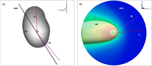
Figure 1. Schemes illustrating the orientation of the coordinate system, HP, HDP, Voyager trajectories, and the LISM velocity and magnetic field vectors. The views are (a) parallel to  and (b) perpendicular to the HDP.
Download figure:
Standard image High-resolution imageThe determination of the HDP plays a fundamental role in the recent analysis of the SW–LISM interaction, primarily because of its correlation with the IBEX measurements. According to McComas et al. (2009), the directions to the IBEX ribbon correlate with the directions perpendicular to the ISMF lines deformed by the HP in the simulation of Pogorelov et al. (2009b), where the B − V plane was parallel to the HDP. The simulation of Heerikhuisen et al. (2010) with the same choice of the B − V plane orientation reproduced the shape of the ribbon. Moreover, Heerikhuisen & Pogorelov (2011) showed that the ribbon readily responds to changes in the orientation of the B − V plane. Additionally, the choice of the ISMF vector in the HDP is favorable for the explanation of the energetic ion streaming directions observed by Voyager (Opher et al. 2006; Pogorelov et al. 2007). The direction of the LISM velocity is aligned with the vector  (Moebius et al. 2004). Here we choose a Cartesian coordinate system with the origin at the Sun, its x-axis being aligned with the Sun's rotation axis. The z-axis belongs to the plane determined by the x-axis and
  and is directed upwind into the LISM. The y-axis completes the right coordinate system. The HDP is defined by
  and the vector
  at which LISM neutrals enter the inner heliosphere (Lallement et al. 2005).
We use a one-fluid approximation for charged particles, i.e., the presence of PUIs, which are created in all regions of the heliosphere when neutral particles exchange charge with ions, is taken into account approximately assuming that PUIs, on average, quickly acquire the velocity of the ambient SW and that the effective temperature of the ion mixture is determined by the sum of the internal energies of PUIs and thermal core ions. The ion distribution is not necessarily Maxwellian, but can be an isotropic Lorentzian with κ = 1.63 (Heerikhuisen et al. 2008). This allows us to take into account high-energy tails in the plasma distribution, which are due to the presence of PUIs. As seen from the V2 observations (Richardson et al. 2008), PUIs are not in equilibrium with the core plasma.
3. THE SHAPE OF THE HELIOPAUSE, THE PRESSURE DISTRIBUTION ON IT, AND THE SURFACE 

3.1. Strong ISMF and the Validity of the Parker Solution
Before discussing the ISMF effect on the HP shape and on the topology of the surface where, according to McComas et al. (2009) and Heerikhuisen et al. (2010) charge exchange could create an enhanced flux of ENAs, we will summarize the behavior of the HP under the action of the increasingly large ISMF strength B∞ in an axially symmetric case. Such scenarios can be implemented if  and
and  in the SW. Parker (1961) considered two extremes of such interaction: (1) the expansion of the supersonic SW into a magnetized vacuum and (2) the interaction of the subsonic, nearly incompressible SW with the subsonic LISM carrying no substantial magnetic field. These classical solutions are very different: (1) results in the HP open in both upwind and downwind directions along the symmetry axis (squeezed laterally by a strong magnetic field, SW plasma can easily propagate along the magnetic field lines), while (2) creates an HP open only in the downwind direction with the SW streamlines diverted backward when they reach the HP. The latter case involves neither a TS nor a bow shock (BS). In the former case the Alfvén number A∞ = V∞/aA∞ is zero. To reproduce that solution numerically, it suffices to assume that A∞ < 1. If we introduce a closed tangential discontinuity separating SW from the LISM initially at t = 0, the HP quickly expands in both directions along the magnetic field lines, while it takes longer for it to propagate upwind. As seen from Figure 2 showing the plasma density distribution, ultimately the HP opens at any fixed radius of the circular outer boundary. The distances are given in AU throughout the paper. This solution is obtained in the ideal MHD formulation (no neutral particles) of the problem assuming B∞ = 6 μG, i.e., the LISM flow is sub-Alfvénic. For any chosen size of the outer boundary sphere t > 0 exists such that the HP is open in both upwind and downwind directions, in perfect agreement with the Parker scenario. It is known, however, that the LISM flow is supersonic. Thus, the described situation corresponds to a classical case of a superslow, but subfast, magnetosonic flow. This means a slow-mode BS is possible, but is not implemented because the HP travels to infinity upstream along the symmetry axis. The solution becomes qualitatively different if the interstellar neutral atoms are taken into account (Florinski et al. 2004). Charge exchange provides a drag, preventing the HP motion upwind. The HP finds its steady state, and a slow-mode shock is formed ahead it. We point out that this problem is of interest from the viewpoint of the MHD theory because the steady MHD equations have no characteristics in this case. This means that the BS cannot degenerate into a characteristic line far from the interaction region and must have a finite extent in space. Mathematically, this means that the Hugoniot shock relations have a slow-mode shock solution, but there is no solution to the linearized shock relations (Kogan 1959). This shock is seen in a four-fluid (one plasma and three neutral fluids; see Zank et al. 1996 for more details) simulation, where we choose nH∞ = 0.15 cm−3 and B∞ = 4 μG. Figure 3 clearly illustrates the bow shock behavior drastically differing from what usually happens in gas dynamics. Thus, one has to conclude that Parker's scenario (2) based on the assumption of a subsonic LISM may not be valid even in a strong magnetic field approximation because of the possibility of a slow-mode MHD shock.
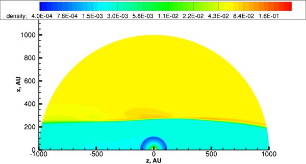
Figure 2. Axially symmetric SW–LISM interaction under strong ISMF conditions: in the absence of neutral particles the heliopause remains open at any distance from the Sun in the LISM upwind and downwind directions. The number density distribution is given in cm−3.
Download figure:
Standard image High-resolution image
Figure 3. Axially symmetric SW–LISM interaction for B∞ = 4 μG: thermal pressure distribution allows us to see a slow bow shock (the slow magnetosonic velocity coincides with the speed of sound) of finite vertical extent. In contrast with the situation shown in Figure 2, the presence of neutral particles allows the heliopause to find its stationary position at a finite heliocentric distance. The units are picodynes cm−2.
Download figure:
Standard image High-resolution imagePogorelov et al. (2006) considered the case of a strong ISMF (4 μG) in a three-dimensional formulation, assuming a small, 15° angle between  and
and  . In that simulation, the LISM velocity vector belonged to the meridional plane formed by
  and the Sun's rotation axis. Figure 4 shows the HP colored by the value of total (magnetic plus thermal) pressure in picodynes cm−2. We also show the ISMF lines starting in the unperturbed LISM and draping around the HP. Compressed by magnetic field, the HP is visibly elongated in the vertical direction (x-axis), extending over 500 AU above the ecliptic plane. The total pressure maximum shows up as a bright spot concentrated near the HP nose and is slightly shifted below the ecliptic plane. As seen from the two-dimensional, axially symmetric simulation of Florinski et al. (2004) and three-dimensional results presented above, Parker's scenario (1) is impossible in the presence of interstellar neutrals if we use reasonable values for B∞ and nH∞. Although they cannot sense the HP directly, interstellar neutrals start experiencing meaningful charge exchange with the LISM ions once they decrease their velocity interacting with the HP. Newly created atoms have low velocity and form a "hydrogen wall" on the external side of the HP (Wallis 1971, 1975; Baranov & Malama 1993; Pauls et al. 1995; Linsky & Wood 1996). Newly created ions have velocities of the parent atoms. They should be decelerated at the HP, and therefore exert additional pressure onto it. This additional pressure lets the HP acquire a stationary position in space. These considerations caution us against the application of the models (McComas et al. 2009; Krimigis et al. 2009; Gamayunov et al. 2010) based on the Parker solution, which turns out to be valid only in the absence of interstellar neutral atoms. Note that the observational estimates of Gloeckler et al. (1997) suggest that nH∞ can be three times as large as n∞.
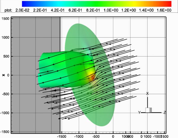
Figure 4. Distributions of the total pressure (in picodynes cm−2) on the surface of the heliopause and the surface  under strong ISMF conditions (B∞ = 4 μG). The vector
  is at 15° to the LISM velocity vector and belongs to the meridional (xz)-plane, nH∞ = 0.1 cm−3.
Download figure:
Standard image High-resolution imageIt is clear that the surface  degenerates into a plane
  far from the HP. This plane is perpendicular to
  and contains the origin of our coordinate system (the Sun). This means that ENAs created in the vicinity of the planar part of the
  surface will be observed by an observer looking in directions perpendicular to the ISMF direction in the unperturbed LISM. Figure 4 also reveals that the perturbation of the surface is located compactly near a very "slim" HP. The ribbon in this case should very likely be closer, compared with the lower magnetic field scenarios, to a full circle on IBEX sky maps. We also see that ideal MHD-neutral simulation does not show any narrow localized region of enhanced total pressure on the HP surface that could topologically be responsible for the ribbon, as was suggested in one of the possible scenarios discussed by McComas et al. (2009).
3.2. The Heliopause in Equilibrium: The Distribution of the Total Pressure
As mentioned in the previous section, Krimigis et al. (2009) and McComas et al. (2009) suggested that a narrow region of enhanced pressure on the HP surface, which is caused by the ISMF draping the HP, might create a sort of a three-dimensional flow separation line of enhanced plasma pressure and density in the IHS, and topologically resembles the observed ribbon. If correct, this line can be attributed to the region on the HP surface where  is close to zero. Here
  is the normal to the HP surface. Although the IBEX ribbon is subject to variations caused by the variability in the SW conditions (McComas et al. 2010), we will first analyze two steady-state solutions based on the simulations reported in Pogorelov et al. (2008, 2009b). They were obtained under the assumption that
  belongs to the HDP and is at 30° to
  . Two ISMF strengths were considered, B∞ = 3 μG (Case 1) and 4 μG (Case 2). Both cases reproduce the ribbon shape and predict ENA fluxes inside the ribbon reasonably well (Heerikhuisen et al. 2010). In Figure 5, we show the HP, the surface
  , and magnetic field lines for Case 2. Both surfaces are colored by the value of total pressure ptot = ptherm + pmag, which is the sum of the plasma thermal pressure and magnetic pressure (the units are pdyn cm−2). We are not talking here about the LISM ram pressure because at the surface of the HP the normal component of the velocity vector vanishes. As a result, the stress tensor on the surface separating SW from the LISM involves only the component
  depending on the LISM velocity (
 is the velocity component tangent to the HP). In stationary gas dynamics, the Bernoulli integral expresses the conservation of energy along streamlines. There is no analogue for the Bernoulli integral in ideal MHD (electric field
  ) unless the influx of the electromagnetic energy, proportional to
  , is parallel to the velocity vector
  . This condition is not satisfied either in the unperturbed LISM or in the OHS, unless
  (
( ) or
) or  . For this reason, electromagnetic energy is continuously flowing into (or out of) stream tubes. This makes it difficult to translate quantities from the unperturbed LISM to the HP surface without numerical solution of the MHD system for plasma with the source terms provided by the solution of the Boltzmann equation for neutral hydrogen, as done in this paper.

Figure 5. Distributions of the total pressure (in picodynes cm−2) on the surface of the heliopause and the surface  under strong ISMF conditions (B∞ = 4 μG): the vector
  is at 30° to the LISM velocity vector and belongs to the HDP, nH∞ = 0.15 cm−3.
Download figure:
Standard image High-resolution imageWe see that the surface  crosses the HP, which creates a whole in it. It is notable that the surface
  deviates from the planar shape considerably both in Case 1 and Case 2 (see Figure 6). However, this happens in a different way at distances far away from the HP (which do not contribute to the ribbon flux) and near it. For stronger
  , the deviation starts immediately near the outer boundary, since the absence of the BS allows fast magnetosonic perturbations to propagate upstream. The deformation of the
  surface by the HP starts closer to the intersection line between them. A systematic study of the ribbon behavior under the ISMF increase is presented by Heerikhuisen & Pogorelov (2011). They showed that the ribbon is likely to be created from ENAs born around the surface
  within a distance of about 100 AU from the HP. It is therefore understandable that the ribbon should become closer to a Sun-centered full circle as we increase
  . The approximation of the ribbon by an incomplete circle discussed by Funsten et al. (2009) reveals that this circle is not Sun-centered and very strong ISMF strengths are therefore unlikely. On this basis, our model tends to support conditions in the LISM where |B∞| < 3 μG. Heerikhuisen & Pogorelov (2011) also found that changes in the interstellar hydrogen density (the increase in nH∞ must be compensated by a corresponding decrease in n∞) result in only small changes in the shape and location of the ribbon produced by the simulation. Additionally, it was also found that we should have nH∞ ≈ 0.15 cm−3 in the LISM to have nH ≈ 0.09 cm−3 at the TS, as required to match observations of PUIs in the inner heliosphere (Gloeckler et al. 1997).
Here we consider Case 1 in more detail. Borovikov et al. (2011) used the set of parameters corresponding to this solution to compare the plasma distributions along the V1 and V2 trajectories, demonstrating a good agreement with the Voyager observations. Figure 6 shows the HP together with the surface  and the plane
  . We also show the ISMF lines draping around the HP, which causes the deviation between the latter two surfaces. One can easily see that they coincide only in a small region, which is quite far from the HP and likely does not contribute substantially to the ribbon flux. The reason for a strong deviation between the above-mentioned surface and plane is the subfast magnetosonic character of the LISM flow at B∞ = 3 μG.
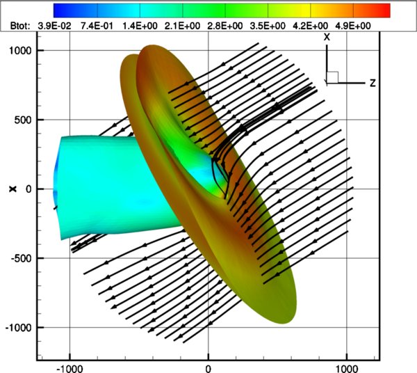
Figure 6. Heliopause, the surface  , and the plane
  for B∞ = 3 μG; the vector
  is at 30° to the LISM velocity vector and belongs to the HDP. The ISMF lines drape around the heliopause creating a spot of large magnetic field magnitude (given in μG) in the vicinity of the nose.
Download figure:
Standard image High-resolution imageThe balance of the total pressure on the SW and LISM sides of the HP ultimately determines its shape and location in space. Figure 7 shows the frontal view of the HP colored, from the left to the right, by the thermal, magnetic, and total pressure values. We see that in the framework of our MHD-kinetic model, where a non-isotropic distribution of PUIs in the vicinity of the TS is not taken into account, we observe a region of increased total pressure concentrated near the HP nose. Topologically, this region cannot be responsible for the observed shape of the ribbon. Since ptot is the same on the both sides of the HP, we conclude that the model does not show any crest in the total pressure distribution, which might create a flow separation zone. The reason for the presented behavior of the total pressure is the following. Because of the chosen orientation of  the maximum of the magnetic pressure is shifted southeast. As a result, the HP rotates exposing its northern hemisphere side to the LISM ram pressure that translates into ptherm on the HP surface, the maximum of which appears to be shifted northward. The maximum of the sum of the two pressures is therefore near the HP nose.
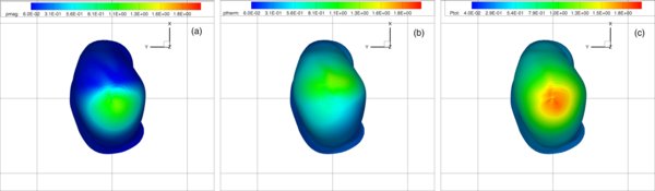
Figure 7. Frontal (interstellar) view of the HP colored by the values of (a) magnetic pressure, (b) thermal pressure, and (c) total pressure. The units are picodynes cm−2, the coordinate rectangle size in the plot is 500 × 500 AU.
Download figure:
Standard image High-resolution imageAs one would expect from the correlation of the ribbon directions with those of  , the choice of the ISMF strength and orientation determines the average shape of the ribbon. McComas et al. (2009), Schwadron et al. (2009), Heerikhuisen et al. (2010) showed that the choice of
  in the HDP at about 30° to
  results in an impressive agreement in the observed and simulated ribbon positions. Moreover, ENA fluxes computed by Heerikhuisen et al. (2010) for different energy bands reasonably agree with the observations within the ribbon. Heerikhuisen & Pogorelov (2011) have systematically investigated the effect of the ISMF strength and orientation on the ribbon position and found the range of optimum regimes. It was also shown that the choice of
  considerably off the HDP, as in Ratkiewicz & Grygorczuk (2008) and Opher et al. (2009), shifts the ribbon away from its observed position on the sky map (see also Pogorelov et al. 2010b). In this way, fitting the IBEX ribbon and satisfying the Lyα backscattered emission data together give us a powerful tool for remotely probing the LISM properties in the vicinity of the heliosphere.
4. SOLAR CYCLE AND IBEX MEASUREMENTS
The SW is variable on different timescales. Apart from numerous transient streams propagating from the Sun, we examine the solar rotation and solar cycle effects, with the characteristic scales of about 25 days and 11 years, respectively. It takes about six months for IBEX to create one full-sky map. It is interesting for this reason to analyze how the consequences of solar cycle are seen in the IBEX maps. On the other hand, the nature of the ENA flux is such that it takes 0.5–12 years for particles of different energy detectable by IBEX to reach the instrument from the site of their creation. In practice, this means that time-dependent simulations are critical for the efficient interpretation of the IBEX data. This is convincingly confirmed by the variations in the first two ENA maps (McComas et al. 2010). Sternal et al. (2008) pioneered modeling of the ENA flux dependence on the solar cycle and found that three-dimensional all-sky ENA flux maps are time varying due to the solar activity cycle. In our solar cycle model based on Pogorelov et al. (2009a), we qualitatively follow the average Ulysses observations (McComas et al. 2000), where during solar minimum the slow SW occupies heliolatitudes of approximately −35° ⩽ θ0min ⩽ 35°. The SW velocity, density, and temperature in slow wind at 1 AU are VEs = 4 × 107 cm s−1, nEs = 8 cm−3, and 105 K, respectively. The parameters in the fast SW are VEf = 8 × 107 cm s−1, nES = 3.6 cm−3, and 2.6 × 10⁵ K. The IMF radial component at 1 AU is 28 μG. The vector  in the SW is assumed to be given by Parker's formulae (Parker 1961) at the inner boundary. We also assume that the angle between the Sun's rotation and magnetic-dipole axes is initially α = αmin = 9°, and further changes periodically reaching maximum at 90° and changing polarity at solar maxima. Accordingly, the latitudinal extent of slow SW changes between its minimum value and 90° at solar maxima. In the solar cycle simulation, we adopt n∞ = 0.05 cm−3 and nH∞ = 0.15 cm−3. Here we use our time-dependent simulations of the solar cycle to analyze the variations in the shape of the
  surface and plasma density on it. Note the change in the coordinate axes' orientation compared with the results shown in the previous section. Now we exchange the x- and z-axis, and therefore changed the direction of the y-axis to the opposite. This choice better suits the calculation with varying latitudinal extent of slow SW and the tilt of the Sun's magnetic axis.
Figure 8 shows the evolution of plasma density in the meridional plane over almost a full solar cycle. Variation in the latitudinal extent of slow SW generates the regions of varying density in the IHS. In the framework of the physical scenario attributing the ribbon flux to ENAs born in the OHS, of importance are the variations in the plasma density detected by our numerical simulation in that region. Since the density changes can be as large as a factor of two, they can change the production rate of secondary neutral particles in the OHS. These neutrals create a hydrogen wall (Baranov & Malama 1993; Pauls et al. 1995; Zank et al. 1996) in front of the HP and participate directly in the creation of secondary ENAs possibly generating the ribbon due to a line-of-sight selection effect. Figure 9 shows that the above-mentioned behavior of plasma density can also be seen on the  surface. In these figures, this surface is shown at the same moments of time as in Figure 8 and colored by the plasma density. As shown in Heerikhuisen & Pogorelov (2011), most of the ribbon ENAs at energy of about 1 keV may be created in the vicinity of this surface at distances no more than 100 AU from the HP. The color and the orientation of the
  surface are such that one should expect an enhanced ENA flux in the southern part of the ribbon. One can see also substantial variations in the plasma density that are likely to cause variability in the ENA flux. It is worth noticing that the shape of this zone of larger plasma density is nearly circular and shifted in the direction indicated by the IBEX observations (see also Figure 10 for another perspective). There is a more variable zone in the northeast part of the
  surface. The latter appears to be narrow and propagating in the northwest direction away from the HP. One can speculate that this area may be partly responsible for the "knot" at the top of the ribbon (McComas et al. 2009, 2010). The deviation of the
  surface from the plane
  is important for producing a sufficiently broad ENA ribbon and ensuring its proper location in sky maps. Time variations in the normal to the
  are also of importance since they act to introduce a fine structure to the ribbon. More detailed analysis of these issues is outside the scope of this paper and will be addressed separately. To accurately reproduce observational ENA fluxes, we will require the development of a data-driven model of the heliosphere. Some preliminary results of the solar cycle simulations using Ulysses data are shown in Pogorelov et al. (2010a).
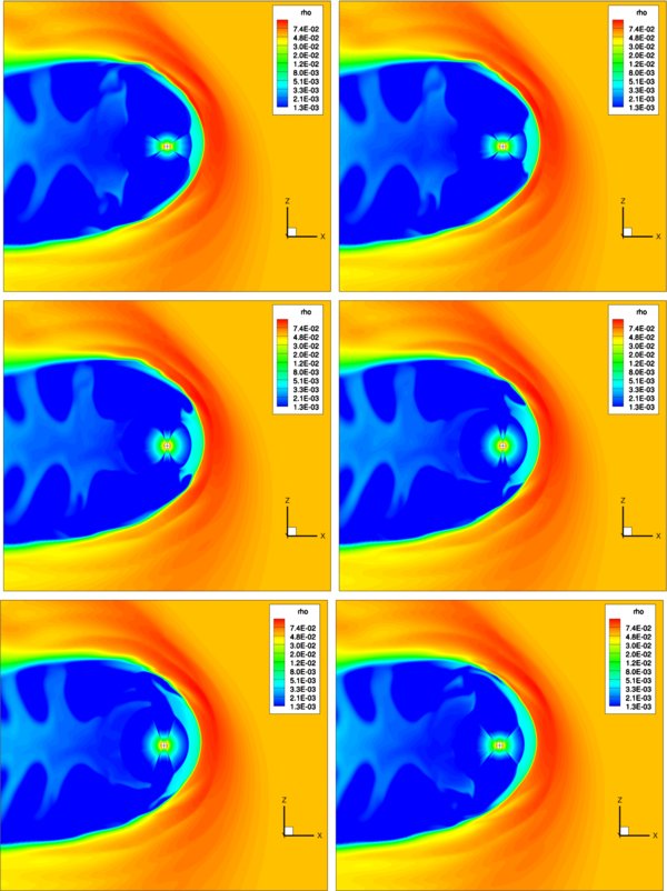
Figure 8. Variation of the plasma number density (in cm−3) within a solar cycle.
Download figure:
Standard image High-resolution image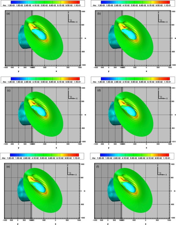
Figure 9. Evolution of the surface  and plasma density (in cm−3) on it over the solar cycle shown in Figure 8. The heliopause is shown with a blue color. Changes in the plasma density and in the normal to the surface should play an important role for the fine structure of the IBEX ribbon.
Download figure:
Standard image High-resolution image
Figure 10. Frontal (interstellar) view of the HP and the surface  . The surface is colored with the values of the plasma density (in cm−3).
Download figure:
Standard image High-resolution image
5. CONCLUSIONS
We have presented an analysis of the heliospheric response to changes in the strength and orientation of the ISMF. The B − V plane (the plane formed by the  and
and  vectors) was fixed according to the information of the neutral H velocity direction derived from the Lyα backscattered emission results in the Solar and Heliospheric Observatory Solar Wind Anisotropy experiment. This choice appears to be supported by the IBEX measurements of the ribbon—a thin layer of enhanced ENA flux spreading over the sky. The location of the ribbon strongly correlates with the directions where the ISMF vector is perpendicular to the line of sight in the simulations of Pogorelov et al. (2008, 2009c). Heerikhuisen et al. (2010) showed that this correlation can be explained by the mechanism of generating secondary ENAs in the OHS and quantitatively demonstrated its feasibility. Heerikhuisen et al. (2010) and Gamayunov et al. (2010) showed that the presence of a sufficient PUI pitch angle scattering in the OHS is essential for the reproduction of the ribbon flux which otherwise would be substantially overestimated. The concerns regarding the stability of the PUI distribution function raised by the one-dimensional simulations of Florinski et al. (2010) were partially addressed by Gamayunov et al. (2010) who modeled the evolution of the PUI distribution function and showed the importance of the energy cascading into the direction perpendicular to the OHS magnetic field. Their parametric studies of the mechanism described in McComas et al. (2009) and Heerikhuisen et al. (2010) show that the PUI distribution function behavior in the OHS may make the secondary ENA source of the ribbon tenable, although further investigation of the microscopic turbulence generated by PUIs will be necessary.
The analysis presented in this paper shows that (1) the Parker (1961) pattern of the SW expansion into the magnetized vacuum (all LISM Mach numbers are identically zero) is not valid even for a subfast LISM flow in the presence of charge exchange between the interstellar ions and neutrals at the front side of the HP (see also Florinski et al. 2004; Pogorelov et al. 2006); (2) the distribution of total pressure on the surface of the HP due to its draping by the ISMF exhibits a broad localized increase in the nose area where the deformation of ISMF lines is maximal; (3) our SW–LISM model with the effect of PUIs taken into account by assuming an isotropic Lorentzian (kappa) distribution of ions in the OHS (Heerikhuisen et al. 2008) does not demonstrate any spatially narrow increase in the total pressure on the HP surface that, after being translated to its inner side, may create a plasma flow division line topologically resembling the ribbon; (4) the increase of  above 3 μG deforms the HP and the
  surface in a way not consistent with the IBEX ribbon as it was observed (this is also confirmed by the direct simulation of the ribbon ENA fluxes by Heerikhuisen & Pogorelov 2011); (5) the solar cycle affects the surface
  in the OHS at timescales that can be resolved by the IBEX detectors creating a full all-sky map approximately every six months; (6) a region of enhanced LISM plasma density located in the southern part of the interaction region persists over the solar cycle and may be responsible for the corresponding enhancement of the ENA flux observed by IBEX; the spectral index of the flux should therefore depend on time as the primary ENAs propagate at these latitudes with different velocities depending on the latitudinal extent of slow wind; and (7) a much more localized and variable region of enhanced plasma density exists in the northern part of the HP intersection with the
  surface (note that according to Heerikhuisen et al. 2010 and Heerikhuisen & Pogorelov 2011 the ribbon flux is mostly created at distances of about 100 AU from the HP into the OHS), which may be responsible for the knot in the corresponding region of the ribbon.
Although there are many studies supportive of the OHS scenario of the ribbon, one cannot exclude the possibility of other mechanisms. According to the analysis presented in this paper, such alternative mechanisms should necessarily involve some kind of an anisotropic distribution of PUIs—the scenario also outlined in McComas et al. (2009). Such a distribution can be created at the TS (see, e.g., Zank et al. 2010; Kucharek et al. 2010). So far there is no direct quantitative analysis of this process.
This work is supported by NASA grants NNX08AJ21G, NNX08AE41G, NNX09AW44G, NNH09AG62G, NNH09AM47I, NNX09AP74A, NNX09AG63G, NNX10AE46G, and the UAHuntsville Research Infrastructure Investment grant. Supercomputer time allocations were provided on SGI Pleiades by NASA High-End Computing Program award SMD-10-1691, Cray XT5 Kraken by NSF Teragrid project MCA07S033, and on Cray XT5 Jaguar by ORNL Director Discretion project PSS0003. This work was also partially supported by the IBEX mission as a part of NASA's Explorer program.