


ABSTRACT
In this study, a novel ab initio cosmic ray (CR) modulation code that solves a set of stochastic transport equations equivalent to the Parker transport equation, and that uses output from a turbulence transport code as input for the diffusion tensor, is introduced. This code is benchmarked with a previous approach to ab initio modulation. The sensitivity of computed galactic CR proton spectra at Earth to assumptions made as to the low-wavenumber behavior of the two-dimensional (2D) turbulence power spectrum is investigated using perpendicular mean free path expressions derived from two different scattering theories. Constraints on the low-wavenumber behavior of the 2D power spectrum are inferred from the qualitative comparison of computed CR spectra with spacecraft observations at Earth. Another key difference from previous studies is that observed and inferred CR intensity spectra at 73 AU are used as boundary spectra instead of the usual local interstellar spectrum. Furthermore, the results presented here provide a tentative explanation as to the reason behind the unusually high galactic proton intensity spectra observed in 2009 during the recent unusual solar minimum.
Export citation and abstract BibTeX RIS
1. INTRODUCTION
Although not new (see, e.g., Jokipii & Owens 1975; Jokipii & Levy 1977), the stochastic approach to solving the Parker (1965) transport equation (TPE) in cosmic ray (CR) modulation studies has recently become quite popular (see, e.g., Zhang 1999; Alanko-Huotari et al. 2007; Pei et al. 2010; Strauss et al. 2011; Della Torre et al. 2012; Luo et al. 2013). This is due to a number of factors. First, this approach allows one to solve the three-dimensional (3D), energy-, and time-dependent Parker TPE without the perceived disadvantages implied by the use of a numerical grid, implicit to more traditional finite-difference schemes such as the alternating direction implicit (ADI) scheme (see, e.g., Peaceman & Rachford 1955). Second, this approach readily lends itself to parallel computing techniques. Computer clusters are becoming less expensive and more powerfeul, making computationally expensive techniques such as this ever more feasible. Lastly, and perhaps most importantly, this approach is not plagued by the numerical stability issues that so often limit studies of CR modulation using finite-difference techniques. With these considerations as motivation, a stochastic technique is here applied to the study of CR modulation in an ab initio approach. This entails treating the turbulence power spectra as the basic inputs for the modulation study, using diffusion coefficients derived from these spectra with recent, novel scattering theories, and modeling the spatial dependence of the various basic turbulence quantities throughout the heliosphere with a turbulence transport model (TTM) that yields results in reasonable agreement with spacecraft observations of the same.
This paper is organized as follows. A detailed introduction to the numerical technique followed in this approach, as well as other details pertaining to such a CR modulation code, is given in Section 2. The code presented in this study incorporates several refinements and recent advances in scattering theory not taken into account in previous studies. It is benchmarked against the results of Engelbrecht & Burger (2013a) in Section 2.1. A novel aspect of the current approach is the use of CR boundary intensity spectra constructed using Voyager observations within the heliospheric termination shock as input for the stochastic modulation code, discussed in Section 2.2. This is motivated by the fact that previous ab initio codes, due to assumptions implicit to the TTMs they used, could not take into account the effects of the heliosheath, a region where a considerable amount of CR modulation occurs. The new input intensity spectra provide a way to take this modulation into account without necessitating ad hoc assumptions as to particle and turbulence transport in the heliosheath. Their use also allows for the testing of assumptions as to the transport coefficients employed on CR intensities computed from first principles, when these intensities are compared to spacecraft observations at Earth. Results from the Oughton et al. (2011) two-component TTM are used as inputs for an observationally and theoretically motivated form of the two-dimensional (2D) turbulence power spectrum. New perpendicular mean free path expressions derived using this spectral form from the unified nonlinear theory (UNLT) of Shalchi (2010) as well as those derived by Engelbrecht & Burger (2013b) from the extended nonlinear guiding center (ENLGC) theory of Shalchi (2006) are employed. This spectral form is also used to derive an expression for the 2D ultrascale (see, e.g., Matthaeus et al. 2007), which is a key input for the turbulence-reduced drift coefficient of Burger & Visser (2010) used in this study. These transport parameters are discussed in Section 3. The diffusion and drift coefficients have been shown by Engelbrecht & Burger (2014) to be extremely sensitive to assumptions made regarding the low-wavenumber behavior of the 2D turbulence power spectrum, albeit using a different 2D spectral form and different turbulence quantities in their calculations with a finite-difference ab initio modulation code. Taking this into account, various values and spatial scalings for the 2D outerscale, the lengthscale at which energy-containing range on the assumed 2D turbulence power spectrum commences, are chosen based on what little is currently known of this quantity. The differences between the abovementioned ENLGC and UNLT perpendicular mean free path expressions as a function of these assumed forms for the 2D outerscale are investigated at various rigidities and as a function of heliocentric radial distance in Section 4. The Burger & Visser (2010) turbulence-reduced drift coefficient is also sensitive to the behavior of the 2D outerscale, and is similarly studied. Finally, galactic proton CR intensities at 1 AU computed assuming these various forms of the 2D outerscale, for perpendicular mean free path expressions derived from both scattering theories considered here, are presented in Section 5, and compared with spacecraft observations. Conclusions drawn as to the possible low-wavenumber behavior of the 2D turbulence power spectra at large radial distances are presented in Section 6.
2. THE MODULATION MODEL
The Parker CR transport equation in the absence of sinks and sources of energetic particles is given by
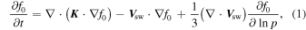
with f0( , p, t) the omnidirectional CR phase space density, as a function of particle momentum p, and related to the observationally reported CR differential intensity by jT = p2f0 (see, e.g., Moraal 2013). Various processes modulating an initial interstellar CR differential intensity jLIS are contained within the above equation, including CR diffusion, drift due to gradients in and curvatures of the heliospheric magnetic field (HMF), the effects of the outward convection of CRs by the solar wind, and adiabatic cooling.
Following the approach outlined by Zhang (1999), Pei et al. (2010), and Strauss et al. (2011), Equation (1) can be written in terms of a set of equivalent Itō stochastic differential equations (SDEs) given by

with ![$i\in [r,\theta ,\phi ,E],$](https://content.cld.iop.org/journals/0004-637X/814/2/152/revision1/apj521505ieqn2.gif) and xi(t) Ito processes (see, e.g., Zhang 1999; Gardiner 2004). Furthermore, dWi satisfy a Weiner process, such that (Pei et al. 2010; Strauss et al. 2011)
and xi(t) Ito processes (see, e.g., Zhang 1999; Gardiner 2004). Furthermore, dWi satisfy a Weiner process, such that (Pei et al. 2010; Strauss et al. 2011)

where η(t) represents a pseudo-random, Gaussian-distributed number between zero and one. Pseudo-random numbers are generated in this study following the same approach as that of Strauss et al. (2011), by using the Mersenne Twister algorithm developed by Matsumoto & Nishimura (1998).
In the present study, Equation (2) is solved in the time-backward manner using the Euler–Maruyama approximation (Maruyama 1955) employed by, e.g., Pei et al. (2010) and Strauss et al. (2011), so that the evolution of a large number N of pseudo-particles with a particular energy at an initial specified phase space point and time  is iteratively followed to their exit points and times (and energies)
  at some specified boundary, after which the average CR intensity at the initial point is calculated with (Strauss et al. 2011)

using the assumed intensity at the boundary jLIS. Assuming a generalized three-component HMF, Pei et al. (2010) show that
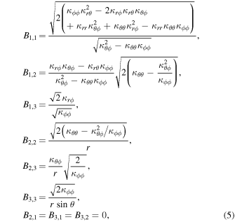
whereas the components of the vector  are given as
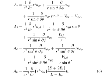
The quantity Eo is the rest-mass energy of the species of CR in question, and κi,j denote elements of the diffusion tensor  in Equation (1). Note that the signs of the solar wind and drift speeds Vsw and Vd, as well as of AE, are the opposite of those presented in, e.g., Pei et al. (2010). This is to make it explicit that a time-backward approach is taken here in the solution of Equation (2). The components of the drift velocity are, as in Engelbrecht & Burger (2013a), calculated following the approach of Burger (2012). This allows for the calculation of the current sheet drift effects for large heliospheric tilt angles, even though the emphasis of the current study is on the modulation of galactic CR protons during solar minimum conditions.
The elements of the diffusion tensor are transformed in this model to a right-handed coordinate system aligned with a general 3D HMF using (Burger et al. 2008)
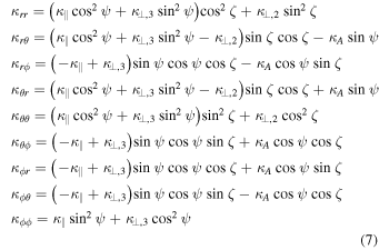
with the HMF winding angle denoted by ψ, and the angle ζ defined as
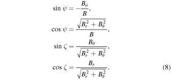
This means that the tangent of the HMF winding angle ψ becomes

which reduces to the usual definition of Bϕ/Br in a Parker (1958) HMF without a meridional component. The parallel, perpendicular, and antisymmetric diffusion coefficients given in Equation (7) will be discussed in more detail in Section 3. Note that in this study κ⊥,2 = κ⊥,3, as axisymmetric perpendicular diffusion is assumed. These diffusion and drift coefficients are extremely sensitive to assumptions made as to the behavior of the turbulence power spectra throughout the heliosphere (see, e.g., Shalchi et al. 2010; Engelbrecht & Burger 2013b), and require as inputs values for turbulence quantities such as the magnetic variance. These turbulence quantities are calculated here using the two-component Oughton et al. (2011) TTM. This model is solved as described by Engelbrecht & Burger (2013b) for generic solar minimum conditions, utilizing the same boundary values, and modeling turbulence-related terms in exactly the same way. The boundary values are chosen to yield model results in reasonable agreement with spacecraft observations of turbulence quantities throughout the heliosphere, as described by Engelbrecht & Burger (2013a). In the solution of this TTM, the pickup ion contribution to the wavelike fluctuations is ignored, as is done by Engelbrecht & Burger (2013b). This is due to the fact that the ionization of neutral hydrogen generates fluctuations at or near the wavenumber corresponding to the proton gyrofrequency (see, e.g., Isenberg et al. 2003; Isenberg 2005, and Cannon et al. 2014a, 2014b), close to the high-wavenumber dissipation range on the turbulence power spectrum (see, e.g., Leamon et al. 2000). Therefore, its contribution is not expected to significantly affect the level or wavenumber dependence of the fluctuation spectra at low wavenumbers, and hence not to significantly affect the transport for galactic cosmic ray protons with rigidities in the range (∼0.1–10 GV) of interest to this study. The Parker (1958) model for the HMF is employed, although by Equations (5) and (6) the modulation model presented here would also be able to deal with more complicated Fisk-type (Fisk 1996) HMF models, such as the Schwadron–Parker hybrid HMF proposed by Hitge & Burger (2010). The aim here is to model generic solar minimum conditions, and to this end the latitudinal solar wind speed profile is modeled using a hyperbolic tangent function, so that Vsw = 400 km s−1 in the ecliptic plane, and 800 km s−1 over the poles, as observed by Ulysses (McComas et al. 2000). Drift along the heliospheric current sheet is modeled following the approach of Burger (2012), assuming a tilt angle of 10°. This approach yields results in good agreement with the approach followed by Pei et al. (2010) and Strauss et al. (2012). These large-scale quantities simultaneously serve as inputs for the TTM and the SDE modulation code.
Use of the results of the Oughton et al. (2011) TTM as inputs for expressions for turbulence power spectra leads to complex spatial dependences for diffusion coefficients. To illustrate the origin of this dependence, contour plots of meridional slices taken at 0° azimuth of the variances and correlation scales, calculated from the results of the Oughton et al. (2011) TTM, are shown in Figures 1 and 2, respectively. For any given radial spoke, the variances shown in Figure 1 decrease almost monotonically with increasing radial distance due to the omission of pickup ion effects, a result consistent with the theoretical findings of Hunana & Zank (2010). Both variances tend to be larger toward the poles in the inner heliosphere, reflecting the observations of higher levels of turbulence at these latitudes reported by Forsyth et al. (1994), Bavassono et al. (2000a, 2000b), and Erdös & Balogh (2005), with slab variances becoming larger than 2D variances. Larger variance values at intermediate latitudes are due to increased stream-shear effects in the region where the slow solar wind transitions into the fast as a function of latitude.
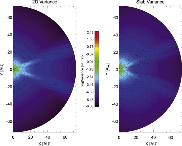
Figure 1. Slab (right panel) and 2D (left panel) variances calculated from the results of the Oughton et al. (2011) TTM, following the approach outlined by Engelbrecht & Burger (2013b).
Download figure:
Standard image High-resolution imageThe corresponding correlation scales are shown in Figure 2. Both scales broadly exhibit a latitudinal variation, with larger values toward the poles than in the ecliptic, in qualitative agreement with the observations reported by Dasso et al. (2005) and Weygand et al. (2011), with larger values for both quantities at latitudes corresponding to enhanced stream-shear effects. As a function of radial distance, the 2D correlation scale increases monotonically, also in qualitative agreement with the Voyager observations reported by Smith et al. (2001).
Figure 2. Correlation scales calculated from the results of the Oughton et al. (2011) TTM, following the approach outlined by Engelbrecht & Burger (2013b).
Download figure:
Standard image High-resolution image2.1. Benchmarking the SDE Model
As a benchmark of this newly developed model, comparisons are made with the results of Engelbrecht & Burger (2013a) using identical input parameters. Figure 3 shows a comparison of results for positive and negative magnetic polarity cycles (red lines for the ADI code and blue lines with squares for the stochastic code) as well as for the scenario where drift effects are neglected (thick black line for the ADI code and thin black line with squares for the stochastic code). Selected spacecraft observations are indicated by dots (McDonald et al. 1992) and triangles (Shikaze et al. 2007), respectively. The spacecraft data are shown simply to guide the eye. Clearly, for both magnetic polarity cycles, as well as for the no-drift scenario, the SDE approach yealds results in good agreement with those computed using the fully ab initio ADI modulation code of Engelbrecht & Burger (2013a). The maximum difference in results computed with these codes is less than 10%. Note, however, that intensities computed with the ADI code tend to decrease somewhat as magnitude of the momentum steps used is decreased. This would improve agreement between the approaches.
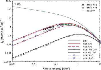
Figure 3. Galactic cosmic ray proton differential intensities calculated using the ADI ab initio modulation code of Engelbrecht & Burger (2013a; red lines) and the SDE approach employed here (blue lines and squares), for positive (solid lines) and negative (dashed lines) magnetic polarity cycles. Black lines and squares correspond to solutions where drift effects are switched off. Data shown are taken from McDonald et al. (1992) and Shikaze et al. (2007).
Download figure:
Standard image High-resolution image2.2. New Input Spectra
It has long been known that considerable CR modulation occurs within the heliosheath (e.g., McDonald et al. 2000; Caballero-Lopez et al. 2010), and recent Voyager observations reported by, e.g., Webber & McDonald (2013) and Stone et al. (2013) confirm this fact. Figure 4 shows the Burger et al. (2008) input spectrum as a function of energy, as well as Voyager observations of proton intensities at 122 AU reported by Stone et al. (2013; squares). This input spectrum, if used as a "local interstellar spectrum" at 100 AU as was done by Engelbrecht & Burger (2013a) at 100 AU, is clearly an overestimate. Furthermore, the heliospheric structure is much more complicated than previously assumed (see, e.g., Opher et al. 2015), so the assumption of a spherically symmetric heliosphere without a termination shock as made by Engelbrecht & Burger (2013a) is most likely an oversimplification. These assumptions, however, are necessitated by the fact that the Oughton et al. (2011) TTM is derived using assumptions that are not valid in the heliosheath. To circumvent this issue, an observationally motivated input spectrum is proposed here, based on galactic CR proton intensities observed by Voyager 1 and 2 before their termination shock crossings. Such a spectrum would already be modulated by whatever processes occur in the heliosheath, and would provide a more realistic input which can form the basis of comparisons of computed galactic proton intensities with spacecraft observations of the same in the inner heliosphere.

Figure 4. Galactic cosmic ray proton differential intensities observed by various spacecraft in different regions of the heliosphere, as well as the modulation code input spectra of Burger et al. (2008) and this study (black, red, and blue solid lines), as a function of kinetic energy. Squares denote Voyager 1 observations at 122 AU reported by Stone et al. (2013), and triangles Voyager 1 observations at 73 AU reported by Webber et al. (2008), while the black and white circles and the green stars represent 1 AU IMP8 and BESS97 observations taken from McDonald et al. (1992) and Shikaze et al. (2007).
Download figure:
Standard image High-resolution imageWebber et al. (2008) report on galactic proton intensities measured by both Voyager spacecraft prior to their respective termination shock encounters. These authors find a clear charge-sign dependence, with intensities detected by Voyager 2 during the negative polarity cycle (A < 0) being 1.4–1.7 times larger than those detected by Voyager 1 at 73 AU during the positive polarity cycle. The Voyager 1 intensities, taken at 73 AU, are shown in Figure 4 (red triangles), along with the same data, multiplied by a factor of 1.4 (blue triangles). The latter set of points will be taken to represent a lower estimate of the A < 0 intensities at 73 AU. Observations of proton intensities of Earth shown in Figure 3 are shown once more to guide the eye. To take into account the charge-sign dependence of the observations at 73 AU, two different input spectra were fit to Voyager observations. These fits (in units of particles per MeV per m2 per s per sr), based on the Burger et al. (2008) expression, are shown in Figure 4 (red and blue lines), and are given by

where P denotes the particle rigidity in GV, Po = 1 GV, and
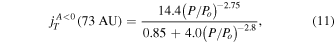
respectively. Note that these input spectra do not take into account anomalous protons, and therefore do not increase at the lowest energies (see, e.g., Fichtner 2001). The crossover of the new input spectra, seen at ∼0.025 GeV, occurs at an energy too low to affect the modulated intensity spectra to be presented here. In what follows, Equations (10) and (11) are used as boundary spectra in the ab initio SDE code at 73 AU, for the relevant magnetic polarity cycles.
3. THE DIFFUSION TENSOR
The diffusion coefficients parallel and perpendicular to the HMF κ∥ and κ⊥ in Equation (7) are related to the corresponding parallel and perpendicular mean free paths by κ∥,⊥ = (v/3)λ∥,⊥, with v the particle speed. In this study, a composite slab/2D model for turbulence is assumed (see, e.g., Bieber et al. 1994). The galactic proton parallel mean free path employed in this study is that used by, e.g., Burger et al. (2008) and Engelbrecht & Burger (2013a), based on the results derived from the quasilinear theory of Jokipii (1966) by Teufel & Schlickeiser (2003) for a slab turbulence power spectrum with a wavenumber-independent energy range, and an inertial range with a spectral index of −s. This expression is given by

where R = RLkmin is a function of the maximal Larmor radius RL and the wavenumber kmin at which the inertial range on the slab turbulence power spectrum commences. Note that Bo and  denote the uniform background HMF and the slab variance, respectively.
The perpendicular mean free path used by Engelbrecht & Burger (2013b) is used in this study. This expression is derived from the ENLGC theory of Shalchi (2006), which is based on the NLGC theory proposed by Matthaeus et al. (2003), and yields results in good agreement with numerical test simulations of the perpendicular diffusion coefficient as well as with spacecraft observations of the same (see, e.g., Shalchi 2006, 2009; Minnie et al. 2007a). From this theory, the perpendicular diffusion coefficient can be calculated, assuming magnetostatic axisymmetric perpendicular fluctuations,

where S2D denotes the 2D modal spectrum. Note that the modal spectrum is related to the omnidirectional spectrum by 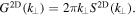 Equation (13) is similar to the NLGC expression given by Shalchi et al. (2004), but without the direct contribution from the slab spectrum. This omission is motivated by the fact that the numerical simulations of, e.g., Qin et al. (2002) show that the slab contribution is subdiffusive (Shalchi 2006, 2010, 2015). Note that the quantity a is a numerical constant, assumed here to have a value of
  after Matthaeus et al. (2003).
A new perpendicular mean free path expression, derived from the UNLT proposed by Shalchi (2010), is also employed in this study. In this theory, the perpendicular diffusion coefficient for slab/2D composite turbulence can be calculated using

Note that Equation (14) differs from the ENLGC result by only a factor of 4/3 in the denominator of the integrand. Perpendicular mean free paths for these models are derived here for a 2D turbulence modal power spectrum that yields a  wavenumber dependence in the energy-containing range of the omnidirectional power spectrum, given by Engelbrecht & Burger (2013b) as
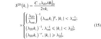
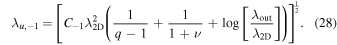
where the normalization constant C−1 is determined using  =
=  (see, e.g., Matthaeus et al. 2007), with
  the 2D variance. The normalization constant for this spectral form is given by Engelbrecht & Burger (2013b)

The form of this spectrum is motivated by spacecraft observations of turbulence at Earth (e.g., Bieber et al. 1993; Smith et al. 2006b). The quantity q represents the spectral index of an "outer" range at small wavenumbers added to this spectral form to ensure a finite 2D ultrascale (Matthaeus et al. 2007), a quantity employed in the following, and is set to a value of 3 based on physical considerations discussed by Matthaeus et al. (2007). The spectral index in the inertial range of this spectrum ν is set here at a Kolmogorov value of 5/3. Lastly, λout and λ2D are the length scales at which the energy-containing and inertial ranges commence. The perpendicular mean free path derived using this spectrum is given in a general form by
where the subscript E/U denotes the theory (either ENLGC or UNLT) used in the derivation of the mean free path.
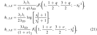
When the UNLT of Shalchi (2010) is used to derive λ⊥
where


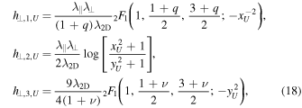
Using the ENLGC theory of Shalchi (2006) for a k−1 energy range, Engelbrecht & Burger (2013b) find that
where


The above expressions for the perpendicular mean free path are evaluated numerically. Following the approach of Engelbrecht & Burger (2013b), only the second terms of Equations (21) and (18) are evaluated, as the other terms contribute little to the final value of λ⊥ (see also Shalchi 2013, 2014).
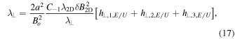
Drift coefficients (κA) are modeled to take into account the effects of turbulence (see, e.g., Jokipii 1993; Giacalone et al. 1999; Minnie et al. 2007b), following variously the approaches of Bieber & Matthaeus (1997), Burger & Visser (2010), and Tautz & Shalchi (2012). For the purposes of this study, only that proposed by Burger & Visser (2010) will be employed. This turbulence-reduced drift coefficient, which is a parametrization of the results proposed by Bieber & Matthaeus (1997) to agree with the numerical simulation results of Minnie et al. (2007b), is given by

where 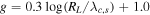 and λc,s is the slab correlation scale, is also sensitive to assumptions made as to the low-wavenumber behavior of the 2D turbulence power spectrum, as it is a function of the perpendicular field line random walk diffusion coefficient D⊥. This quantity, given by (Matthaeus et al. 1995), such that

where

and

which is a function of the 2D ultrascale, calculated by Engelbrecht & Burger (2013b) for the same spectral form as is assumed in this study as
In the following, the simplifying assumption is made that the 2D turnover scale is equal to the 2D correlation scale.
4. THE SENSITIVITY OF DIFFUSION AND DRIFT COEFFICIENTS TO CHANGES IN THE LOW-WAVENUMBER BEHAVIOR OF THE 2D TURBULENCE POWER SPECTRUM
In the present study, all turbulence quantities in Equation (15) except those pertaining to the "outer" range at the smallest wavenumbers are either modeled using the Oughton et al. (2011) TTM (as is the case for variances and correlation scales) or pre-specified based on spacecraft observations at Earth (as is the case for the spectral indices in the inertial and energy-containing ranges). This leaves only the 2D outerscale λout and the spectral index q of the outer range as candidates for a parameter study as to the effects of the low-wavenumber behavior of the spectrum on CR modulation. Of these quantities, the latter has been shown not to have a great effect on CR spectra computed with an ab initio modulation code (Engelbrecht 2013), while the former has been demonstrated to have a significant effect (Engelbrecht & Burger 2014), albeit with different diffusion coefficients and turbulence quantities. No spacecraft observations currently exist for either of these quantities, thus a relatively ad hoc scaling for the 2D outerscale must be chosen. This choice, however, can be guided to some degree by inferences drawn from extant observations of turbulence spectra at Earth, and from models of the transport of turbulent fluctuations throughout the heliosphere that can reproduce spacecraft observations, at least qualitatively, in the outer reaches of the heliosphere. The consensus from the latter appears to be that some form of driving still occurs at small wavenumbers even at great radial distances in the heliosphere, at least within the termination shock (see, e.g., Zank et al. 1996; Breech et al. 2008; Oughton et al. 2011 and Zank et al. 2012). This motivates the assumption, implicit to the fixed form chosen for the 2D spectrum in Equation (15), of an energy-containing range of finite extent at all radial distances considered, and therefore of a 2D outerscale consistently greater than the 2D turnover scale λ2D. Furthermore, observations of turbulence spectra at 1 AU have long resolved the energy-containing range, to the extent of one to two orders of magnitude in wavenumber, and yet do not find evidence of the outer range. This difficulty is probably due to the fact that at such large scales non-turbulent effects due to, e.g., solar rotation, begin to impinge on observations (Goldstein & Roberts 1999).
A choice, then, of a form for the 2D outerscale would then have it be at least two orders of magnitude larger than the 2D turnover scale at Earth. Motivated by these considerations, two simple forms for this quantity are chosen in such a way so that the effects of changes in its magnitude can most readily be discussed. The first approach assumes that λout would have the same radial dependence as the 2D correlation scale, but remain larger than it by a constant factor,

where λc,2D(r) is the 2D correlation scale yielded by the Oughton et al. (2011) TTM, and n is a constant taken to assume values of 10, 100, and 1000. The case where n = 1000 leads to a value for λout at 73 AU of 69.7 AU is included as a potential upper value for this quantity. To take into account the fact that the 2D outerscale needs to be at least two orders of magnitude larger than the 2D turnover scale (at least at Earth) as well as to consider an alternate radial dependence for this quantity, an alternative scaling is also employed, so that

with n chosen to be 100 and 1000, so that the outerscale in this case is constant. The value at Earth is that reported by Weygand et al. (2011), who find that λc,2D = 0.0074 ± 0.0007 AU. The results of the TTM employed here agree with this Weygand et al. (2011) value at 1 AU. The various forms of the 2D outerscale discussed above, along with the slab and 2D correlation scales yielded by the Oughton et al. (2011) TTM, are shown in the top panel of Figure 5 as a function of heliocentric radial distance in the ecliptic up to 73 AU, the extent of the model heliosphere in the SDE modulation code. While the case where λout = 10λc,2D (1 AU) is shown in this figure to illustrate that because it becomes roughly equal to λc,2D, this case leads to a scenario where no energy-containing range exists in the outer heliosphere, and is thus not considered here. All other 2D outerscales shown remain above λc,2D, and reach similar values at larger radial distances. Note that at 1 and 73 AU the outerscales for both scaling choices are equal at the former distance and very similar in value at the latter distance for the cases where n = 100 or n = 1000 in Equation (29) and n = 10 or n = 100 in Equation (30), respectively.
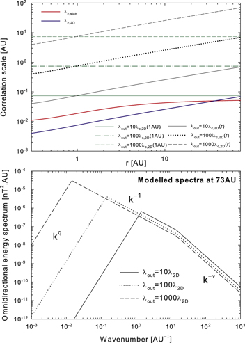
Figure 5. Top panel shows the assumed radial dependences for the 2D outerscales used in this study, along with the composite 2D and slab correlation scales yielded by the Oughton et al. (2011) TTM, also employed in this study. Bottom panel shows the modeled 2D omnidirectional power spectra G2D(k⊥) used in this study (see Equation (15) and the text below) for some of the assumed 2D outerscale values from the top panel, at 73 AU in the solar ecliptic plane. The turbulence quantities used to plot these spectra are taken from the Oughton et al. (2011) TTM. Note that only the 2D outerscale is varied from spectrum to spectrum, and that in this figure, as in the rest of the study, q = 3 and ν = 5/3.
Download figure:
Standard image High-resolution imageThe bottom panel of Figure 5 shows the modeled 2D omnidirectional spectra at 73 AU corresponding to the choices of 2D outerscale described by Equation (29), calculated with Equation (15) using outputs from the Oughton et al. (2011) TTM. Spectra calculated for outerscales scaling as Equation (30) are not shown, as these are indistinguishable from those in the figure due to the similarity in outerscales yielded by both scalings at this radial distance. As all three spectra are calculated assuming the same variance and turnover scale values, as well as using the same spectral indices for all three ranges, the net effect of modifying the 2D outerscale does not only affect to the extent of the energy-containing range in terms of wavenumber, but also the level of the spectrum. Therefore, larger values of λout lead to lower levels of the spectra, at least where their energy and inertial ranges overlap.
The parallel mean free path as well as the UNLT and ENLGC perpendicular mean free paths are shown as a function of rigidity in the ecliptic plane at 1 and 73 AU (top left and right panels) and as a function of heliocentric radial distance in the solar ecliptic plane for a rigidity of 1.5 GV (bottom panels) in Figure 6, for the various choices of 2D outerscale discussed above. Palmer (1982) consensus values are also shown at Earth. Only the choices of λout as defined by Equation (29) are shown in the top panels, as the scaling for this quantity defined by Equation (30) yields identical, or very similar, values for λout at the radial distances considered. This is not the case for the bottom panels, where both scalings are shown in their own panels to illustrate the effect of the different radial dependences of λout. Figure 7 is in the same format, showing the length-scale λA associated with κA as a function of rigidity and radial distance for the various choices of λout considered here. Note that the parallel mean free path remains unaffected by changes in λout, as this quantity has no bearing on the slab fluctuation spectrum used to derive λ∥. The parallel mean free path remains well above the Palmer consensus range for the rigidities shown here, due to the choice of boundary values for the TTM, to acquire solar minimum values for the various turbulence quantities of Equation (12) is a function (see, e.g., Engelbrecht & Burger 2013a). Considering both figures broadly, the results presented here differ considerably from those presented by Engelbrecht & Burger (2014), who also considered the effects of λout on the perpendicular mean free path and drift scale. This is due to two reasons. First, the 2D spectral form used here is different to that employed by Engelbrecht & Burger (2014), who assumed a flat energy-containing range. Second, Engelbrecht & Burger (2014) use outputs from the Oughton et al. (2011) TTM which include the pickup ion contribution to the wavelike fluctuation energy beyond ∼10 AU. These effects are neglected here, resulting in significant differences in the turbulence-related inputs between the two studies, especially at larger radial distances. The perpendicular mean free paths presented here, for instance, do not display the ∼P2 rigidity dependence reported by Engelbrecht & Burger (2014) below ∼1 GV at large radial distances simply because of the differences in the turbulence quantities employed. Qualitatively, however, from both studies it is clear that a large value of λout leads to a larger value for λ⊥.
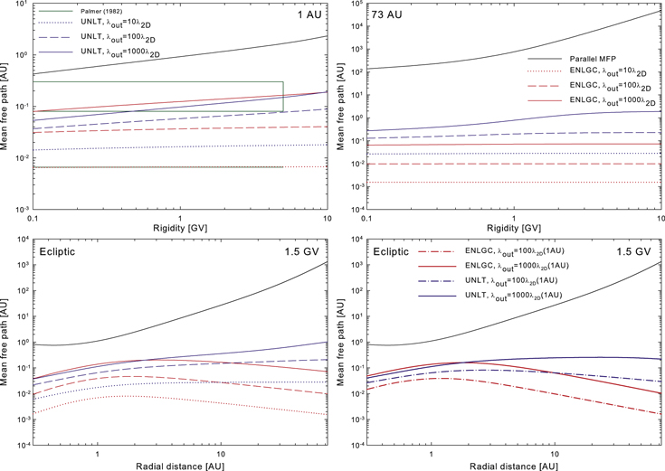
Figure 6. Proton parallel and perpendicular mean free paths employed in this study, shown as a function of rigidity at 1 and 73 AU (top left and right panels) and as a function of heliocentric radial distance in the solar ecliptic plane at a rigidity of 1.5 GV (bottom panels), for the various forms assumed in this study for the 2D outerscale λout. Palmer (1982) consensus values for the parallel and perpendicular MFPs are shown in the top left panel for 1 AU. Note that the legend for the bottom right panel differs from those of the other three panels.
Download figure:
Standard image High-resolution image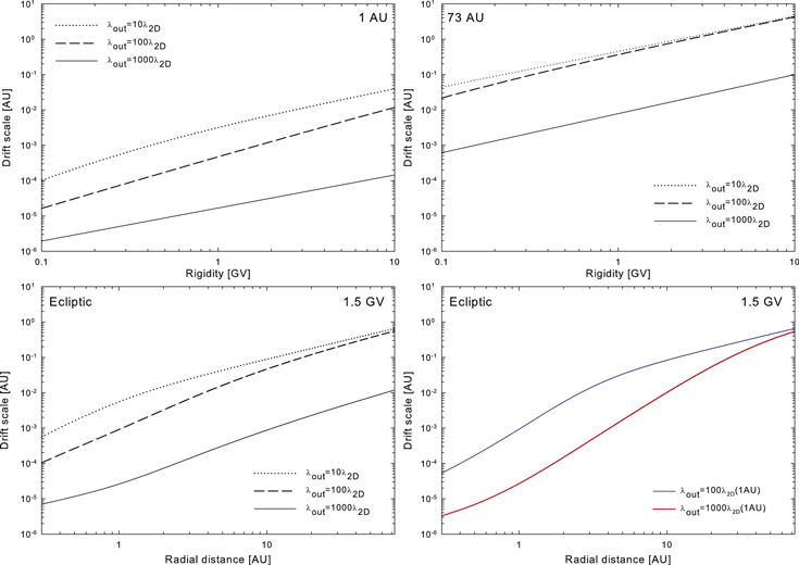
Figure 7. Proton drift scales employed in this study, shown as a function of rigidity at 1 and 73 AU (top left and right panels) and as a function of heliocentric radial distance in the solar ecliptic plane at a rigidity of 1.5 GV (bottom panels), for the various forms assumed in this study for the 2D outerscale λout.
Download figure:
Standard image High-resolution imageTurning now specifically to the results presented here regarding the perpendicular mean free paths in Figure 6, it is clear that the choice of λout has a significant effect on λ⊥ for both scattering theories at all rigidities shown and at both radial distances considered, with values for λ⊥ ranging, at Earth, from values in excellent agreement with Palmer consensus values for the perpendicular mean free path (ENLGC case with λout = 10λ2D) to well within the Palmer consensus range for the parallel mean free path (both theories, for λout = 1000λ2D). At 73 AU, the range of perpendicular mean free path values spanning from the largest (UNLT case with λout = 1000λ2D) to the smallest (again the ENLGC case with λout = 10λ2D) covers almost three orders of magnitude. Results derived from the UNLT for a particular value of λout tend to be larger than those derived using the ENLGC theory for a given value of the 2D outerscale. One exception to this behavior is the case where λout = 10λ2D, at least until ∼2 AU, as can be seen from the bottom panels of Figure 6. Beyond this distance, the UNLT λ⊥ are consistently larger than the ENLGC λ⊥.
Comparison of the drift scales as a function of rigidity at Earth and 73 AU in the top panels of Figure 7 show that larger outerscales lead to smaller λA. This quantity is also very sensitive to the value used for λout, varying by almost two orders of magnitude as a function of rigidity across the range of values for λout considered in the top two panels of Figure 7. Note, however, that at the highest rigidities shown (above ∼2 GV at 1 AU), and at all rigidities at 73 AU, the drift scales for the cases where λout = 10λ2D and λout = 100λ2D reach very similar values, with those for the former close displaying a ∼P rigidity dependence like that expected of the weak scattering result, where λA = RL. The bottom panels of Figure 7 show the radial dependences of the 1.5 GV drift scales calculated using the forms for λout given in Equations (29) and (30). For the case where the outerscale is always 1000 times larger than λ2D, the drift scale at ∼70 AU is ∼100 times larger than for the case where the outerscale is constant at 100 times the value of λ2D at Earth. The difference between the two cases decreases significantly when the outerscale is decreased by a factor of 10.
5. COMPUTED INTENSITIES
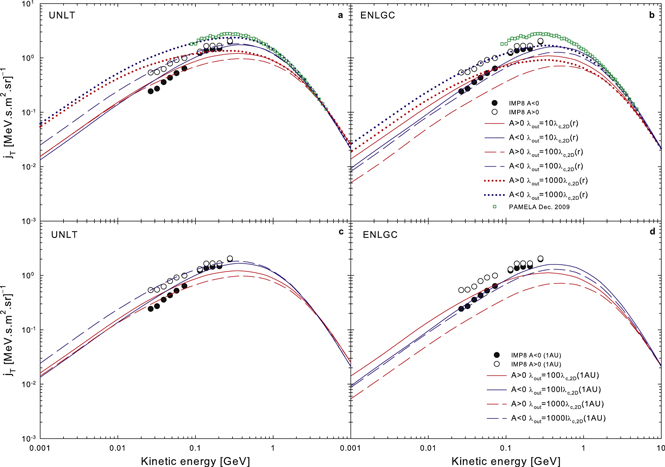
Using the above diffusion and drift coefficients, with results from the Oughton et al. (2011) TTM as inputs for basic turbulence quantities, the SDE code presented here is used to compute galactic CR proton intensities at Earth for the various forms of 2D outerscale described by Equations (29) and (30). This modulation code is run for generic solar minimum values for both large-scale heliospheric quantities such as the solar wind speed profile and HMF magnitude, as well as for generic solar minimum values for small-scale quantities pertaining to turbulence, as described in Section 2, using the observationally motivated spectra discussed in the same section as input at 73 AU (Equations (10) and (11)). Note that the number of pseudo-particles in the SDE code is set at N = 5000 in the following. Figure 8 shows these intensities, computed for both positive (red lines, A > 0) and negative (blue lines, A < 0) magnetic polarity cycles, as a function of kinetic energy using perpendicular mean free path expressions derived from the UNLT (left panels) and ENLGC theories (right panels). Observed galactic proton spectra reported by McDonald et al. (1992) and Potgieter et al. (2013) are also shown. The legend in the top right panel applies to all the panels except the bottom right one, which is provided with its own legend.
Figure 8. Galactic cosmic ray proton differential intensities at 1 AU computed using the SDE ab initio modulation code for different assumed 2D outerscales during positive (red lines) and negative (blue lines) magnetic polarity cycles. The left panels show results calculated using a perpendicular mean free path expression derived from the UNLT, while the right panels show results computed using an ENLGC perpendicular mean free path expression. Data shown are taken from McDonald et al. (1992) and Potgieter et al. (2013).
Download figure:
Standard image High-resolution image
In general, intensities computed using UNLT perpendicular mean free paths are larger than their ENLGC counterparts. This reflects the general trend seen in Figure 6, where UNLT perpendicular mean free paths tend to be larger than ENLGC mean free paths for a given λout. The large effect of changes in λout on the perpendicular mean free paths and drift scales translates to large differences in the corresponding computed CR intensity spectra, but it is interesting to note that all the computed spectra remain quite close to the observations shown in Figure 8. Note that solutions for A > 0 are larger than those for A < 0, as shown by observations, only for the smallest value of the outerscale considered in each panel. However, the crossover in intensities, for both the UNLT and ENLGC results, occurs at energies below those at which this phenomenon is observed to occur. For the cases where λout is assumed to be a constant multiple of the 2D correlation scale yielded by the Oughton et al. (2011) TTM as this quantity varies with radial distance, use of the smallest outerscales (with λout = 10λ2D(r)) yields results quite close to the IMP8 observations for both A > 0 and A < 0, with particularly good agreement for the ENLGC intensities during A < 0. For this choice of λout, the A > 0 and A < 0 intensity spectra cross over at an energy slightly below ∼0.2 GeV, with A < 0 intensities then being larger at higher energies, in qualitative agreement with neutron monitor observations (see, e.g., Reinecke & Potgieter 1994 and Potgieter et al. 2001). Similar behavior occurs for the case where λout = 10λ2D(1 AU), for both scattering theories (panels (c) and (d) of Figure 8). Interestingly, spectra computed using ENLGC perpendicular mean free paths with λout = 100λ2D(r) (panel (b) of Figure 8) are lower than those computed using λout = 10λ2D(r), a situation not seen for the UNLT results in panel (a) of the same figure. This is probably due to the fact that at greater radial distances, the drift scale is larger relative to the ENLGC perpendicular mean free path than to the UNLT perpendicular mean free path for this particular choice of outerscale. For the case where λout = 100λ2D(1 AU), the intensities computed using both UNLT and ENLGC mean free paths appear very nearly the same as those computed assuming that λout = 10λ2D(r): as shown in Figure 5, both these choices for λout lead to similar values for this quantity, and hence to similar values for the transport parameters it influences, at large radial distances. Lastly, intensities computed using both scattering theories while assuming that λout = 1000λ2D(r) are considerably higher than those computed for smaller λout, with A > 0 intensities again falling below A < 0 intensities. Intriguingly, the A < 0 intensities computed using UNLT perpendicular mean free paths agree rather well with the unusually high A < 0 proton intensities observed by PAMELA in 2009 December. This agreement extends to the lower energy PAMELA observations, which display an energy dependence somewhat different to that shown by the IMP8 observations. This may be due to the slightly steeper rigidity dependence of the perpendicular mean free paths calculated using λout = 1000λ2D(r), as shown in Figure 6.
6. DISCUSSION AND CONCLUSIONS
The ab initio SDE CR modulation code presented here combines such an approach for the first time with a TTM, and was benchmarked against a modulation code that utilizes an ADI numerical solver with identical transport parameters for the Parker transport equation. From Section 5, it is clear that computed galactic CR proton intensities are extremely sensitive to the low-wavenumber behavior of the 2D turbulence power spectrum, as well as to the choice of scattering theory employed in the derivation of the perpendicular diffusion coefficient. This is, of course, due to the sensitivity of this diffusion coefficient, as well as that of the turbulence-reduced drift coefficient considered here to assumptions made as to the energy-containing range on the 2D power spectrum.
From Figure 8, it can be seen that only results calculated assuming a 2D outerscale that is only moderately larger than the 2D turnover scale agree qualitatively with what is expected of spacecraft observations at Earth during periods of "usual" solar activity, as represented by the IMP8 observations shown in the same figure. Also, the computed intensities appear to be most sensitive to the values of λout at larger radial distances. This would imply that, given solar minimum conditions such as those observed before the unusual solar minimum in 2009, the extent of the energy-containing range on the 2D spectrum at large radial distances would be less than an order of magnitude in wavenumber. This could possibly be tested by an analysis of Voyager observations such as that presented by Fraternale et al. (2015). These authors, however, note that the Voyager 2 data displays many gaps, which could complicate such an analysis. An investigation of second-order structure functions (see, e.g., Miranda et al. 2012; Ni & Xia 2013 and Wicks et al. 2013) calculated using these observations may, however, prove to be useful in this regard. Galactic CR proton intensities calculated with larger values for λout appear to not qualitatively agree with the IMP8 observations at all, especially with regards to the fact that intensities computed for A < 0 magnetic polarity cycles are larger than those computed for A > 0 conditions. However, the A < 0 solution calculated using UNLT perpendicular mean free paths for the case where λout = 1000λ2D(r) agree very well with the unusually high intensities detected by PAMELA during the (A < 0) solar minimum of 2009. Perpendicular mean free paths calculated under the assumption that λout = 1000λ2D(r) also display a rigidity dependence (see Figure 6) quite different to those shown by perpendicular mean free paths calculated assuming smaller 2D outerscales. This is reminiscent of the findings of Potgieter et al. (2013), who fit various CR proton intensity spectra observed by PAMELA by changing the rigidity dependence of the parametric parallel mean free path expression they employ, although these authors find that a flatter rigidity dependence is needed to fit the 2009 intensity spectra. Given that the values for λout yielded by this choice at large radial distances are probably unrealistic, this could be seen to be problematic. However, spacecraft observations of turbulence quantities such as the magnetic variance have been reported to display a solar cycle dependence (see, e.g., Bieber et al. 1993; Smith et al. 2006a; Burger et al. 2014). The TTM used in this study is set up to yield turbulence quantities in agreement with observations taken during generic solar minimum conditions. Burger et al. (2014) report that during the unusual 2009 solar minimum, turbulence quantities behaved differently than during other solar minima, echoing the unusual behavior of the HMF during this period. From the bottom panel of Figure 5, it is clear that, holding all other turbulence quantities constant, increasing the value of the outerscale acts to lower the levels of the resulting 2D spectra relative to each other for wavenumbers above ∼1.4 AU−1. Note that these wavenumbers correspond roughly to the Larmor radii of galactic CR protons with rigidities in the range of interest to this study. From Equation (15) this effect could, however, be reproduced by holding λout at some constant value, and varying the value of  The implication then is that it is the level of the 2D turbulence power spectrum at large radial distances that is having such a marked effect on computed CR intensities. As Burger et al. (2014) report an unusually low value for the variance during 2009, it is then plausable that the lower spectral level during this period may be the cause of the unusually high observed CR intensities. Finally, as discussed in the previous section, the smallest values of the outerscale used here lead to results at least in qualitative agreement with spacecraft observations, although the crossover between intensities computed for A > 0 and A < 0 conditions occurs at too low energies for both scattering theories considered. Runs for even smaller values of the outerscale considered here do not lead to better agreement with observations. This may be due to at least two reasons. First, a more thorough understanding of the effects of turbulence on the drift coefficient may resolve this issue, in that the turbulence-reduced drift coefficient employed here may not be realistic for turbulence conditions prevalent in the fast solar wind (see Engelbrecht & Burger 2013b for more detail). Second, this study does not take into account any polarity cycle dependence in the diffusion coefficients. Separate studies of neutron monitor data by Chen & Bieber (1993) and Munakata et al. (2014) both find that the solar minimum parallel mean free path during A < 0 is larger than during A > 0. As the perpendicular mean free paths presented here are functions of λ∥, taking this into account would affect the computed proton intensities presented here. Third, whereas a steady state is assumed in the present study, a fully time-dependent approach is likely to change the results as well. In this case, intensities during solar minimum are actually determined by conditions in the period preceding solar minimum. This would require knowledge of the solar cycle dependence of all of the turbulence quantities required for modulation models, not all of which have been studied in sufficient detail (Burger et al. 2014).
N.E.E. thanks R. D. Strauss for many valuable discussions. This work is based on research supported in part by the National Research Foundation of South Africa (Grant Numbers 81834, 93592, and 96478). N.E.E. acknowledges support by the South African National Space Agency.