


ABSTRACT
Studies of planets in binary star systems are especially important because it was estimated that about half of binary stars are capable of supporting habitable terrestrial planets within stable orbital ranges. One-planet binary star systems (OBSS) have a limited analogy to objects studied in atomic/molecular physics: one-electron Rydberg quasimolecules (ORQ). Specifically, ORQ, consisting of two fully stripped ions of the nuclear charges Z and Z' plus one highly excited electron, are encountered in various plasmas containing more than one kind of ion. Classical analytical studies of ORQ resulted in the discovery of classical stable electronic orbits with the shape of a helix on the surface of a cone. In the present paper we show that despite several important distinctions between OBSS and ORQ, it is possible for OBSS to have stable planetary orbits in the shape of a helix on a conical surface, whose axis of symmetry coincides with the interstellar axis; the stability is not affected by the rotation of the stars. Further, we demonstrate that the eccentricity of the stars' orbits does not affect the stability of the helical planetary motion if the center of symmetry of the helix is relatively close to the star of the larger mass. We also show that if the center of symmetry of the conic-helical planetary orbit is relatively close to the star of the smaller mass, a sufficiently large eccentricity of stars' orbits can switch the planetary motion to the unstable mode and the planet would escape the system. We demonstrate that such planets are transitable for the overwhelming majority of inclinations of plane of the stars' orbits (i.e., the projections of the planet and the adjacent start on the plane of the sky coincide once in a while). This means that conic-helical planetary orbits at binary stars can be detected photometrically. We consider, as an example, Kepler-16 binary stars to provide illustrative numerical data on the possible parameters and the stability of the conic-helical planetary orbits, as well as on the transitability. Then for the general case, we also show that the power of the gravitational radiation due to this planet can be comparable or even exceed the power of the gravitational radiation due to the stars in the binary. This means that in the future, with a progress of gravitational wave detectors, the presence of a planet in a conic-helical orbit could be revealed by the noticeably enhanced gravitational radiation from the binary star system.
Export citation and abstract BibTeX RIS
1. INTRODUCTION
Stability of planetary systems is the subject of a continuing interest. One reason is that it is related to the search for habitable planets. Studies of planets in binary star systems are especially important because it was estimated that about half of binary stars are capable of supporting habitable terrestrial planets within stable orbital ranges (see, e.g., David et al. 2003; Fatuzzo et al. 2006; Quintana & Lissauer 2010, pp. 265–283).
One-planet binary star systems (hereafter, OBSS) have a limited analogy to objects studied in atomic/molecular physics: one-electron Rydberg quasimolecules (hereafter, ORQ). Specifically, ORQ, consisting of two fully stripped ions of the nuclear charges Z and Z' plus one highly excited electron, are encountered in various plasmas containing more than one kind of ion. Examples are (but not limited to) magnetic fusion plasmas, laser-produced plasmas, plasmas used for X-ray and VUV lasers, and solar plasmas. In these plasmas, a fully stripped ion of the nuclear charge Z' can come close to a hydrogen-like ion of the nuclear charge Z and form a short-lived molecule (i.e., a quasimolecule). Conversely, a fully stripped ion of the nuclear charge Z can come close to a hydrogen-like ion of the nuclear charge Z' and form a quasimolecule. Such quasimolecules are a very useful playground for theoretical and experimental studies of charge exchange, which is a physical process of primary importance for many areas of physics (e.g., for the areas listed above).
Classical analytical studies of ORQ were presented in two papers (Oks 2000a, 2000b) and later also in the book (Oks 2006, Appendix A). The primary result was the discovery of classical stable electronic orbits of the shape of a helix on the surface of a cone.
In the present paper we show that stable helical orbits are possible for OBSS. The overwhelming majority of papers on planetary orbits around binary stars considered only various types of planetary motion in the orbital plane of the two stars (see, e.g., Innanen et al. 1997; Holman & Wiegert 1999; David et al. 2003; Turrini et al. 2005; Fatuzzo et al. 2006; Desidera & Barbieri 2007; Quintana et al. 2007; Quintana & Lissauer 2010, pp. 265–283; Kaib et al. 2013, and references in those publications)—to the best of our knowledge. In this paper we present the motion of a planet, roughly speaking, in the plane perpendicular to the interstellar axis—more rigorously, the planet orbit is a helix on a conical surface, whose axis of symmetry coincides with the interstellar axis.
There is only a limited similarity between ORQ and OBSS because of the following distinctions between these two physical systems. First, in ORQ the attractive centers (nuclei Z1 and Z2 can be stationary and still be stable, while in binary star systems the rotation of the stars is necessary for the stability.
Second, in ORQ the attractive centers can engage in oscillations (called vibrations) and be stable without any rotation. This is not the case for OBSS.
Third, in ORQ the electronic degrees of freedom have a much larger characteristic frequency and energy than the nuclear degrees of freedom. This is the basis for the standard Born–Oppenheimer approximation, where the primary contribution to the energy of the system can be obtained by freezing the nuclear motion. If necessary, the nuclear motion can then be taken into account by perturbation theory.
The Born–Oppenheimer approximation is a particular case of the general analytical method for a system that can be separated into rapid and slow subsystems. For ORQ, this method is applicable because the ratio of frequencies (and energies) of the electronic motion, the vibrational nuclear motion, and the rotational nuclear motion is 1:  :(me/
:(me/ . Here me is the electron mass and Mn is the total mass of the two nuclei, so that me/Mn < 1/3600 and the separation of the slow and rapid subsystems is justified automatically. This is, generally speaking, not the case for OBSS.
Indeed, for OBSS the analogue of molecular oscillations (vibrations) is a periodic change of the separation between the two stars, which occurs for eccentric stellar orbits. One distinction from ORQ is that both oscillations and rotations have the same frequency: the Kepler frequency ω of the two stars orbiting their barycenter. Another distinction from ORQ is that the primary frequency Ω of the helical motion of the planet is not automatically much greater than the stars' Kepler frequency ω.
In the present paper we demonstrate that there are ranges of parameters where  Further, we show that in these ranges, the planetary motion is stable—both for a model case of stationary stars and for the real case of stars rotating in circular orbits. We demonstrate that the allowance for the eccentricity of stars' orbits does not affect the stability of the conic-helical planetary motion if the center of symmetry of the helix is relatively close to the star of the larger mass. We also show that if the center of symmetry of the conic-helical planetary orbit is relatively close to the star of the smaller mass, a sufficiently large eccentricity of stars' orbits can switch the planetary motion to the unstable mode and the planet would escape the system. Finally, we demonstrate that such planets are transitable for the overwhelming majority of inclinations of the plane of the stars' orbits (i.e., the projections of the planet and the adjacent start on the plane of the sky coincide once in a while). This means that conic-helical planetary orbits at binary stars can be detected photometrically.
We consider, as an example, Kepler-16 binary stars to provide illustrative numerical data on the possible parameters and the stability of the conic-helical planetary orbits. We also show that such planetary orbits at Kepler-16 would be transitable.
Then for the general case we also demonstrate that the power of the gravitational radiation due to this planet can be comparable or even exceed the power of the gravitational radiation due to the stars in the binary. This means that in the future, with a progress of gravitational wave detectors, the presence of a planet in a conic-helical orbit could be revealed by the noticeably enhanced gravitational radiation from the binary star system.
The paper is organized as follows. In Section 2 we consider a model case where two stars are stationary and study the stability of the nearly circular orbit of a planet, where the axis of symmetry of the planetary orbit coincides with the interstellar axis. We find ranges of parameters where the orbit is stable and has the conic-helical shape. This model case is analogous to the analytical results concerning ORQ from Oks (2000a, 2000b). In Section 3 we analyze a real situation. Namely, we take into account the rotation of the two stars, as well as the eccentricity of their orbits, and study the effects of the rotation and the eccentricity on the stability of the conic-helical orbit of the planet. The results of Section 4 have no analogues in studies of ORQ. In Section 5 we discuss the detection of planets in conic-helical orbits at binary stars. In Section 5 we present conclusions.
2. MODEL CASE: A CONIC-HELICAL ORBIT OF A PLANET AT TWO STATIONARY STARS
2.1. Points of a Dynamical Equilibrium
In this section we start by considering a model system consisting of two immobile stars of masses μ and μ', and a planet of a unit mass moving around a circle in the plane perpendicular to the interstellar axis on which the circle is centered. The mass μ is at the origin and the Oz axis is directed to the mass μ' located at z = R. We introduce notations

where G is the gravitational constant. The Hamilton function can be written in the cylindrical coordinates  as follows.

The last term in Equation (2) is the potential energy:

The Hamiltonian equations of the motion relate the momenta and the velocities:
Since  is the cyclic coordinate, the corresponding momentum is conserved:

Physically, the quantity M is a projection of the planet angular momentum on the interstellar axis. Thus, we can separate the z- and ρ-motions from the  -motion. So after solving the z- and ρ-motions, we can find the
  -motion using Equation (5) where M is the separation constant.
The separated z- and ρ-motions can be described by the following Hamilton function.

The last term in Equation (6) is an effective potential energy:

Now we define scaled (dimensionless) variables w and v, a scaled projection of the angular momentum m, as well as a ratio of the star masses b:

In the scaled notations, the effective potential energy can be represented in the form
In equilibrium, the derivatives of Ueff by both scaled coordinates  must vanish. By setting to zero the partial derivative of Ueff by w:

we obtain the relation:

This relation determines a line v0(w) in the plane (w, v), which is the locus of the equilibrium points:
The equilibrium points exist in the following regions of w:
- A.for
 , the regions are 0 w 1/ and b/(1+b) < w 1;
 - B.for, the regions are and 1/ w 1;
- C.for b = 1, the region is the entire range of 0 w 1.


In the rest of the paper we call these intervals the "allowed ranges" of w. As an example, Figure 1 shows the dependence v0(w) for b = 3.
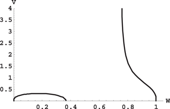
Figure 1. Dependence of the equilibrium value of the scaled radius  of the planetary orbit on the scaled axial coordinate
  of the planet for the ratio of the stellar masses μ'/μ = 3.
Download figure:
Standard image High-resolution imageNow we set to zero the partial derivative of Ueff by v:

On substituting v0(w,b) from Equation (12) instead of v, we obtain
In the course of the derivation of Equation (14), we employed Equation (11) for removing the explicit dependence on b. As a result, the stellar mass ratio b shows up in Equation (14) only as the argument of the function v0(w, b). In the following we will also use Equation (11) for this purpose in similar derivations without further notice.
For each pair (w, b), where w belongs to the allowed ranges, Equation (12) specifies the equilibrium value v0(w, b), while Equation (14) specifies the equilibrium value m0(w, b). As an example, Figure 2 shows the dependence m0(w) for b = 3.
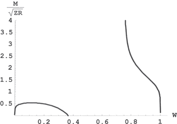
Figure 2. Dependence of the equilibrium value of the scaled projection of the planet angular momentum 
 on the interstellar axis versus the scaled coordinate
  of the planet along the interstellar axis for the ratio of the stellar masses μ'/μ = 3.
Download figure:
Standard image High-resolution imageEquivalently, for a pair (b, m), solving Equation (14) produced one or more values of wi(b, m). Subsequently, Equation (12) specifies the values vi = v0(wi(b, m), b). The result is pairs (wi, v corresponding to equilibria. So, for each ratio of the stellar masses b, there are pairs of equilibrium values (wi, v
 , m
, m . Here v
 v0(w
v0(w , m
, m m0(w
m0(w , where wi is taken from the allowed ranges.
2.2. Analytical Solution for the Three-dimensional Motion
Now for some value of b, we consider small deviations from equilibrium values (wi, v , m
, m :
:

By expanding the scaled effective potential energy ueff in terms of δw and δv, we get
where
Here the suffix 0 at the derivatives means that after the differentiation one should set v = v0(w) and m = m0(w). (For brevity we dropped the suffix i.) The following notations are used in Equation (17).
For transforming the effective potential energy ueff to so-called normal coordinates, which would diagonalize the matrix composed of the second derivatives of ueff in the general case where u 0, we rotate the reference frame:

The angle of the rotation, achieving the diagonalization, satisfies the condition

so that
The effective potential energy can be written in the normal coordinates as follows.

where

It should be emphasized that  , which is the scaled frequency of small oscillations in the direction of the normal coordinate δv', is always real. Hereafter, any frequency F and its scaled counterpart f are interconnected by the following relation.

Concerning the other eigenfrequency  , it is real under the condition

On substituting Q from Equation (18), the inequality (25) can be reformulated as follows.
When the inequality (26) is met, the quantity  is the frequency of small oscillations in the direction of the normal coordinate δw'.
We arrive to the conclusion that, if v0(w, b) > vcrit(w), the effective potential energy has a two-dimensional minimum at the equilibrium values of w and v = v0(w, b). In other words, if v0(w, b) > vcrit(w), the equilibrium is stable. After defining a scaled (dimensionless) time of

the resulting expression for the small oscillations around the stable equilibrium can be represented by the following formulas.
Here sin α and cos α are determined by Equation (21), while amplitudes aw, av and phases  ,
,  —by initial conditions.
Now we rewrite Equation (5) in the scaled notations as

and substitute in  v
v , where the quantity
  is defined by Equation (29). Then we integrate it over τ and find the following solution for the
  -motion
Here the quantity

is a scaled primary frequency of the  -motion (the primary frequency of the
  -motion in the usual units of 1 s−1 is denoted as
  ).
).
Equations (30) and (31) demonstrate that the  -motion is a rotation about the interstellar axis with the frequency f, slightly modulated by oscillations of the scaled radius of the orbit v at the frequencies
  and ω. Thus, for the stable motion, the planetary trajectory is a helix on the surface of a cone, with the axis coinciding with the interstellar axis. In this conic-helical state, the planet, while spiraling on the surface of the cone, oscillates between two end-circles that result from cutting the cone by two parallel planes perpendicular to its axis (Figure 3).
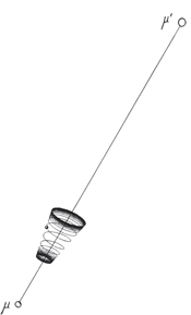
Figure 3. Sketch of the conic-helical motion of the planet in the model binary star system. We stretched the trajectory along the interstellar axis to make its details better visible.
Download figure:
Standard image High-resolution imageThe scaled eigenfrequencies  and
and  of the zρ-motion and the scaled frequency fp of the
  -motion are related as follows.

Thus, the eigenfrequencies of the zρ-motion are generally of the same order of magnitude as the frequency of the  -motion.
2.3. Classical Energy Terms
From this point on, the projection M of the planet orbital momentum on the interstellar axis will be fixed. We analyze the behavior of the energy at M = const > 0 (it is sufficient to consider only M > 0 because the results for M and -M are physically the same). In the analogous quantal problem of ORQ, this means studying "terms of the same symmetry."
Combining the definition of  from Equation (8) with (14), we get

Now the coordinates z and  can be represented as z(w, b, M) = wR(w, b, M) and
  (w, b, M) = v
 (w, b)R(w, b, M). For any b > 0, for any w from the allowed ranges (controlled by the value of b), and for any M > 0, the functions R(w, b, M), z(w, b, M), and
  (w, b, M) determine the equilibrium values of the interstellar distance R, the location of the orbital plane z, and the radius of the orbit
  , respectively.
For simplicity, we neglect the small oscillations of the z- and  -coordinates and concentrate on the primary
  -motion, where the planet moves around the circle of the radius
  (w, b, M) = v
 (w, b)R(w, b, M). Then the total energy E of the planet is the same as the effective potential energy presented by Equation (7):

In the spirit of notations in Equation (9), we define a scaled total energy e in the following way:
By employing Equations (11) and (14), the scaled total energy can be represented as
By substituting R(w, b, M) from Equation (33) in (35), we obtain:

Here we take a fresh look at the combination of Equations (33) and (37). For any b > 0 and M  0, they determine in a parametric form (w being the parameter) the dependence of the energy E on the interstellar distance R. Borrowing the terminology from the analogous quantal problem, this dependence is called classical energy terms.
The plot of the scaled energy (M/Z)2E versus the scaled interstellar distance (Z/M2)R is presented in Figure 4 for the ratio of the stellar masses b = 3. There are three classical energy terms corresponding to the same value of M and two of them cross.
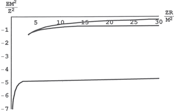
Figure 4. Classical energy terms: the dependence of the scaled energy  of the planet on the scaled interstellar distance
  R for the ratio of the stellar masses μ'/μ = 3.
Download figure:
Standard image High-resolution imageThis example, given for the ratio of the stellar masses μ'/μ = 3, actually represents a typical situation. We found that for any pair of μ and  there are three classical energy terms of the same symmetry and the upper term always crosses the middle term. (For μ' = μ there is only one term in the corresponding plot and no crossing—as should be expected.)
The origin of these three classical energy terms can be determined for any ratio of the stellar masses  . At R
  , the lower term corresponds to the energy of the planet around a single star of the mass
  , (E
, (E  /2), slightly perturbed by the star of the mass
  min
min  . The planet is in the state corresponding to the zero projection A
 of the Runge–Lenz vector [13] on the interstellar axis. At R
  0, the lower term corresponds to the energy of the planet around an effective single star of the mass
  , (E
, (E ![$\to -{{[G(\mu +\mu ^{\prime} )/M]}^{2}}$](https://content.cld.iop.org/journals/0004-637X/804/2/106/revision1/apj511242ieqn67.gif) /2).
/2).
At R  , the middle term corresponds to the energy of the planet around a single star of the mass
  , (E
, (E  −
− /2), slightly perturbed by the star of the mass
  max
max  . The planet is in the state corresponding to A
 = 0.
= 0.
At R  , the upper term corresponds to a near-zero-energy state where the planet is almost free. In terms of the parameter w, this term at
  corresponds to
  .
.
At the crossing of the middle and upper energy terms, the eigenfrequency  , defined by Equation (23), vanishes. The middle term corresponds to stable equilibria of the three-dimensional planetary motion, while the upper term corresponds to unstable equilibria of the three-dimensional planetary motion. The value of wc corresponding to the crossing can be found in any of the following three: E'
 = 0, M'
 = 0 (where the symbol ' stands for the derivative), or

where the critical value of the scaled radius of the planetary orbit vcrit(w) was defined by Equation (26). While solving any of those three equations, only the root wc within the interval (0, 1) should be accepted; in other words, the values 0 and 1 (the endpoints) should be excluded.
3. REAL SYSTEM: EFFECTS OF THE STARS ROTATION AND THE ECCENTRICITY OF THEIR ORBITS ON THE CONIC-HELICAL ORBIT OF THE PLANET
3.1. Validity of the Separation in Rapid and Slow Subsystems
The Kepler frequency ω of the two stars orbiting their barycenter is

This is also the frequency of oscillations of the interstellar distance in the case of eccentric stellar orbits. According to Equation (24), the scaled, dimensionless counterpart of the Kepler frequency is

where we used the previously introduced notations Z = G and b =
  '/
'/ . The ratio of the scaled primary frequency f
 of the planetary motion (given by Equation (31)) to the scaled Kepler frequency f
 of the stars is
As an example, Figure 5 shows the dependence r(w) for the ratio of the stellar masses b = 3. It is seen that this ratio becomes sufficiently large if the projection of the planetary orbit on the interstellar axis is either close to the star of smaller mass ( ) or close to the star of larger mass ((1 − w)
  ).
).
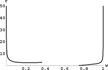
Figure 5. Ratio r of the frequencies of the rapid and slow subsystems versus the scaled projection w of the planetary orbit on the interstellar axis for the ratio of the stellar masses b = 3.
Download figure:
Standard image High-resolution imageWe denote by  the scaled critical distance between the projection of the planetary orbit on the interstellar axis and the star of the smaller mass, such that at
  we have the ratio of the two frequencies r > 10. Similarly we denote by
  the scaled critical distance between the projection of the planetary orbit on the interstellar axis and the star of the larger mass, such that at (1 − w)
  we have the ratio of the two frequencies r > 10. Figures 6 and 7 show the dependence of
  and
and  , respectively, on the ratio of the stellar masses b.
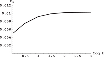
Figure 6. Scaled critical distance D1 between the projection of the planetary orbit on the interstellar axis and the star of the smaller mass (such that at w < D1 the ratio of the frequencies of the rapid and slow subsystems is r > 10) versus the decimal logarithm of the ratio b of the stellar masses.
Download figure:
Standard image High-resolution image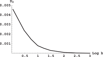
Figure 7. Scaled critical distance D2 between the projection of the planetary orbit on the interstellar axis and the star of the larger mass (such that at (1 − w) < D2 the ratio of the frequencies of the rapid and slow subsystems is r > 10) versus the decimal logarithm of the ratio b of the stellar masses.
Download figure:
Standard image High-resolution imageIt is seen that as the ratio b of the stellar masses increases, the scaled critical distance  also increases, whereas the scaled critical distance
  decreases. The most important thing to note here is that there are ranges of parameters where the separation into the rapid and slow subsystems is justified, and those ranges are clearly shown in Figures 6 and 7 for any ratio of the stellar masses.
3.2. The Effect of the Stars Rotation
In the reference frame rotating together with the stars with the Kepler frequency  , the Hamilton function of the planet acquires an additional term –
![${\boldsymbol{r}} \;\cdot \;[{\boldsymbol{p}} \;\times \;{\boldsymbol{ \omega }} ]$](https://content.cld.iop.org/journals/0004-637X/804/2/106/revision1/apj511242ieqn97.gif) and becomes (see, e.g., Landau & Lifshitz 1960)
and becomes (see, e.g., Landau & Lifshitz 1960)

where

This leads to an additional (Coriolis) force

Because v  —where
  is the primary frequency of the planetary motion and
  is the average radius of the planetary orbit—and
  , then the additional force is approximately

Expression (45) has a clear physical meaning for the quantal counterpart-problem of ORQ. Namely, it is a Lorentz electric field  /c in the effective magnetic field
  in atomic units (or
  in the CGS units, m
 being the electron mass).
We choose the Ox axis along vector  , which is obviously perpendicular to the interstellar axis chosen as the Oz axis. Because the planetary velocity
  is primarily in the xy-plane perpendicular to the interstellar axis, then the additional force
  is primarily along the interstellar axis.
A more accurate calculation is as follows. Representing  , we get
  +
+  . Because
  , we obtain from Equation (44):

In the ranges of parameters where  , Equation (46) becomes

Thus, for the z -motion (which in the scaled coordinates is wv-motion), the situation represents a two-dimensional oscillator, having the scaled eigenfrequencies
  and
and  defined by Equation (23), which is driven by the force
  oscillating at the frequency
  . Using the well-known formulas for driven oscillators (see, e.g., Jose & Saletan 1998), the solution in the coordinates w', v' rotated by the angle
  (defined by Equation (20)) compared to the coordinates w, v (i.e., in the coordinates, where the two oscillators are decoupled), can be written as follows.
Here f is the scaled primary frequency of the planetary motion defined by Equation (31),
  is the scaled time defined by Equation (27), and
  is the scaled Kepler frequency of the stars' rotation:

In the original scaled coordinates w, v, the forced oscillations are
Using the relation (32), the latter formulas can be rewritten as follows.
In the ranges of parameters where  , and consequently f
 , and given that
  and f
and f are generally of the same order of magnitude (according to Equation (32)), it is seen from Equation (50) that the forced oscillation of the planetary orbit occurs with a relatively small amplitude. Thus, the rotation of the stars does not affect the stability of the planetary orbit.
3.3. The Effect of the Eccentric Orbits of the Stars
In the reference frame rotating together with the stars with the Kepler frequency  , a non-zero eccentricity
  of the stars' orbits results in the oscillation of the interstellar distance R with the frequency
  . In the ranges of parameters where
  , the oscillation of the interstellar distance is an adiabatic perturbation of the planetary motion. According to the principle of adiabatic invariance, the planetary motion will adjust to the slowly varying R while keeping as the constant the projection of the planetary angular momentum M on the interstellar axis (M is the adiabatic invariant).
The classical energy terms, such as those presented in Figure 4, correspond to the situation where M is a constant. Consequently, as a result of the eccentricity of the stars' orbits, the state of the planetary motion will adiabatically oscillate along a particular energy term E(R).
The entire lower energy term, which relates to the situation where the center of symmetry of the conic-helical planetary orbit is relatively close to the star of the larger mass, corresponds to a stable planetary motion. So, the eccentricity of the stars' orbits cannot affect the stability of the planetary motion in this case.
The middle energy term, which relates to the situation where the center of symmetry of the conic-helical planetary orbit is relatively close to the star of the smaller mass, is also the zone of stability as long as R > Rc, where Rc is the interstellar distance where the middle energy term crosses the upper energy term. For the state of the planetary motion corresponding to the middle energy term, the planetary motion would remain stable if, in the course of the oscillation along the middle energy term, the system could not reach R = Rc. However, if in the course of the oscillation along the middle energy term the system did reach R = Rc, the planetary motion would switch to the upper energy term corresponding to the unstable mode and the planet would be able to escape the system.
The stability of the conic-helical planetary orbit close to the star of the smaller mass can be also understood and analyzed quantitatively using Figure 2. This Figure depicts the dependence of the scaled projection of the planet angular momentum m ≡ M/(ZR) on the interstellar axis versus the scaled averaged coordinate w ≡ z/R of the planet orbital plane along the interstellar axis. The left branch of this dependence reaches its maximum value m
 at w = wc, corresponding to the crossing of the middle and upper energy terms in Figure 4. Values of m at w < wc correspond to the stable motion. Under the condition that the orbital frequency of the planet is much greater than the Kepler frequency of the stars, at the average interstellar distance
  , the values of w and m are such that w <
  and m <
  (
( was defined before Figure 6 and in the caption to Figure 6). The point with coordinates w =
  and m = m(
 in Figure 2 is very close to the origin. As R decreases to its minimum value R
 , while M and Z remain constant, the value of m increases
 ![${{[\langle R\rangle /{{R}_{{\rm min} }}]}^{1/2}}$](https://content.cld.iop.org/journals/0004-637X/804/2/106/revision1/apj511242ieqn140.gif) times: the corresponding point in Figure 2 moves up along the ascending part of the left branch. If m
times: the corresponding point in Figure 2 moves up along the ascending part of the left branch. If m /
/![$m({{D}_{1}})\gt {{[\langle R\rangle /{{R}_{{\rm min} }}]}^{1/2}}$](https://content.cld.iop.org/journals/0004-637X/804/2/106/revision1/apj511242ieqn142.gif) , then even at R = R
, then even at R = R the planetary orbit would remain stable.
Figure 8 presents the dependence of the ratio m /
/ on the decimal logarithm of the ratio of the stellar masses b. It is seen that in the range 1 < b < 10, corresponding to the overwhelming majority of binary stars, this ratio is between 1.24 and 2.1.
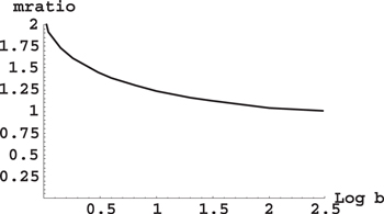
Figure 8. Dependence of the ratio of two values of the scaled projection m of the planet angular momentum on the interstellar axis, mmax/m( ), versus the decimal logarithm of the ratio of the stellar masses b. The value mmax corresponds to the crossing of the energy term, where the planetary motion is stable, with the energy term, where the planetary motion is unstable. The scaled coordinate w = D1, at which
  is calculated, was defined before Figure 6 and in the caption to Figure 6.
Download figure:
Standard image High-resolution imageThe average (over one revolution) interstellar distance is  = p/
= p/ , where
  is the eccentricity and p is the semi-latus rectum (which is the so-called harmonic average p = (1/R
 )/2). The ratio
  /R
/R , where R
 = p/(1+
  ), is
), is

So, the above condition of the stability of the conic-helical planetary orbit close to the star of the smaller mass, m /
/![$m({{D}_{1}})\gt \ {{[\langle R\rangle /{{R}_{{\rm min} }}]}^{1/2}}$](https://content.cld.iop.org/journals/0004-637X/804/2/106/revision1/apj511242ieqn157.gif) , can be reformulated as
, can be reformulated as  (b) where the critical value of the eccentricity
  (b) is

Figure 9 shows the dependence of the critical value of the eccentricity  on the decimal logarithm of the ratio of the stellar masses b. It is seen that in the range 1 < b < 10, corresponding to the overwhelming majority of binary stars, the critical value of the eccentricity is between 0.4 and 0.9. For most of those binary starts, the eccentricity is smaller than the critical value, so that the conic-helical planetary orbit would be stable even if it is close to the star of the smaller mass. (Remember that the conic-helical planetary orbit close to the star of the larger mass is stable for any eccentricity of the stars' orbit.)
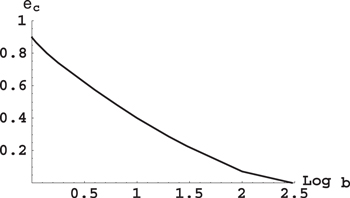
Figure 9. Dependence of the critical value of the eccentricity  on the decimal logarithm of the ratio of the stellar masses b.
Download figure:
Standard image High-resolution imageLet us consider, as an example, the Kepler-16 binary system. According to Doyle et al. (2011), the masses of the two stars are 0.6897 and 0.20255, respectively, in units of the mass of the Sun. So, the ratio of the star masses is b = 3.4. The semimajor axis of the stars' orbit is a = 0.22431 AU, while the eccentricity is  = 0.15944. So, the average interstellar separation is
  = p/
= p/ = 0.22144 AU.
If a planet in the conic-helical orbit was close to the star of the smaller mass, then the distance from the star of the smaller mass to the average orbital plane of the planet would be equal to or smaller than  (3.4)
(3.4) = 0.0077
  = 0.0017 AU. The average radius of the planetary orbit would be equal to or smaller than v(0.0077)
 = 0.029 AU. At b = 3.4, the critical value of the eccentricity
  (3.4) = 0.606. Because the actual eccentricity of the stars' orbit is 0.15944, then the conic-helical planetary orbit would be stable.
If a planet in the conic-helical orbit was close to the star of the larger mass, then the distance from the star of the larger mass to the average orbital plane of the planet would be equal to or smaller than  (3.4)
(3.4) = 0.00216
  = 0.00048 AU. The average radius of the planetary orbit would be equal to or smaller than v(1 − 0.00216)
 = 0.044 AU. The conic-helical planetary orbit would be stable because its stability close to the star of the larger mass is not affected by any value of the eccentricity of the stars' orbit.
4. DETECTION
Exoplanets can be detected photometrically if they are transitable (i.e., if the projections of the planet and the adjacent start on the plane of the sky coincide once in a while). For example, a number of circumbinary planets were detected due to their transitability (see, e.g., Martin & Triaud 2015 and references therein). It turns out that planets in conic-helical orbits at binary stars are highly transitable—meaning that they are transitable for the overwhelming majority of inclinations of the plane of the stars' orbits.
Indeed, for such a planet to be transitable it is sufficient that the inclination I of the stars' orbits exceeds a generally small angle (denoted here as  ) between the average plane of the planetary orbit and the line connecting the planet with the nearest star in the binary. For the planet near the star of the smaller mass, we denote as
  the maximum of all possible angles
  for configurations where the ratio of the orbital frequencies
  of the rapid (the planet) and slow (the binary) subsystems is equal to or exceeds 10—that is, for configurations where the separation into the rapid and slow subsystem is valid. Similarly, for the planet near the star of the larger mass, we denote as
  the maximum of all possible angles
  for configurations where the ratio of the orbital frequencies
  of the rapid (the planet) and slow (the binary) subsystems is equal to or exceeds 10.
Figures 10 and 11 show the dependence of the maximum angles  and
and  , respectively, versus the decimal logarithm of the ratio b of the stellar masses. It is seen that
  ° for all realistic values of b. As for
  , it does not exceed 6° for the ratio of the stellar masses 1 < b < 10 (i.e., for the range corresponding to practically all known binaries). Remember, for configurations where
  , the corresponding curves in Figures 10 and 11 would be located very significantly below the curves
  (b) and
  (b).
(b).
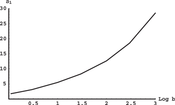
Figure 10. Maximum  of all possible angles α (in degrees), for configurations where the ratio of the orbital frequencies Ω/ω of the rapid (planet) and slow (binary) subsystems is equal to or exceeds 10, versus the decimal logarithm of the ratio of the stellar masses b. Here α is the angle between the average plane of the planetary orbit and the line connecting the planet with the nearest star in the binary, which here is the star of the smaller mass.
Download figure:
Standard image High-resolution image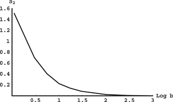
Figure 11. Maximum  of all possible angles α (in degrees), for configurations where the ratio of the orbital frequencies Ω/ω of the rapid (planet) and slow (binary) subsystems is equal to or exceeds 10, versus the decimal logarithm of the ratio of the stellar masses b. Here α is the angle between the average plane of the planetary orbit and the line connecting the planet with the nearest star in the binary, which here is the star of the larger mass.
Download figure:
Standard image High-resolution imageThus, the transitability condition I >  is easily fulfilled for the overwhelming majority of the inclinations of the stars' orbits. This means that conic-helical planetary orbits at binary stars can be detected photometrically. For example, for a Kepler-16 binary star system having the ratio of the stellar masses b = 3.4, the inclination of the star orbits is I = 90.34 degrees (Doyle et al. 2011), so that a conic-helical planetary orbit would be transitable regardless of whether the planetary orbit is close to the star of the smaller or larger mass.
In the future, when the progress of gravitational wave detectors enables the detection of gravitational waves from binary stars, the presence of a planet in a conic-helical orbit could also be revealed by the noticeably enhanced gravitational radiation from the binary star system—for a subset of conic-helical orbits as described in the following. At the first glance, it might seem impossible that the presence of a planet could noticeably enhance the total gravitation radiation from the system: the power P of the gravitational radiation is proportional to the square of the mass, so that due to a small ratio of the masses of the planet and the stars, the additional gravitational radiation due the presence of the planet might seem miniscule. However, the quantity P is also proportional to the 6th power of the orbital frequency (i.e., the dependence of the orbital frequency is much stronger than the dependence on the mass). Therefore, since the orbital frequency of the planet in a conic-helical orbit is much greater than the orbital frequency of the stars in the binary, the power  of the gravitational radiation due to the planet can be comparable or even exceed the power
  of the gravitational radiation due to the stars, as shown below.
Indeed, for two bodies orbiting one another, the power P of the gravitational radiation (i.e., the energy loss per unit time) is the following (see, e.g., Landau & Lifshitz 1971)

where m , f, and R are the reduced mass, the orbital frequency, and the separation; the coefficient a depends on the shape of the orbit. Therefore, the ratio
  /
/ can be estimated as

where

In the notations used in our paper, Q can be represented as

or in the scaled notations

where r[w, b] is the ratio of the orbital frequencies of the planet and the stars given by Equation (41).
From Equation (55), it is seen that the power  gravitational radiation due to the planet can be comparable to the power
  of the gravitational radiation due to the stars if Q is sufficiently large, namely Q
  /m
/m . The quantity Q dramatically increases with the decrease of the relative distance of the plane of the average planetary orbit to the closest star in the binary. We denote by
  the scaled distance of the plane of the average planetary orbit to the star of the smaller mass in the binary, such that at this distance the quantity Q reaches 1000 and exceeds 1000 at smaller distances (the superscript gw stands for gravitational wave). The threshold of 1000 is chosen as an example based on the ratio of masses of the Sun and the Jupiter (there are planets lighter than the Jupiter, but there are also stars lighter than the Sun). Similarly, we denote by
  the scaled distance of the plane of the average planetary orbit to the star of the larger mass in the binary, such that at this distance the quantity Q reaches 1000 and exceeds 1000 at smaller distances.
Figures 12 and 13 shows the dependence of the scaled distances  and
and  , respectively, versus the decimal logarithm of the ratio b of the stellar masses. It is seen that the most favorable situation for the power of the gravitational radiation due to the planet to be comparable to the power of the gravitational radiation due to the stars is when the ratio b of the stellar masses is close to unity.
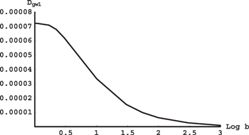
Figure 12. Scaled distances Dgw1 versus the decimal logarithm of the ratio of the stellar masses b. Here Dgw1 is the scaled distance of the plane of the average planetary orbit to the star of the smaller mass in the binary, such that at this distance the power of the gravitational radiation due to the planet is comparable to the power of the gravitational radiation due to the stars (see details in the text).
Download figure:
Standard image High-resolution image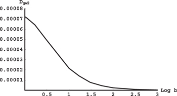
Figure 13. Scaled distances Dgw2 vs. the decimal logarithm of the ratio of the stellar masses b. Here Dgw2 is the scaled distance of the plane of the average planetary orbit to the star of the larger mass in the binary, such that at this distance the power of the gravitational radiation due to the planet is comparable to the power of the gravitational radiation due to the stars (see details in the text).
Download figure:
Standard image High-resolution image
5. CONCLUSIONS
We presented a new type of stable planetary orbits in the OBSS: conic-helical orbits. Namely, the planetary trajectory is a helix on the surface of a cone, whose axis coincides with the interstellar axis. We identified the ranges of parameters where the planetary motion represents a rapid subsystem, while the stellar motion represents a slow subsystem.
We considered the effect of the stars' rotation on the stability of the conic-helical orbits of the planet. We showed that in the above ranges of parameters the rotation of the two stars does not affect the stability of the planetary conic-helical orbit.
We also studied the effect of the eccentricity of the stars' orbits on the stability of the conic-helical orbits of the planet. We demonstrated that even for the eccentric stars' orbits, no matter how high the eccentricity, the conic-helical planetary motion remains stable if the center of symmetry of the helix is relatively close to the star of the larger mass. We also showed that if the center of symmetry of the conic-helical planetary orbit is relatively close to the star of the smaller mass, a sufficiently large eccentricity of stars' orbits can switch the planetary motion to the unstable mode and the planet would then escape the system. More precisely, we demonstrated that for a given eccentricity  of the stellar orbits, the instability would occur if the ratio of the stellar masses b =
  '/
'/ exceeds some critical value
  , the function
  being presented graphically in the present paper.
Finally, we showed that planets in conic-helical orbits at binary stars are transitable for the overwhelming majority of inclinations of the plane of the stars orbits. This means that conic-helical planetary orbits at binary stars can be detected photometrically.
We used an example of Kepler-16 binary stars to provide illustrative numerical data on the possible parameters and the stability of the conic-helical planetary orbits. We also demonstrated that such planetary orbits at Kepler-16 would be transitable.
Then for the general case we also showed that the power of the gravitational radiation due to this planet can be comparable or even exceed the power of the gravitational radiation due to the stars in the binary. This means that in the future, with the progress of gravitational wave detectors, the presence of a planet in a conic-helical orbit could also be revealed by the noticeably enhanced gravitational radiation from the binary star system.