


ABSTRACT
The 1.5 Seyfert galaxy NGC 3516 presents a strong time variability in X-rays. We re-analyzed the nine observations performed in 2006 October by XMM-Newton and Chandra in the 0.3 to 10 keV energy band. An acceptable model was found for the XMM-Newton data fitting the EPIC-PN and RGS spectra simultaneously; later, this model was successfully applied to the contemporary Chandra high-resolution data. The model consists of a continuum emission component (power law + blackbody) absorbed by four ionized components (warm absorbers), and 10 narrow emission lines. Three absorbing components are warm, producing features only in the soft X-ray band. The fourth ionization component produces Fe xxv and Fe xxvi in the hard-energy band. We study the time response of the absorbing components to the well-detected changes in the X-ray luminosity of this source and find that the two components with the lower ionization state show clear opacity changes consistent with gas close to photoionization equilibrium. These changes are supported by the models and by differences in the spectral features among the nine observations. On the other hand, the two components with higher ionization state do not seem to respond to continuum variations. The response time of the ionized absorbers allows us to constrain their electron density and location. We find that one component (with intermediate ionization) must be located within the obscuring torus at a distance 2.7 × 1017 cm from the central engine. This outflowing component likely originated in the accretion disk. The three remaining components are at distances larger than 1016–1017 cm. Two of the absorbing components in the soft X-rays have similar outflow velocities and locations. These components may be in pressure equilibrium, forming a multi-phase medium, if the gas has metallicity larger than the solar one (≳ 5 Z☉). We also search for variations in the covering factor of the ionized absorbers (although partial covering is not required in our models). We find no correlation between the change in covering factor and the flux of the source. This, in connection with the observed variability of the ionized absorbers, suggests that the changes in flux are not produced by this material. If the variations are indeed produced by obscuring clumps of gas, these must be located much closer in to the central source.
Export citation and abstract BibTeX RIS
1. INTRODUCTION
In ∼50% of Type 1 active galactic nuclei (AGNs; e.g., George et al. 1998; Piconcelli et al. 2005), absorption lines are detected in the far-UV and the soft X-ray spectral ranges (Mathur et al. 1995, 1997). These lines, which are blueshifted, are generated by several ionized species. Nearly 100 features are produced in these media with outflow velocities of the order of a few hundred to thousand km s−1 (Crenshaw et al. 2003; Krongold et al. 2003). The location of this absorbing material, referred to as the warm absorber (WA; Halpern 1984), remains uncertain. Suggestions range from the accretion disk itself (Elvis 2000; Krongold et al. 2005a, 2007, 2010; Longinotti et al. 2013) to the obscuring torus (Blustin et al. 2005) and the narrow-line region (e.g., Ricci et al. 2010). There are several models that attempt to explain the distribution and physical conditions of the absorbing gas. One of them proposes that different WA phases can coexist in pressure equilibrium, a multiphase medium (Krongold et al. 2003, 2005b; Cardaci et al. 2009). Another one suggests that the material, also in pressure equilibrium, is distributed with a radial stratification (Różańska et al. 2006). Most X-ray analysis have been based on photoionization models (e.g., Netzer et al. 2003; McKernan et al. 2007; Andrade-Velázquez et al. 2010; Longinotti et al. 2010), where the properties of the absorbing gas are described in terms of the hydrogen equivalent column density and its ionization state. These studies have yielded WA multiphase winds with equivalent column density values NH ∼ 1021 − 23 cm−2. In these kinds of models, the ionization state of the WA components is characterized by the ionization parameter (here defined as U = Q/(4πR2nHc), where Q is the rate of 0.013–100 keV photons produced in the source, R the distance between the black hole and the accretion disk system to WA location, nH the hydrogen number density and c the light speed). As noted by Nicastro et al. (1999) and Krongold et al. (2007), there is a degeneracy in this formula, as only the product neR2 can be inferred from observables. However, time variability analysis solves this problem: by measuring the response time of the absorber to variations in the impinging continuum, the density nH can be estimated (Nicastro et al. 1999) and therefore the distance from the source to the ionized absorber can be constrained (see also Krolik & Kriss 1995; Reynolds et al. 1995; Krongold et al. 2007, 2010).
Studying the properties of the absorbing material is of great importance, as it has been suggested that these outflows can play an important role in galaxy evolution. If the outflowing material is a significant fraction of the accreted mass, the outflows can provide the feedback proposed by the cosmological models (Di Matteo et al. 2005; Hopkins et al. 2006).
1.1. Seyfert 1.5 Galaxy NGC 3516
NGC 3516 is a Seyfert 1.5 galaxy (Véron-Cetty & Véron 2006) at z = 0.00886 (Keel 1996) that presents an extreme X-ray flux variability (Edelson et al. 2000; Netzer et al. 2002; Turner et al. 2008; Markowitz et al. 2008). NGC 3516 is also extremely variable in optical and UV emission (see as examples Voit et al. 1987; Walter et al. 1990; Crenshaw et al. 1998; Goad et al. 1999; Edelson & Nandra 1999; Maoz et al. 2002; Kraemer et al. 2002).
The source has been observed in X-rays from 1979 (Maccacaro et al. 1987) to 2009 (Turner et al. 2011) with all the X-ray observatories (Kolman et al. 1993; Nandra & Pounds 1994; Morse et al. 1995; Kriss et al. 1996; Edelson & Nandra 1999; Costantini et al. 2000; Guainazzi et al. 2001; George et al. 2002; Turner et al. 2008, 2011). NGC 3516 presents a complex spectrum: in the soft X-ray range (0.3–2 keV), the spectrum shows the so-called soft excess, several absorption features attributed to the presence of warm absorbers and few emission lines (Costantini et al. 2000; Guainazzi et al. 2001; George et al. 2002; Turner et al. 2005, 2008; Mehdipour et al. 2010). In the hard band (2–200 keV), it presents the fluorescence iron emission line Kα and two absorption lines by Fe xxv and Fe xxvi. To fit the hard band X-ray continuum of this source, Turner et al. (2005) fitted a power law, finding a photon index Γ ∼ 2 in the 10–200 keV regime. Also, Markowitz et al. (2008) fitted an absorbed power law with Γ = 2 over the 0.3–76 keV range. Recently, Mehdipour et al. (2010) reported a significant change in the slope of the power law among the 2006 XMM-Newton observations: Γ varied from 1.70 ± 0.2 to 1.85 ± 0.2, in addition to significant changes in the 0.2 to 10 keV range flux.
To model the soft excess emission Markowitz et al. (2008) added a second power law, with the same photon index as the primary power law but not obscured by any absorber. Mehdipour et al. (2010) added a modified blackbody component which describes the spectrum of a blackbody reprocessed by coherent Compton scattering. The best-fit temperature varied from 186 ± 3 eV to 211 ± 4 eV. We note that the soft excess physical interpretation is still an issue (see Ricci et al. 2010).
1.2. Previous Analysis of the Ionized Absorber in NGC 3516
The complex absorption in NGC 3516 soft X-ray band was detected by two strong absorption features at 0.74 and 0.87 keV with the ROSAT (Mathur et al. 1997) and ASCA X-ray telescopes (Kriss et al. 1996). These features were originally interpreted as absorbing K edges due to O vii and O viii bound–free transitions. More recently, a few high ionization absorption components producing both absorption lines and edges have been detected in high-resolution spectra. Turner et al. (2005) reported three ionization states: (1) a "cool" absorber with a column density NH ∼ 6 × 1021 cm−2 and an outflow velocity vout = −200 km s−1 (all the outflow velocities in this work were fixed to a given value), associated with the "UV absorber" found by Kraemer et al. (2002); (2) a "high ionization" absorber with NH ∼ 1022 cm−2 and a fixed vout = −1100 km s−1; and (3) a "heavy" absorber with NH ∼ 1023 cm−2 and vout = −1100 km s−1 that covers only 50% of the continuum source. Later on, Turner et al. (2008) discovered a fourth absorbing component with an even higher ionization state through the positive detection of H-like and He-like features of Fe xxv and xxvi. This component, only detectable in the hard X-ray band, has NH ∼ 1023 cm−2 and vout ∼ −1000 km s−1. Turner et al. (2008) interpreted the flux variations in the X-ray band as the result of variations in the covering fraction of the "heavy absorber."
Using low-resolution Suzaku data, Markowitz et al. (2006) found two absorbing components: a "primary absorber" with properties consistent with the "heavy" absorber reported by Turner et al. (2008; although with a covering fraction of 96–100%) and a mildly ionized medium, consistent with the "UV absorber." Mehdipour et al. (2010) analyzed the XMM-Newton data of the source. They detected the same three absorbing components as Turner et al. (2008), but they reported that partial covering is not required by the data for the heavy absorber. If these authors impose a partial absorber in their models, they further find that variations in the covering fraction are not consistent with the data (in contrast to the results by Turner et al. 2008).
Finally, Holczer & Behar (2012) found a kinematic structure in the absorber, consisting of four different outflow components intrinsic to NGC 3516: (1) vout = −350 ± 100 km s−1, (2) vout = −1500 ± 150 km s−1, (3) vout = −2600 ± 200 km s−1, and (4) vout = −4000 ± 400 km s−1. Holczer & Behar (2012) analyzed the Chandra high-resolution spectra obtained in 2001 and 2006. They detect variability in this structure, noting that the high velocity components are only present in the 2006 observations. They further report that the covering factor plays a minor role in the absorption lines.
In the UV band, Kraemer et al. (2002) have reported eight different kinematic absorbing components. Using data obtained by the GHRS (Goddard High Resolution Spectrograph) on board the Hubble Space Telescope (HST), these authors detected four of these components through Lyα, CIV, and NV absorption lines with radial velocities of −376, −183, and −36 km s−1 (where the last system is comprised by a blend of two different kinematic components). Later on, the other four kinematic components were detected with the Space Telescope Imaging Spectrograph (STIS) on board the HST. These components present radial velocities of −692, −837, −994, and −1372 km s−1. These authors suggest that the emergence of the new components is the result of variations of ionized gas in response to changes in the ionizing continuum.
1.3. X-Ray Variability on NGC 3516
As it has been reported NGC 3516 presents strong flux variations in time, from the optical–UV to the X-rays (see for example Koratkar et al. 1996 and Kraemer et al. 2002). The source presents extreme X-ray flux variations by a factor of five on timescales of hours (Turner et al. 2008), and by a factor of 50 in timescales of years (Netzer et al. 2002). These variations are often associated with spectral changes (e.g., Netzer et al. 2002; Turner et al. 2008 and references therein) not only in the energy flux, but also with evidence of spectral feature variability (Mathur et al. 1997; Netzer et al. 2002; Turner et al. 2008; Holczer & Behar 2012). To understand the nature of the variability, some scenarios invoking obscuration have been proposed. Costantini et al. (2000) suggested neutral clouds that hide the central source (using Beppo SAX telescope spectra), and Markowitz et al. (2008; with Suzaku spectra) proposed a model in which flux variations could be explained by the presence of discrete blobs or filaments located within few light years of the black hole, traversing the line of sight during the observation time. Turner et al. (2008) suggested a simple explanation were that only parameter varying among observations (and producing both the flux and spectral variations) is the covering factor of the heavy absorber phase.
Other interpretations suggest that rather, the variations might be intrinsic to the source. Mehdipour et al. (2010) arrived at this conclusion using 2006 XMM-Newton spectra.
However, in a most recent X-ray NGC 3516 analysis, using 2009 Suzaku X-ray observations, Turner et al. (2011) claim an absence of reverberation signals. This led them to conclude that intrinsic continuum variability is not possible. They suggested that the variability can be a consequence of Compton-thick clumps of gas in the line of slight.
In this paper, we present the analysis of all 2006 X-ray observations available in the XMM-Newton Science Archive (XSA) and Chandra Data Archive (CDA) of NGC 3516. We study both high- and low-resolution spectra to cover the range between 0.3 keV to 10 keV. We first present the analysis over individual spectra to characterize the spectral components and then study the time variability of the absorber among observations. In our analysis, we find variations in two of the ionized absorbers in response to continuum variations.
Section 2 describes the X-ray observations and the data reduction. In Section 3, we present 2006 X-ray data analysis and the best model for XMM-Newton data; we also describe the Chandra analysis. Section 4 contains our results, including the time variability behavior and a physical scenario proposed to explain the X-ray proprieties and the flux variability of NGC 3516. We discuss our results in Section 5. Finally, in Section 6, we present the conclusions.
2. X-RAY OBSERVATIONS AND DATA REDUCTION
X-ray observations of NGC 3516 were obtained with the XMM-Newton (Jansen et al. 2001) and Chandra X-ray observatories (Weisskopf et al. 2000) in 2006 October. The log of observations is presented in Tables 1 and 2 for the XMM-Newton and Chandra X-ray observatories, respectively. In the following we describe the data properties and reduction process.
Table 1. Observation Mean Count Rate and Exposure Time of XMM-Newton Observations taken in 2006 October
| Observation | ObsID | Obs. Date | Exposure Time | Mean Count Rate | ||
|---|---|---|---|---|---|---|
| (Year/Month/Day) | (s) | (counts s−1) ±σ | ||||
| PN | RGS | PN | RGS | |||
| 1 XMM [1x] | 0401210401 | 2006-10-06 | 36142 | 51558 | 30.80 | 0.90 |
| 2 XMM [2x] | 0401210501 | 2006-10-08 | 48031 | 68752 | 28.60 | 0.84 |
| 3 XMM [5x] | 0401210601 | 2006-10-10 | 47534 | 68203 | 15.61 | 0.49 |
| 4 XMM [8x] | 0401211001 | 2006-10-12 | 47608 | 67813 | 27.45 | 0.96 |
Download table as: ASCIITypeset image
Table 2. Observation Count Rate and Exposure Time of Chandra Observations taken in 2006 October
| Observation | ObsID | Obs. Date | Exposure time | Mean Count Rate | ||
|---|---|---|---|---|---|---|
| (Year/Month/Day) | (s) | (counts s−1) ±σ | ||||
| MEG | HEG | MEG | HEG | |||
| 1 CXO [3c] | 8452 | 2006-10-09 | 19832 | 19832 | 0.62 | 0.32 |
| 2 CXO [4c] | 7282 | 2006-10-10 | 41410 | 41410 | 0.41 | 0.23 |
| 3 CXO [6c] | 8451 | 2006-10-11 | 47360 | 47360 | 0.74 | 0.38 |
| 4 CXO [7c] | 8450 | 2006-10-12 | 38505 | 38505 | 0.79 | 0.39 |
| 5 CXO [9c] | 7281 | 2006-10-14 | 42443 | 42443 | 0.40 | 0.23 |
Download table as: ASCIITypeset image
2.1. XMM-Newton Observatory Data
We studied all the NGC 3516 XMM-Newton X-ray spectra from the RGS (Reflection Grating Spectrometer) and the EPIC-PN (European Photon Imaging Camera). The observations were performed between 2006 October 6 and 12.
The RGS data were processed with the standard pipeline of Science Analysis System (SAS) v8.0.1 (Gabriel et al. 2004). We produced source and background spectra, as well as response matrices for the RGS data with the rgsproc task. The RGS spectra were grouped into two channels per bin. We considered the wavelength range from 8 to 38 Å [0.33–1.55 keV], which covers most of the soft X-ray band.
EPIC-PN spectra were also generated using SAS. First, intervals of flaring particle background were selected in order to clean the event list using the method presented in Piconcelli et al. (2004). The spectra were extracted from a circle with center on the observed position of NGC 3516 and radius ∼40'' in all observations. The background spectra were obtained from a circular region with similar radius in the same chip of the source. No sign of pile-up was detected in any of the observations as reported before by Turner et al. (2008) and Mehdipour et al. (2010). The source and background spectra were generated with the evselect task. Then, the redistribution matrix and the ancillary files were created with the rmfgen and the arfgen tasks, respectively. The spectra were grouped to a minimum of 20 counts per bin in order to be able to use χ2 statistics. We selected the interval from 0.3 keV to 10 keV that includes the soft and hard X-ray bands. In Table 1, the net count rate and the exposure time for each ObsID and detector of the XMM-Newton observations of NGC 3516 are shown.
2.2. Chandra X-Ray Observatory Data
The Chandra X-ray observations were performed from 2006 October 9 to October 14 using the High Energy Transmission Grating (HETGS) with the ACIS-S (Advanced CCD Imaging Spectrometer). The HETGS (Canizares et al. 2000) contains two grating assemblies, the Medium-Energy Grating (MEG) and High-Energy Grating (HEG). We extracted spectra from both gratings using the Chandra Interactive Analysis of Observations software (CIAO v.3.4, Fruscione et al. 2006; we followed the standard pipeline processes). Negative and positive first-order spectra and their response matrices were obtained and co-added. The spectra were grouped into two channels per bin. The count rates and the exposure time in the MEG and HEG spectra are given in Table 2.
3. DATA ANALYSIS
3.1. Time Variability
The 2006 X-ray observations of NGC 3516 were performed with almost continuous time coverage (with XMM-Newton and/or Chandra) on a timescale of nine days (see Tables 1 and 2). We have numbered the observations in sequential order according to the date of observation, and further included an x suffix if performed by XMM-Newton or a c suffix if obtained with Chandra.
There is strong flux variability among different observations with the same observatory (compare count rates for observations with the same observatory/instrument in Tables 1 and 2) and within single observations. A detailed light curve of the nine observations can be observed in Figures 1 and 2 of Turner et al. (2008). In this paper, we study the temporal evolution of the absorbing components in response to these flux changes.
3.2. XMM-Newton Spectral Analysis
We performed the analysis of the XMM-Newton observations using simultaneously both the EPIC-PN and RGS data sets. All spectra were analyzed with the Sherpa (Freeman et al. 2001) package included in the CIAO software. Throughout the paper, we attenuate all models with an equivalent H column density NH = 3.23 × 1020 cm−2 (Dickey & Lockman 1990) to account for the Galactic absorption in the line of sight toward NGC 3516.
3.2.1. Analysis in the X-Ray Hard Energy Band
First, we modeled the NGC 3516 EPIC-PN spectra in the 2.5–10 keV band. We fit the data using a redshifted power law model plus a Gaussian to account for the Fe-Kα emission line reported by Turner et al. (2008) and Mehdipour et al. (2010). This model presents strong negative residuals around 7 keV, confirming the two significant absorption lines reported by Turner et al. (2008) and Mehdipour et al. (2010), corresponding to Fe K transitions of Fe xxv and Fe xxvi. These features were modeled with Gaussians at this initial stage (although a self consistent photoionization model was applied to this absorption system later on). Table 3 lists the best-fit parameters for each observation. The model is statistically acceptable for all observations (Table 3).
Table 3. Hard Band Fit: 2.5–10 keV Energy Band
| Obs | Power Law | Fe–Kα | Fe xxv | Fe xxvi | Statistics | |
|---|---|---|---|---|---|---|
| Γ | Norma | Pos(keV) | Pos(keV) | Pos(keV) | χred/dof | |
| σ (keV) | σ (keV) | σ (keV) | (2.5–10 keV) | |||
| Normb | Normb | Normb | ||||
| 1x | 1.64 ± 0.02 | 1.22 ± 0.02 |  |
6.73 ± 0.03 | 7.04 ± 0.02 | 0.79/1364 |
 |
0.04 ± 0.04 | 0.05 ± 0.04 | ||||
 |
 |
−1.58 ± 0.03 | ||||
| 2x | 1.59 ± 0.02 | 0.99 ± 0.02 | 6.39 ± 0.02 | 6.703 ± 0.019 | 7.05 ± 0.02 | 1.08/1411 |
| 0.12 ± 0.02 | 0.03 ± 0.04 | 0.05 ± 0.04 | ||||
 |
−1.15 ± 0.23 | −1.38 ± 0.23 | ||||
| 5x | 1.45 ± 0.02 | 0.65 ± 0.02 | 6.38 ± 0.02 | 6.75 ± 0.02 | 7.08 ± 0.02 | 1.17/1357 |
| 0.13 ± 0.02 | 0.02 ± 0.04 | 0.03 ± 0.03 | ||||
 |
−1.06 ± 0.21 | −1.16 ± 0.22 | ||||
| 8x | 1.54 ± 0.02 | 0.95 ± 0.02 | 6.41 ± 0.02 | 6.78 ± 0.02 |  |
0.79/1483 |
| 0.09 ± 0.02 | 0.04 ± 0.03 | 0.05 ± 0.03 | ||||
 |
−1.84 ± 0.31 | −1.86 ± 0.32 | ||||
Notes. a In 10−2 photons keV−1 cm−2 s−1 at 1 keV. b In 10−5 photons cm−2 s−1 in the line.
Download table as: ASCIITypeset image
Table 4. Whole Band Fit: 0.3–10 keV
| Obs | Power Law | Blackbody | Statistics | |||
|---|---|---|---|---|---|---|
| Γ | kT (keV) | χred/dof | ||||
| Norma | Normb | (0.3, 10 keV) | ||||
| 1x | 1.31 ± 0.02 | 0.08 ± 0.02 | 4.5/4534 | |||
| 0.78 ± 0.02 | 5.92 ± 0.05 | |||||
| 2x | 1.30 ± 0.02 | 0.09 ± 0.02 | 5.2/4581 | |||
| 0.66 ± 0.02 | 5.85 ± 0.04 | |||||
| 5x | 1.05 ± 0.02 | 0.09 ± 0.02 | 4.2/4527 | |||
| 0.36 ± 0.02 | 2.99 ± 0.03 | |||||
| 8x | 1.21 ± 0.02 | 0.09 ± 0.02 | 5.2/4655 | |||
| 0.61 ± 0.02 | 6.38 ± 0.04 | |||||
Notes.
a In 10−2 photons keV−1 cm−2 s−1 in al 1 keV.
b In 10−4  units, L39 is the source luminosity in units of 1039 erg s−1 and D10 is the distance to the source in units of 10 kpc.
Download table as: ASCIITypeset image
3.2.2. X-Ray Broadband Analysis
We fit the EPIC-PN and RGS simultaneously, extrapolating the fit in the hard band to the entire spectrum [0.3–10 keV]. A soft X-ray excess is evident in the residuals. We fit this emission feature with a blackbody. Initially, we left the temperature of the blackbody free to vary independently among observations. However, since in all XMM-Newton observations the kT value is always around 0.1 keV (see Table 4), this parameter was free to vary but constrained to have the same value in all observations (the temperature of the blackbody was linked to a single best-fit value among the all observations). The normalization was fit independently in each observation.
This model presents strong residuals in the soft band typical of ionized absorption due to the well-known warm absorber in this source.
3.2.3. Modeling the Ionized Absorber in NGC 3516
There have been several studies of the warm absorbers in NGC 3516 reporting a different number of ionization components. In order to establish the presence of each component, we decided to add one absorber component at a time in our models. This allows us to test statistically its presence and also to inspect visually its contribution to the overall opacity.
The PHASE code (Krongold et al. 2003) was used to fit the warm absorbers (WA). The model has four free parameters: (1) the ionization parameter U (U = Q/(4πR2nHc))6; (2) the equivalent hydrogen column density NH; (3) the outflow velocity vz; and (4) the internal micro-turbulence velocity vturb. The spectral energy distribution (SED) of the source, also required in the models, was obtained from NED (NASA/IPAC Extragalactic Database) between the radio and the UV regimes and complemented with our fits to the X-ray band. The SED is shown in Figure 1.
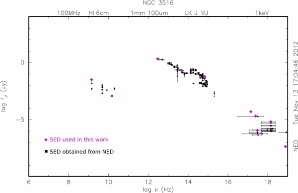
Figure 1. Spectral energy distribution of NGC 3516. The black dots are reported by NED, while in this work, we derived the fuchsia points values.
Download figure:
Standard image High-resolution imageWe note that the estimated errors in the outflow velocity of the absorber are too small, in general, smaller than the resolution of the detectors. For this reason, throughout the paper we consider a conservative error in this parameter as half the minimum spectral resolution of the RGS (700 km s−1 in 15 Å): Δvout = 350 km s−1. We prefer this conservative value given that the fits to the data include several blended absorption lines from different charge states as well as the blend of several velocity components present in absorption.
Our first model (Model A) consists of a single ionization component and an F-test confirms its presence with >99.99% confidence level for all observations. This component models absorbing lines produced mainly by O vii, O viii, as well as part of the Fe M-shell unresolved transition array (UTA), among others. The outflow velocity is −532 ± 350 km s−1.
Model B included a second WA absorbing phase. A statistically better fit than Model A is supported by an F-test (>99.99% of significance for all XMM-Newton observations). The second absorber fits absorption lines with a higher level of ionization, mainly Fe L-shell absorption from charge states xvii to xxii, also including absorption by Ne x. The outflow velocity is higher also, −1845 ± 350 km s−1. We note that the two ionized absorption phases had different U and NH values among observations. We will analyze these changes in Section 4.1.
Given that residuals were still present, we further included a third WA phase (Model C). At the beginning, all the parameters were free to vary. However, for each absorbing component, the best-fit value of the outflow velocity vout among the observations was similar, with differences lower than the RGS resolution: 700 km s−1 (in 15 Å). Thus, we left the outflow velocity of each absorber as a free parameter but constrained it to have the same best-fit value in all the observations (we link this parameter in the models for all observations, assuming no acceleration or deceleration in the flow during the total observing time). Given that the best-fit values of the turbulent velocity vturb were also very similar among observations with differences lower than RGS resolution, we performed the same procedure with the turbulent velocity, linking this free parameter to a single value in all data sets. According to an F-test, the third absorber included in model C is statistically required by the data (probability >99.99%). This third absorber is modeling low ionization lines produced by charge states such as Ne v and Ne vi, and a fraction of the Fe M-shell UTA. This component had an outflow velocity best-fit value higher than the other two absorbers, vout = −2425 ± 350 km s−1.
Thus, this final model includes of three absorbing components. The first one consists of a medium level of ionization (hereafter phase MI), the second phase presents high ionization (hereafter phase HI), and the third one is produced by low ionized gas (hereafter phase LI). Tables 5 and 6 summarize the models applied in the four XMM-Newton spectra.
Table 5. Models to Fit NGC 3516 in XMM-Newton Observations
| Model | Power Law | Blackbody | WA Parameters | Statistics | ||||
|---|---|---|---|---|---|---|---|---|
| Γ | Norma | KT | Normb | Phase LI | Phase MI | Phase HI | χred/dof | |
| Obs 1x | ||||||||
| A | 1.69 ± 0.02 | 1.36 ± 0.02 | 0.10 ± 0.02 | 9.18 ± 0.06 | √ | 1.44/4530 | ||
| B | 1.78 ± 0.02 | 1.58 ± 0.04 | 0.10 ± 0.02 |  |
√ | √ | 0.95/4526 | |
| C | 1.81 ± 0.02 | 1.67 ± 0.06 | 0.09 ± 0.02 | 6.47 ± 0.02 | √ | √ | √ | 0.86/4504 |
| Obs 2x | ||||||||
| A | 1.66 ± 0.02 | 1.11 ± 0.02 | 0.10 ± 0.02 |  |
√ | 1.73/4577 | ||
| B | 1.71 ± 0.02 | 1.23 ± 0.02 | 0.10 ± 0.02 | 5.78 ± 0.04 | √ | √ | 1.16/4573 | |
| C | 1.74 ± 0.05 | 1.31 ± 0.09 | 0.09 ± 0.02 | 6.50 ± 0.40 | √ | √ | √ | 1.04/4557 |
| Obs 5x | ||||||||
| A | 1.47 ± 0.02 | 0.68 ± 0.02 | 0.10 ± 0.02 |  |
√ | 1.23/4523 | ||
| B | 1.54 ± 0.02 | 0.79 ± 0.02 | 0.10 ± 0.02 |  |
√ | √ | 0.98/4519 | |
| C | 1.61 ± 0.02 | 0.89 ± 0.02 | 0.09 ± 0.02 | 4.39 ± 0.04 | √ | √ | √ | 0.88/4503 |
| Obs 8x | ||||||||
| A | 1.63 ± 0.02 | 1.13 ± 0.02 | 0.10 ± 0.02 | 8.09 ± 0.05 | √ | 1.74/4649 | ||
| B | 1.70 ± 0.02 | 1.28 ± 0.02 | 0.09 ± 0.02 |  |
√ | √ | 1.12/4645 | |
| C | 1.75 ± 0.05 | 1.4 ± 0.2 | 0.09 ± 0.02 | 7.9 ± 0.4 | √ | √ | √ | 0.97/4629 |
Notes.
a In 10−2 photons keV−1 cm−2 s−1 in at 1 keV.
b In 10−4  units, L39 is the source luminosity in units of 1039 erg s−1 and D10 is the distance to the source in units of 10 kpc.
Download table as: ASCIITypeset image
Table 6. WA Parameters of NGC 3516
| Model C | Phase LI | Phase MI | Phase HI | ||||||
|---|---|---|---|---|---|---|---|---|---|
| logU | logNH | logU | logNH | logU | logNH | ||||
| velz (km s−1) | velturb (km s−1) | velz (km s−1) | velturb (km s−1) | velz (km s−1) | velturb (km s−1) | ||||
| Obs 1x | |||||||||
| A |  |
21.82 ± 0.02 | |||||||
| −888 ± 350 | 286 ± 350 | ||||||||
| B | 0.16 ± 0.02 | 21.65 ± 0.02 |  |
22.07 ± 0.02 | |||||
| −995 ± 350 | 220 ± 350 | −2302 ± 350 | 320 ± 350 | ||||||
| C |  |
21.14 ± 0.02 | 0.38 ± 0.02 | 21.56 ± 0.02 | 1.69 ± 0.02 | 22.25 ± 0.02 | |||
| −2425 ± 350 | 88 ± 350 | −532 ± 350 | 239 ± 350 | −1845 ± 350 | 112 ± 350 | ||||
| Obs 2x | |||||||||
| A | 0.27 ± 0.02 | 21.82 ± 0.02 | |||||||
| −1018 ± 350 | 207 ± 350 | ||||||||
| B | 0.18 ± 0.02 | 21.68 ± 0.02 | 1.95 ± 0.02 | 22.29 ± 0.08 | |||||
| −1082 ± 350 | 195 ± 350 | −1851 ± 350 | 77 ± 350 | ||||||
| C | −0.78 ± 0.05 | 20.98 ± 0.08 | 0.27 ± 0.02 | 21.52 ± 0.09 | 1.68 ± 0.09 | 22.197 ± 0.164 | |||
| => 1x | => 1x | => 1x | => 1x | => 1x | =>1x | ||||
| Obs 5x | |||||||||
| A | 0.215 ± 0.024 | 21.94 ± 0.02 | |||||||
| −1388 ± 350 | 168 ± 350 | ||||||||
| B | 0.12 ± 0.02 | 21.75 ± 0.02 | 1.68 ± 0.02 | 22.22 ± 0.03 | |||||
| −1066 ± 350 | 199 ± 350 | −885 ± 350 | 143 ± 350 | ||||||
| C | −1.22 ± 0.02 | 21.25 ± 0.02 | 0.29 ± 0.02 | 21.62 ± 0.02 | 1.77 ± 0.02 | 22.33 ± 0.14 | |||
| => 1x | => 1x | => 1x | => 1x | => 1x | =>1x | ||||
| Obs 8x | |||||||||
| A | 0.33 ± 0.02 | 21.93 ± 0.02 | |||||||
| −1154 ± 350 | 202 ± 350 | ||||||||
| B | 0.18 ± 0.03 | 21.69 ± 0.02 | 1.77 ± 0.02 | 22.07 ± 0.02 | |||||
| −619 ± 350 | 234.9 ± 350 | −2293 ± 350 | 417 ± 350 | ||||||
| C | −0.78 ± 0.02 | 21.25 ± 0.09 | 0.38 ± 0.02 | 21.512 ± 0.032 | 1.96 ± 0.22 | 22.48 ± 0.22 | |||
| => 1x | => 1x | => 1x | => 1x | => 1x | =>1x | ||||
Notes. In Model C, we referred the vout and vout to the values of observation 1x; however, the final values were fitted taking into account the four XMM-Newton observations.
Download table as: ASCIITypeset image
Although the data does not present strong residuals consistent with additional absorption features, we tested a possible fourth WA component in the soft X-ray RGS data. An F-test does not show a statistical improvement over Model C.
3.2.4. Emission Features in the Spectra
The presence of positive residuals in the spectra, associated with emission lines in the rest frame of the object, is evident in the data. Through a detailed visual inspection we identified nine emission features using ATOMDB version 1.3.1 from the Chandra X-ray Center (http://asc.harvard.edu/atomdb/WebGUIDE/), and modeled them with Gaussian components. The FWHM was fixed to 300 km s−1, given that they are not resolved. We found two emission lines corresponding to Ne transitions (Ne vi and Ne ix), five corresponding to O vii, three of them belonging to the triplet between 21.6–22.1 Å, and two lines of highly ionized Iron (Fe xix and Fe xxi). Table 7 shows the nine emission lines detected in the soft X-ray band for each observation.
Table 7. Emission Lines in the Soft Band of XMM-Newton and Chandra
| Transitiona | Ne ix | Fe xix | O vii | Fe xix | O vii | O vii | O vii | Fe xxi | Ne vi |
|---|---|---|---|---|---|---|---|---|---|
| λ13.69* | λ13.91* | λ17.39* | λ17.86* | λ21.60* | λ21.81* | λ22.10* | λ28.53* | λ28.92* | |
| Wavelength Observed (Å) | |||||||||
| Observation | Energy Fluxb | ||||||||
| 1x | 13.79 ± 0.08 | 14.04 ± 0.04 | 17.73 ± 0.02 | 18.05 ± 0.12 | 21.64 ± 0.02 | 21.93 ± 0.02 | 22.29 ± 0.22 | 28.83 ± 0.03 | 29.19 ± 0.02 |
| 1.4 ± 0.5 | 2.4 ± 0.6 | 1.9 ± 0.05 | 1.9 ± 0.05 | 9.8 ± 3.2 | 3.9 ± ... | 0.9 ± 0.8 | 0.5 ± 0.2 | 2.6 ± 0.7 | |
| 2x | 13.79 ± 0.02 | 14.04 ± 0.02 | 17.67 ± 0.03 | 18.19 ± 0.03 | 21.59 ± 0.02 | 21.89 ± 0.08 | 22.29 ± 0.09 | 28.86 ± 0.02 | 29.18 ± 0.02 |
| 2.4 ± 0.5 | 1.6 ± 0.5 | 0.9 ± 0.4 | 1.2 ± 0.5 | 0.9 ± 0.8 | 1.2 ± 0.9 | 2.9 ± 0.7 | 0.2 ± 0.5 | 2.9 ± 0.7 | |
| 3c | 13.81 ± 0.10 | 14.06 ± 0.02 | 17.67 ± ...c | 18.16 ± 0.72 | 21.6 ± ... | 21.91 ± ... | 22.30 ± ... | O.R.d | O.R. |
| 1.5 ± 0.9 | 2.6 ± 1.3 | 1.5 ± 1.8 | 2.2 ± 2.1 | 0 ± ... | 3.4 ± ... | 3.4 ± ... | |||
| 4c | 13.82 ± 0.04 | 14.06 ± 0.06 | 17.74 ± 0.08 | 18.21 ± ... | 21.59 ± ... | 21.82 ± | 22.31 ± ... | O.R. | O.R. |
| 0.8 ± 0.5 | 1.07 ± 0.7 | 0.7 ± 0.6 | 0.7 ± 0.9 | 1.5 ± ... | 7.7 ± 7.2 | 6.2 ± 5.5 | |||
| 5x | 13.79 ± 0.02 | 14.04 ± 0.02 | 17.65 ± 0.02 | 18.16 ± ... | 21.64 ± | 21.89 ± 0.2 | 22.29 ± 0.02 | 28.82 ± ... | 29.19 ± 0.04 |
| 0.9 ± 0.3 | 2.7 ± 1.2 | 1.2 ± 0.4 | 0.7 ± 0.5 | 8.2 ± 3.3 | 1.6 ± 0.4 | 1.9 ± 0.5 | 0.4 ± 0.6 | 1.2 ± 0.5 | |
| 6c | 13.82 ± 0.04 | 14.06 ± 0.02 | 17.64 ± ... | 18.11 ± 0.10 | 21.62 ± 0.02 | 21.90 ± 0.04 | 22.31 ± ... | O.R. | O.R. |
| 0.9 ± 0.6 | 2.2 ± 0.8 | 0.4 ± 0.4 | 2.6 ± 1.5 | 709 ± 645 | 3.6 ± 2.2 | 4.5 ± 2.6 | |||
| 7c | 13.81 ± ... | 14.05 ± 0.02 | 17.71 ± 0.04 | 18.08 ± ... | N.D.e | 21.92 ± 0.36 | 22.26 ± | O.R. | O.R. |
| 0.6 ± 0.7 | 1.4 ± 0.9 | 2.2 ± 1.4 | 1.02 ± 1.33 | 0 ± ... | 2.2 ± 3.2 | 1.2 ± 6.2 | |||
| 8x | 13.79 ± ... | 14.04 ± | 17.78 ± 0.02 | 18.07 ± 0.15 | 21.62 ± 0.12 | 21.88 ± | 22.31 ± 0.02 | N.D. | 29.21 ± .08 |
| 1.1 ± 1.9 | 0.8 ± 0.9 | 0.6 ± 0.5 | 6.2 ± 4.8 | 123 ± 115 | 2.4 ± 0.6 | 1.99 ± 0.75 | 0 ± ... | 2.2 ± 1.7 | |
| 9c | 13.82 ± 0.2 | 14.07 ± 1.8 | 17.714 ± 0.12 | 18.02 ± 0.7 | N.D. | N.D. | 22.3 ± ... | O.R. | O.R. |
| 0.9 ± 1.3 | 3.6 ± 4.2 | 1.15 ± 1.3 | 1.6 ± 1.5 | 0 ± ... | 0 ± ... | 1.6 ± ... | |||
Notes. a Ion name and transition rest-frame wavelength (Å)*. b In 10−4 photons cm−2 s−1 in the line. c ... means indeterminate. d O.R. means line out of detector range. e N.D. means line not detected.
Download table as: ASCIITypeset image
We stress that not all the emission lines were detected in a significant way in all the observations. However, the fluxes of all lines are consistent with each other among all the observations, with the only exception of the O vii–Kα transition at λ ∼ 21.6 Å. The differences in this transition are probably due to the strong blending of this line with the strong absorption feature produced by the WA. We point out that Mehdipour et al. (2010) only modeled one emission line in the soft X-ray energy band, namely, O vii (f). These authors only include this feature as it is the only one significant in all observations. Nevertheless, in their Figure 6, it is possible to observe residuals coincident with the emission lines identified here. For instance, at wavelengths around λ ∼ 13.8, ∼17.8, ∼18, ∼22.2, and ∼29.2 Å.
Summarizing, our final model consists of Model C (including the three absorbing component in the soft band) plus the fourth absorbing phase (VH) in the hard band, plus the nine emission lines described above. The figures with the final models (including a simultaneous fit to the Chandra and XMM-Newton data; see Section 3.3) are presented in Figures 2–6. Table 8 contains the observed energy flux values for all observations. The flux was integrated in two different energy ranges: in the soft energy band [8–25 Å: 0.49–1.55 keV] and in the hard energy band [1.55–10 keV]. The reported quantities correspond to the intrinsic flux of the source without attenuation by Galactic absorption (see Section 3.2) and the warm absorber components.
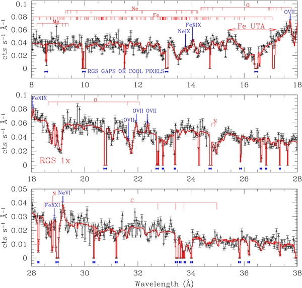
Figure 2. RGS spectrum of observation 1x together with the Model C fit (red) [8–38 Å]. The absorption lines are identified above with the corresponding transition and the main emission lines are marked in blue (top of the panel). The detector gaps the cool pixels of RGS are marked in blue on the bottom of the panel (http://heasarc.gsfc.nasa.gov/docs/xmm/uhb/rgsmultipoint.html).
Download figure:
Standard image High-resolution imageTable 8. Energy Flux [Fhν] of NGC 3516: Soft X-Ray Band and Hard X-Ray Band
| Obs | Soft Band | Hard Band | ||
|---|---|---|---|---|
| Fhνa (8–25 Å: 0.49–1.55 keV) | Fhνa (1.55–10 keV) | |||
| 1x | 1.87 ± 0.05 | 2.59 ± 0.03 | ||
| 2x | 1.69 ± 0.03 | 2.34 ± 0.02 | ||
| 3c | 1.09 ± 0.04 | 2.04 ± 0.03 | ||
| 4c | 0.707 ± 0.019 | 1.58 ± 0.03 | ||
| 5x | 0.88 ± 0.03 | 1.97 ± 0.02 | ||
| 6c | 1.54 ± 0.03 | 2.22 ± 0.05 | ||
| 7c | 1.72 ± 0.03 |  | ||
| 8x | 1.84 ± 0.04 | 2.46 ± 0.03 | ||
| 9c | 0.50 ± 0.02 |  | ||
Download table as: ASCIITypeset image
3.3. Simultaneous XMM-Newton and Chandra Spectral Analysis
Once we had a satisfactory fit with XMM-Newton, we proceeded to model the contemporary Chandra spectra. We fit the Chandra data, applying a model consisting of Model C (including the three ionized absorbers detected in the soft energy band) plus the nine emission lines included in the XMM-Newton fits. Both MEG [2–25 Å: 0.5–6.2 keV] and HEG data [1.6–15 Å: 0.8–7.7 keV] were fitted simultaneously.
All nine observations (including those from XMM-Newton and Chandra) were fitted simultaneously, leaving free to vary independently in each observation the photon index and normalization of the power law and the normalization of the blackbody. The temperature kT [keV] of the blackbody emission was free to vary, but constrained to have a single value in all data. The ionization parameter and the column density of the three absorbing components was also fitted independently among different observations. However, as before, the outflow and turbulent velocities of each phase were free to vary, but linked between the nine observations to give a single best-fit value.
The best-fit parameters of this final model are presented in Table 9. The fits over the high-resolution (RGS) spectra are shown in Figures 2, 3, 4, and 5 for observations 1x, 2x, 5x, and 8x, respectively. The MEG of Chandra data and best-fit models are shown in Figure 6. All statistical results are satisfactory with χred ∼ 1 (Table 9). We note that the values for the ionization parameter and column density on each XMM-Newton observation are consistent within 35% (and within the errors) with those found over the fits excluding the Chandra data (Model C, Section 3.2).
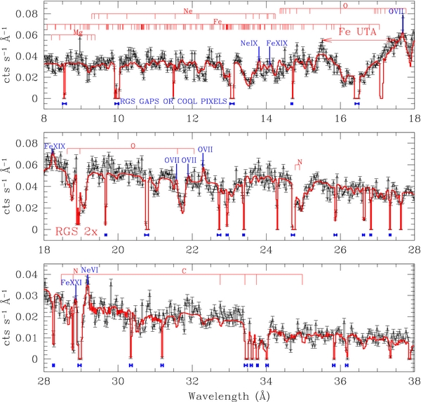
Figure 3. RGS spectrum of observation 2x together with the Model C fit (red) [8–38 Å]. The absorption lines are identified above; the corresponding transition and the main emission lines are marked in blue (top of the panel). The detector gaps or the cool pixels of RGS are marked in blue on the bottom of the panel (http://heasarc.gsfc.nasa.gov/docs/xmm/uhb/rgsmultipoint.html).
Download figure:
Standard image High-resolution image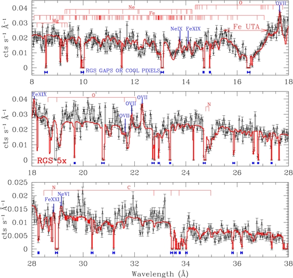
Figure 4. RGS spectrum of observation 5x together with the Model C fit (red) [8–38 Å]. The absorption lines are identified above; the corresponding transition and the main emission lines are marked in blue (top of the panel). The detector gaps or the cool pixels of RGS are marked in blue on the bottom of the panel (http://heasarc.gsfc.nasa.gov/docs/xmm/uhb/rgsmultipoint.html).
Download figure:
Standard image High-resolution image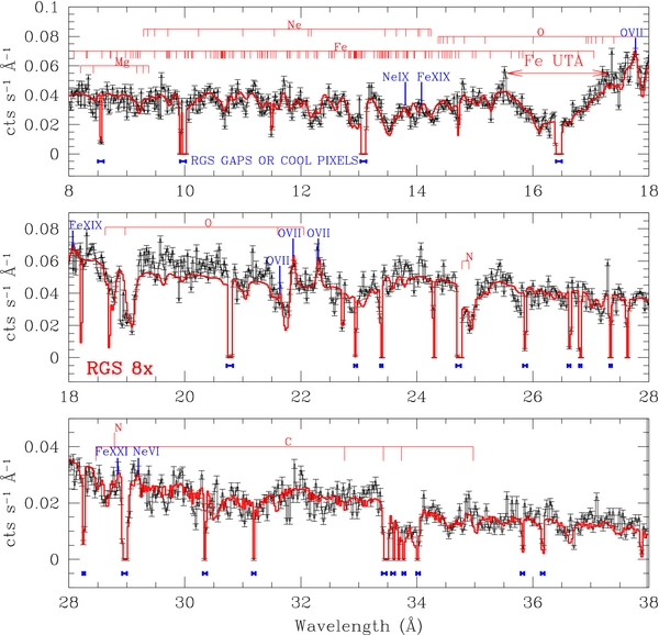
Figure 5. RGS spectrum of observation 8x together with the Model C fit (red) [8,38 Å]. The absorption lines are identified above; the corresponding transition and the main emission lines are marked in blue (top of the panel). The detector gaps or the cool pixels of RGS are marked in blue on the bottom of the panel (http://heasarc.gsfc.nasa.gov/docs/xmm/uhb/rgsmultipoint.html).
Download figure:
Standard image High-resolution image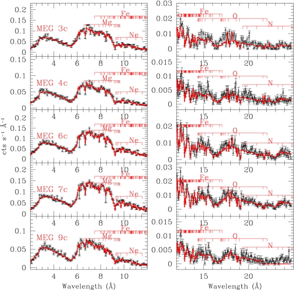
Figure 6. MEG spectra in [2–25 Å] range of each Chandra observation together with the Model C fit (red). The absorption lines are identified above with the corresponding transition (red).
Download figure:
Standard image High-resolution imageTable 9. Model C: All XMM-Newton and Chandra Observations
| Observation | Power Law | Blackbody | Phase HI | Phase MI | Phase LI | Statistics | |
|---|---|---|---|---|---|---|---|
| Γ | kT (keV) | logU | logU | logU | χred/dof | ||
| Norma | Normb | logNH | logNH | logNH | |||
| vout (km s−1) | vout (km s−1) | vout (km s−1) | |||||
| −1847 ± 350 | −605 ± 350 | −2426 ± 350 | |||||
| 1x | 1.82 ± 0.02 | 0.09 ± 0.02 | 1.76 ± 0.02 | 0.42 ± 0.02 | −1.07 ± 0.04 | 0.87/4504 | |
| 1.69 ± 0.02 |  |
22.33 ± 0.02 | 21.56 ± 0.02 | 21.13 ± 0.05 | |||
| −1847 ± 13 | −605 ± 27 | −2426 ± 5 | |||||
| 2x | 1.77 ± 0.02 | 1.77 ± 0.02 | 0.36 ± 0.02 | −0.73 ± 0.02 | 1.01/4558 | ||
| 1.33 ± 0.02 | 6.67 ± 0.05 |  |
21.46 ± 0.02 | 21.17 ± 0.03 | |||
| 3c |  |
 |
 |
 |
0.62/980 | ||
| 1.05 ± 0.02 | 4.14 ± 0.06 |  |
 |
 |
|||
| 4c |  |
2.05 ± 0.08 |  |
 |
0.68/980 | ||
| 0.66 ± 0.02 | 2.84 ± 0.04 | 22.22 ± 0.09 |  |
21.55 ± 0.06 | |||
| 5x | 1.62 ± 0.02 |  |
0.27 ± 0.03 | −1.13 ± 0.02 | 0.87/4504 | ||
 |
4.25 ± 0.06 | 22.49 ± 0.12 | 21.59 ± 0.02 |  |
|||
| 6c | 1.58 ± 0.02 | 2.24 ± 0.03 |  |
−0.54 ± 0.17 | 1.08/980 | ||
| 1.38 ± 0.03 | 5.65 ± 0.04 |  |
 |
 |
|||
| 7c | 1.69 ± 0.02 |  |
 |
 |
0.95/980 | ||
 |
6.13 ± 0.05 | 22.40 ± 0.05 |  |
 |
|||
| 8x | 1.75 ± 0.02 | 2.03 ± 0.02 | 0.45 ± 0.02 | −0.81 ± 0.04 | 0.95/4630 | ||
| 1.41 ± 0.02 | 5.33 ± 0.02 | 22.52 ± 0.02 | 21.47 ± 0.02 | 21.31 ± 0.02 | |||
| 9c |  |
 |
0.17 ± 0.15 |  |
0.74/980 | ||
 |
2.94 ± 0.05 |  |
21.57 ± 0.06 |  |
|||
Notes.
a In 10−2 photons keV−1 cm−2 s−1 in at 1 keV.
b In 10−4  .
.
Download table as: ASCIITypeset image
We further included in our models the fourth absorbing component (present only in the hard energy band), leaving free to vary independently among the observations the ionization parameter and column density, but constraining the outflow and turbulent velocities to a single best-fit value in all observations. Our results are summarized in Tables 9 and 10.
Table 10. Phase VH Applied in the Hard Band Spectra [3–10 keV], EPIC-PN of XMM-Newton, and HEG [3–7.7 keV] of Chandra
| Obs | VH.log U | VH.log NH | Statistics |
|---|---|---|---|
| χred/dof | |||
| 1x | 3.87 |
23.22 ± 0.02 | 0.65/1067 |
| 2x | 3.88 |
23.22 ± 0.02 | 0.81/1116 |
| 3c | 3.99±...a | 23.26 |
0.76/103 |
| 4c | 3.91 |
23.22 ± 0.06 | 1.25/103 |
| 5x | 3.88 ± 0.42 | 23.23 ± 0.02 | 0.78/1062 |
| 6c | 4.14 |
23.27 |
1.33/103 |
| 7c | 3.51 |
23.18 |
1.01/103 |
| 8x | 3.75 ± 1.08 | 23.22 ± 0.02 | 0.7/1188 |
| 9c | 3.49 |
23.28 |
0.82/103 |
Note. The outflow velocity is given by vout = −2650 ± 350 km s−1. a ... means indeterminate.
Download table as: ASCIITypeset image
Finally, given that the outflow velocities of components HI and LI are similar, we tried a model with these parameters linked to a single value for both components. The warm absorber best-fit parameters did not change significantly as with the Model C, Section 3.2. The velocity found for those two phases (phase HI and LI) is vout = −1905 ± 350 km s−1.
3.4. Fitting the Two Absorption Features in the Hard X-Ray Band of XMM-Newton and Chandra
We included in our models a fourth WA component with a very high ionization level to fit the two absorption lines detected in the hard band (these lines were initially identified with transitions by Fe xxv and Fe xxvi and fitted with Gaussians over the EPIC-PN data). This fourth absorber was modeled only on the EPIC-PN data of XMM-Newton from 3 to 10 keV and the HEG spectra of Chandra in the 3–7.7 keV hard X-ray band. An F-test gives us a confidence level larger than 99.99% for the existence of this absorber (hereafter VH) in all XMM-Newton observations. We found log U ∼ 3.8 and log NH ∼ 23.2 (see Table 10). Figure 7 shows the spectra and best fit over the EPIC-PN data.
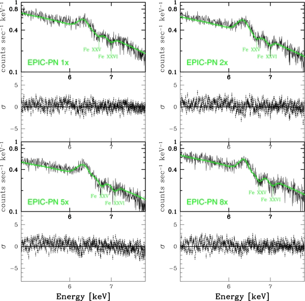
Figure 7. EPIC-PN spectra in the [5–8 keV] range of each XMM-Newton observation together with the power law function absorbed by phase VH fit (in green).
Download figure:
Standard image High-resolution imageIt is important to clarify that the hard X-rays were fitted separately from the soft X-ray band. However, to fix the power law in the soft energy band, we took into account the hard band in the fit, with the aim to have the best-fit value connected with the soft energy band. We also note that the soft absorbers have no effect on the hard energy band.
First, we fitted simultaneously three spectra of each XMM-Newton observation, RGS 1 & RGS 2 [8–38 Å: 0.33–1.55 keV] and EPIC-PN spectra in the energy range of 0.3–10 keV; the EPIC-PN spectra were included with the aim to obtain the best parameter of the power law. Then, we fitted the Fe–Kα emission line in 6.38 keV and two absorption lines of Fe xxv and xxvi in 6.7 and 6.96 keV, respectively. In this model (Model C), we included 10 emission lines in the soft energy band. Then model C was applied successfully in the five MEG [2–25 Å: 0.5–6.2 keV] and HEG spectra [1.6–15 Å: 0.8–7.7 keV], both Chandra high-resolution detectors. Finally, we cut the spectra of EPIC-PN from 3 to 10 keV and HEG spectra from 3 to 7.7 keV to obtain the fourth and highest ionized absorber, VH.
4. SUMMARY OF RESULTS AND COMPARISON WITH PREVIOUS WORKS
In order to study in detail the variability of the WA in NGC 3516, we have re-analyzed nine different individual observations from XMM-Newton and Chandra satellites. Our results show that the best-fit model for all spectra consists of a variable continuum emission absorbed by three partially ionized absorbers (WA) accounting for the soft band and a fourth highly ionized WA detected only in the hard band. Tables 9 and 10 summarize the values of the parameters of this model (Model C) for each observation. As can be observed in these tables, there are significant variations in some parameters of the model among the observations. In the following, we discuss the general properties of these absorbers and defer the time-resolved analysis for Section 4.1.
The different ionization components produce different absorption features. If we analyze them, we found that in the soft band, the highest ionized phase HI produces absorption by several Fe L-shell transitions with charge state xviii–xxii in the 10–16 Å range; absorption features by Si xiii–Si xiv (between 5–7 Å); Ne x absorption lines at 9.29, 9.36, 9.48, and 10.24 Å; and the O viii transition at 18.97 Å. Phase HI electron temperature is THI, e = 4.5 × 10⁵ K and the outflow velocity is vout, HI = −1847 ± 350 km s−1. Phase MI imprints absorption features due to O vii (at 16.96, 17.01, 17.09, 17.2, 17.4, 17.77, 18.62, and 21.6 Å), O viii (at 14.63, 14.45, 14.41, 14.82, 18.97 Å), and the most energetic portion of the Fe M-shell UTA (between 15 and 17 Å). The electron temperature associated with phase MI is given by TMI, e = 9.8 × 10⁴ K, while the outflow velocity is vout, MI = −605 ± 350 km s−1. Phase LI produces absorption lines by O vii at ∼16.9–18.6 Å and the low energy part of the M-shell Fe UTA (16.5–18 Å). This phase also produces absorption lines by Ne v–Ne vi between 12–14 Å. It has an electron temperature TLI, e = 3.0 × 10⁴ K and an outflow velocity vout, LI = −2426 ± 350 km s−1. Figure 8 shows the absorption features produced by each of the three absorbing phases (HI, MI, and LI).
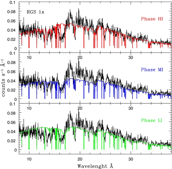
Figure 8. RGS spectrum of observation 1x (black) from 8 to 38 Å. Phase HI (top) is drawn in red; as can be observed, it reproduces absorption lines mainly in the lowest wavelengths of the spectrum. Phase MI (middle), in blue, reproduces the Fe M-shell UTA array and some absorption lines due to O vii and O viii transitions. Finally, phase LI (bottom), drawn in green, generates a fraction of the Fe-UTA and also the main absorption features around 18 Å.
Download figure:
Standard image High-resolution imageOn other hand, the fourth hard absorption phase VH produces the Fe K complex in the hard band. Its electronic temperature and outflow velocity are TVH = 7.0 × 10⁵ K and vout, VH = −2649 km s−1, respectively (see Table 9).
Given that several works have analyzed the 2006 X-ray spectra of this source, a comparison among different results is mandatory. In Table 11, we present the different parameters found in the different analyses. We note that the definition of the ionization parameter used by Turner et al. (2008) and Mehdipour et al. (2010) is different than the one presented here. These authors used the ionization parameter ξ,7 while our analysis was done with the parameter U (see footnote 6). Also, the SED is different in the different analyses. Therefore, a direct comparison of the ionization parameter is not possible. However, all works are in agreement in the sense that all require three different ionized absorbers, each imprinting absorption by similar charge states in the soft X-ray energy band. The fourth highly ionized absorber (found in the hard energy band) reported by Turner et al. (2008) as Zone 4 clearly corresponds with phase VH in this work.
Table 11. Comparison between the Warm Absorbers Found in Turner et al. (2008), Mehdipour et al. (2010), and This Work
| Model | WA 1 | WA 2 | WA 3 | WA 4 |
|---|---|---|---|---|
| Turner | Zone 1 | Zone 2 | Zone 3 | Zone 4 |
| logξ ∼ −0.05 | logξ ∼ 3 | logξ ∼ 2.5 | logξ ∼ 4.3 | |
| NH ∼ 6 × 1021 cm−2 | NH ∼1022 cm−2 | NH ∼1023 cm−2 | NH ∼1023 cm−2 | |
| vout = −200 km s−1 | vout = −1100 km s−1 | vout = −1100 km s−1 | vout = −1000 km s−1 | |
| Mehdipour | Phase A | Phase B | Phase C | |
| logξ = [0.87–0.97 ± 0.02] | logξ = [2.39–2.43 ± 0.05] | logξ = [2.99–3.07 ± 0.05] | ||
| NH = [0.33–0.43 ± 0.02] × 1022 cm−2 | NH = [1.7–3.2 ± 0.04] × 1022 cm−2 | NH = [1.2–1.7 ± 0.02] × 1022 cm−2 | ||
| vout = −100 to −200 ± 40 km s−1 | vout = −1500 to −1600 ± 100 km s−1 | vout = −800 to −1000 ± 300 km s−1 | ||
| Huerta | Phase LI | Phase MI | Phase HI | Phase VH |
| logU = −1.07 to −0.54 ± 0.17 | logU = [0.16–0.65] ± 0.04 | logU = [1.76–2.45] ± 0.05 | logU = [3.49–4.14] ± 0.06 | |
| NH = [0.13–0.34 ± 0.01] × 1022 cm−2 | NH = [0.25–0.40 ± 0.01] × 1022 cm−2 | NH = [1.66–3.31 ± 0.01] × 1022 cm−2 | NH = [1.51–1.90 ± 0.01] × 1023 cm−2 | |
| vout = −2426 ± 350 km s−1 | −605 ± 350 km s−1 | −1847 ± 350 km s−1 | −2650 ± 350 km s−1 | |
Notes. Ionization parameter ξ ≡ L/nr2, where L is 1–1000 Rydbergh luminosity, n the gas density, and r the absorber-source distance. Ionization parameter U ≡ (Q/4πR2nHc).
Download table as: ASCIITypeset image
Table 12. Covering Factor Values
| Obs. | 1x | 2x | 3c | 4c | 5x | 6c | 7c | 8x | 9c |
|---|---|---|---|---|---|---|---|---|---|
| Covering Factor % | 96% | 89% | 84% | 100% | 100% | 93% | 88% | 99% | 93% |
Note. The percentage of the covering factor presents a typical error of 5%.
Download table as: ASCIITypeset image
In general, the column densities are also in agreement among the different works. The column density NH of phase LI is similar to that reported by Turner et al. (2008) and Mehdipour et al. (2010). The values of NH for components HI and VH correspond to those by Turner et al. (2008) for Zone 3 and Zone 4, respectively. We note, however, that there is a significant difference in the column density of the mid-ionized absorber MI with respect to Zone 2 (Turner et al. 2008) and Phase B (Mehdipour et al. 2010). This change can be explained by the fact that we assumed full coverage for all absorbers in our analysis (but see Section 4.2.2).
The most intriguing difference in this work with respect to previous analyses is present in the different outflow velocities of the absorbers: phases LI, HI, and VH present outflow velocities significantly larger than previously found, while, phase MI presents a smaller outflow velocity than the components of middle ionization of these other works. It is worth mentioning that in Turner et al. (2005) the velocity of their Zone 1 was fixed to an outflow velocity of −200 km s−1, but in Turner et al. (2008), a value vout ∼ −1000 km s−1 is reported for this same component. Furthermore, Turner et al. (2008) based the outflow velocities on only 11 absorption lines (see their Table 1). Overall, the differences in velocity are likely produced because the different absorption lines are present with a range of velocities that are not fully resolved in the data.
This is further evidenced by Holczer & Behar (2012), who made a detailed analysis of the kinematic components in the high-resolution spectra of Chandra. They found evidence of four kinematic components with different outflow velocities. According to these authors, the slower components (with vout = −350 ± 100 km s−1 and vout = −1500 ± 150 km s−1) present a broad range of ionization, while the two faster components (vout = −2600 ± 200 km s−1 and vout = −4000 ± 400 km s−1) are more highly ionized. Phases MI, HI, and VH of the model proposed in this work are consistent with the results by Holczer & Behar (2012). The higher outflow velocity of component LI is discussed below in Section 5.2.
4.1. Time Variability
In this section, we perform a time-resolved analysis of the ionized absorber in NGC 3516. In particular, we identify the parameters that show significant variations among the observations and explore a possible correlation with the changes in flux.
4.1.1. Ionization Parameter U
Phase HI. The most significant change in ionization parameter is given at a 4σ level between observation 8x and the others. This parameter, along the nine observations, is plotted in Figure 9 (top plot). We also plot a scaled version of the flux values. This scaled version of the light curve represents the expected changes of U if the gas were instantly in photoionization equilibrium with the ionizing source (for gas in photoionization equilibrium, changes in flux must be followed by changes by the same factor in U). Clearly, this is not observed in Figure 9, indicating that there is no clear response of this component to the flux variations.
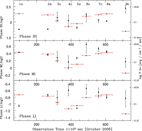
Figure 9. In all panels is plotted the light curve of the X-ray [8–25 Å] range of NGC 3516 (red); the flux energy Fhν was scaled in order to compare it with the logU parameter of each ionized phase. The logU variation in time is plotted for phases HI (top panel), MI (medium plot), and LI (bottom plot).
Download figure:
Standard image High-resolution imagePhase MI. This component presents strong significant changes between observations 1x and 5x at 7σ and between observations 5x to 8x at 8σ. Interestingly, these changes are correlated with the flux variations. Among observations 1x, 2x, 3c, and 4c, the ionization degree of the phase MI changes by nearly the same factor as the X-ray flux. This indicates that this component is responding to the continuum changes close to photoionization equilibrium.
Phase LI. The most important variations in U are found between observations 1x and 4c and between observations 2x and 5x, both at 4σ. For this phase, there is a reaction to the larger changes in flux in longer timescales, as observed in Figure 9 (bottom). From observations 2x and 4c the gas presents a delay in recombining as expected in photoionization equilibrium (PhE). Yet, at the time of observation 5x, the gas seems to have found equilibrium again. As the flux increases from observations 5x to 6c the gas re-ionizes to reach an ionization state consistent again with PhE. Overall, this component also seems to respond, albeit with larger delays and in a more complex way to the changes in the continuum.
Finally, we note that the highest ionization component VH (detected only in the hard X-ray band) does not present significant changes in the ionization parameter. This behavior is expected because the ionization potential of Fe xxv is 8.8 keV and that of Fe xxvi is 9.3 keV, and the hard X-rays always vary much less compared to the soft X-ray band. Therefore, it is possible that at these relevant energies, the continuum did not vary much. We conclude that the lack of variability cannot be used as a limit on density for this component.
4.1.2. Equivalent H Column Density
There are mild variations (by a factor of ≲2.5) in the H equivalent column density along the nine observations, for the three phases detected in the soft X-ray band. The variations are not anti-correlated with the energy flux, as it would be expected in a scenario where the WA consists of material crossing our line of sight, and this material was responsible for producing the flux variation observed in the light curve. Figure 10 shows the changes in this parameter of each ionized phase (phases HI, MI, and LI).
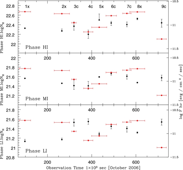
Figure 10. logNH variation in time is plotted for phases HI (top), MI (medium plot), and LI (bottom). The flux energy Fhν (in red) was scaled in order to compare it with the logNH parameter of each ionized phase.
Download figure:
Standard image High-resolution imageIn order to study how significant the changes are in column density, we performed a test, fitting all data sets with a single value of NH. The best-fit value for this parameter is similar to the values obtained when modeling individual observations, as expected. However, it is noteworthy that the other parameters are fully consistent with those obtained in Model C. In particular, the values for the ionization parameter are the same, within errors, as those found if NH is free to vary in each observation. This implies that the variations found in U are not produced or correlated by possible variations in the column density.
4.2. Variations in Spectral Features in the Spectra of NGC 3516
Given that the models predict variations in the ionization degree of two ionization phases (MI and LI), we have studied in detail the spectra of the source to identify clear signatures of such variations.
4.2.1. The Iron M-shell Unresolved Transition Array
This Fe M-shell UTA (Unresolved Transition Array) is extremely useful to look for opacity changes in the absorber phases (as shown by Krongold et al. 2005b). To look for these changes, we performed a comparison between spectra 1x and 5x in the 15–18 Å range. Both spectra were normalized using a simple power law to the local continuum. The residuals were overplotted to search for possible differences. The results are shown in Figure 11. An evident variation in the position of the Fe UTA can be observed between spectra 1x and 5x (upper panels in Figure 11).
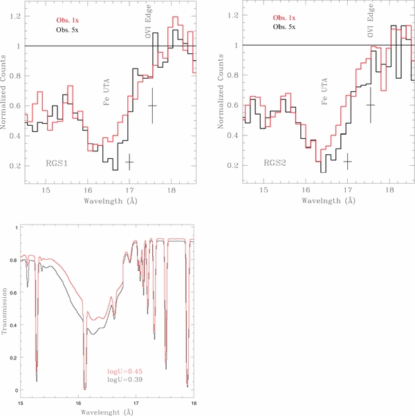
Figure 11. Fe M-shell UTA comparison between 1x and 5x spectra of RGS from XMM-Newton. For RGS 1 (left top panel) and for RGS 2 (right top panel) [14.5–18.5 Å]. In the bottom panel, the opacity variation produced by a change in the ionizing flux by a factor of two in photoionization equilibrium (modeled with the PHASE code; Krongold et al. 2003) is plotted.
Download figure:
Standard image High-resolution imageIn the bottom panel of Figure 11, we present the expected opacity changes in this spectral region in response to a variation by a factor of ∼ two in the ionizing flux. This change is similar to the flux variation between observations 1x and 5x, so it closely matches a scenario where the gas is in photoionization equilibrium. It is clear the observed variations are consistent with those expected in photoionization equilibrium for components MI and LI, which produce the UTA.
Figure 12 compares the Fe M-shell UTA between different Chandra spectra. This plot shows a similar variability trend (although less significant) between observations 4c and 6c, again pointing to gas close to photoionization equilibrium. Furthermore, no spectral variations are found between observations 6c and 7c, where the flux remains constant.

Figure 12. Fe M-shell UTA comparison between Chandra data from 15.5 to 18.5 Å range. Left: observations 4c and 6c. Right: observations 6c and 7c.
Download figure:
Standard image High-resolution image4.2.2. Testing Possible Changes in Covering Factor
The observed changes in column density (although not very drastic) could be produced by real changes in the total column density toward the source or by possible variations in the covering factor of partial covering absorbers. To further investigate this, and to explore if the changes in flux might be connected with changes in covering factor (as suggested by Turner et al. 2008), we have also looked at the two extreme XMM-Newton flux states (1x and 5x). We used two intense oxygen absorption lines, O viii-Kα and O vii-Kβ, to track these possible changes. As seen in Figure 8, these two lines track absorption by the three components found in the soft X-ray band. Given that these lines are saturated, their maximum depth should depend mainly on the fraction of the source covered by the absorber (i.e., the residual observed emission should give us directly the part of the source not covered). Therefore, changes in covering factor should produce variations in the depth of these lines. This is clearly shown in Figure 13 (upper left panel) where we present a model assuming a change in the covering factor from 40% to 70% (as reported in Turner et al. 2008). In Figure 13 (upper right and bottom panels), we present the normalized data for spectra 1x, 5x, 7c, and 9c. It is clear that the absorption lines do not change significantly between these states—the variations are within the error bars. Any possible variations do not follow the expected direction for a change in covering factor responsible for the flux changes. Rather, the data hint at a change where the absorption lines become deeper during the high states, as expected if the gas is responding to the changes in the continuum. The same comparison was performed among the Chandra data with similar results.

Figure 13. O vii–Kβ and O viii–Kα absorption lines [18–20 Å], the first panel (top) is the model assuming that the covering factor is changing. The second (bottom left) and third (bottom right) panels contain the O vii–Kβ and O viii–Kα absorption lines for observations 1x and 5x with the RGS1 and RGS2 from XMM, respectively.
Download figure:
Standard image High-resolution imageThe most striking result is obtained when comparing the Ne ix absorption feature between Chandra observations. As can be observed in Figure 14, there is a significant change in the depth of Ne ix transition, between observations 7c and 9c. This change can be easily understood as the response in the ionization state of the gas to the impinging flux. Furthermore, the change is exactly opposite to the one expected if the changes in flux were produced by changes in the covering factor.

Figure 14. Ne ix absorption line compared between Chandra observations 7c and 9c in the [13, 14 Å] range.
Download figure:
Standard image High-resolution imageTherefore, the high-resolution spectra do not support a scenario where the covering factor of the absorber is changing. This result is consistent with those of Mehdipour et al. (2010), who reached the same conclusion using data models. Thus, both data and models suggest that the changes in flux are not due to changes in the covering factor of the ionized absorber as suggested by Turner et al. (2008). Rather, our analysis (using models and direct comparison of spectra) indicates that the changes in spectral features are consistent with opacity changes following flux variations.
5. DISCUSSION
5.1. Location and Density of the Ionization Components
The time-variability analysis of the ionized absorber can lead us to constrain the number density of the gas and thus break the degeneracy between this quantity and the distance to the continuum source. As shown by Nicastro et al. (1999), the photoionization equilibrium time of a cloud of gas in response to variations in the ionized continuum is inversely proportional to the density of the cloud, according to the following formula:
where teq is the photoionization equilibrium time, Te is the electron temperature, and αrec(xi) is the radiative recombination rate coefficient (obtained from Shull & van Steenberg 1982 for the ions xi and xi + 1). We have used the response times detected in Section 4.1 to constrain the photoionization equilibrium timescale of the gas, and thus, the density of the gas.
5.1.1. Phase MI Location
The ionization state of this component follows closely the flux changes. Thus, the photoionization equilibrium timescale must be smaller than the typical elapsed time between observations. Using observations 4c to 5x, we find t1 = 15.12 ks (t1 is defined as the time between observations 4c to 5x), thus teq ≲ t1 = 15.12 ks.
Using the electronic temperature for this phase (Te = 9.8 × 10⁴ K) and the recombination rates for O vii and O viii, we find ne > 4.9 × 106 cm−3. From the measured value of U and the inferred luminosity of photons of the central engine (Q≅4.0 × 1053 photons s−1), this implies that the distance of component MI to the central source must be RMI < 3.4 × 1017 cm or RMI < 0.11 pc. Kraemer et al. (2002) estimated the dust sublimation radius of NGC 3516 as Rsub ≲ 2.7 × 1017 cm, assuming a dust sublimation temperature of 1500 K. Thus, this component is marginally consistent with the dust sublimation radius. However, we note that in the torus wind model of Krolik & Kriss (2001), the outflow must arise far beyond this radius, well into the "obscuring torus" (see Krongold et al. 2007 for a detailed discussion). Then, we consider more likely that this component arises from the accretion disk as suggested by Netzer et al. (2002).
5.1.2. Phase LI Location
According to the response observed in the ionization degree of the phase LI, two different timescales can be estimated. First, during the recombination phase from observations 2x and 4c this phase does not reach photoionization equilibrium with the impinging flux (see Figure 9). Therefore, teq > 125 ks, the time elapsed between these two observations. On the other hand, during the ionization episode between observations 5x and 6c, which lasted ∼50 ks, this absorbing component reached photoionization equilibrium with the source. We note that the different photoionization equilibrium timescales presented above are not incompatible with each other. Equilibration times are much longer during recombination phases than ionization ones. With these two constraints and the electron temperature of this component, Te, LI = 3.0 × 10⁴ K, we find a density 7.8 × 105 cm−3 ≲ ne, LI ≲ 1.9 × 106 cm−3. This in turn implies that the distance of this component to the central source should be between 1.8 × 1018 cm ≲ RLI ≲ 2.9 × 1018 cm. This component is likely arising from the dusty torus, as suggested by Krolik & Kriss (2001). However, we note that the flow might originate close to the region where we are observing it. Thus, a disk wind cannot be strictly ruled out.
5.1.3. Phase HI Location
The location of phase HI is more uncertain. The response timescale to the changes in the ionization flux should be greater than the duration of the low flux episode in the entire observation. From Figure 9, the low flux episode lasted ∼200 ks from observations 3c to 6c. Thus, the density for phase HI must be ne > 6.4 × 104 cm−3 (using a temperature of Te, HI = 4.5 × 10⁵ K and Fe xviii and Fe xix charge states). Therefore, the minimum distance to the central source for phase HI is RHI ∼ 4.0 × 1017 cm, which is around ∼0.13 pc. The location of this component is consistent with a flow arising in the dusty torus or a flow arising from the accretion disk observed further out.
As explained in Section 4.1.1, the lack of variation in component VH cannot be used to obtain a reliable constraint on distance, given that at higher energies the flux variations are much smaller.
5.2. Does the Absorber Form a Multi-phase Medium?
It has been suggested by several studies (e.g., Krongold et al. 2003, 2005a, 2005b; Cardaci et al. 2009) that the structure of ionized absorbers could be that of a multi-phase medium in pressure balance. A multi-phase medium requires absorbers with similar outflow velocities to avoid drag forces from destroying one of the components. Clearly, component MI cannot be part of the same flow as components LI and HI, as these components are located farther out from the central source and they have a much faster outflow velocity. However, components LI and HI have a similar outflow velocity and they may be located at a similar distance from the central source. Then, it is possible that these components indeed form a multi-phase medium.
In order to further study this possibility, the thermal equilibrium (S curve) obtained for the SED in this analysis is plotted in Figure 15. This curve presents the points where the gas temperature (log T) and pressure lie in thermal equilibrium. The gas pressure is inversely proportional to the quantity log(U/T), which can be directly derived in our analysis. Thus, two components can be part of a multi-phase flow if they have different temperatures but similar log(U/T) values. Assuming solar metallicities (Z☉) the S curve for NGC 3516 (Figure 15) is not multi-valued. Thus, it is not possible that these two components exist in pressure equilibrium.
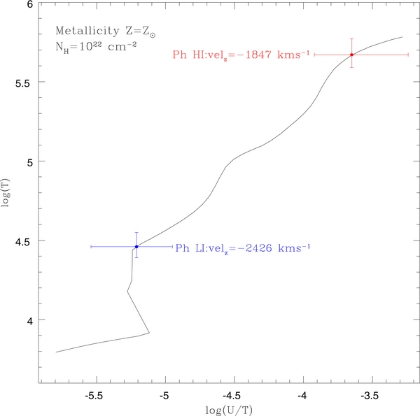
Figure 15. Thermal stability curve S of NGC 3516 SED supposing log NH = 1022 cm−2 and a solar metallicity Z☉. Over-plotted there are the ionized absorbers HI and LI.
Download figure:
Standard image High-resolution imageHowever, the shape of the S-curve results is very sensitive to external heating and cooling sources. Additional cooling can be produced by material with metallicities higher than the solar one. In fact, in AGNs, supra-solar metallicities are expected (e.g., Mihalszki & Ferland 1983 and Fields et al. 2007). A higher amount of cooling material creates a more vertical S-curve and together a possible "multi-phase" system. With the goal to explore this possibility, we present a model with five times solar metallicity (5 Z☉). Figure 16 shows that if the metallicity of the WA is higher than solar, then components LI and HI could coexist in pressure equilibrium given that the pressure of both absorbers are in the same order of magnitude. As seen in the plot for a metallicity of 5 Z☉, the difference between the gas pressure of these components is not significant.

Figure 16. Thermal stability S curve of NGC 3516 SED supposing log NH = 1022 cm−2 and supra-solar metallicity 5 Z☉. Over-plotted there are the ionized absorbers HI and LI.
Download figure:
Standard image High-resolution image
5.3. Intrinsic Variability versus Obscuration Scenarios for the Flux Changes in NGC 3516
Two possible scenarios have been suggested to explain the observed variability in the X-ray emission of NGC 3516. The first one suggests intrinsic variations of the central source (Mehdipour et al. 2010). In the second scenario, explored by Turner et al. (2008) and Markowitz et al. (2008), they proposed that the variations are due to obscuration of the central source produced by nearby blobs of material, either ionized or neutral. In particular, Turner et al. (2008) suggest that an absorbing component of ionized material (their "heavy absorber") presents a change in the covering factor, which is responsible for the observed flux variations. Such component would produce absorption by ions of O viii and O vii (Turner et al. 2008). However, we could not find evidence of covering factor variations in the O vii–Kβ and O viii–Kα lines (Figure 13).
To further explore this possibility, we fit the spectra using a partial covering absorber. We note that partial covering is not required by the data, as a fit including it does not improve over a fit with fully covering absorbers (in agreement with Mehdipour et al. 2010). Nevertheless, based on Model C, a partial covering was tested in all the possible combinations, including this factor, in one, two, and three ionizing components that imprint spectral features in the soft X-ray band.
The best solution found included partial covering in phase HI. However, the value of the covering factor is almost unity in all observations (see Table 12), and does not anti-correlate with the flux. An F-test indicates that varying the covering factor is not needed (confidence of 57% if we compare the model that does not include the covering factor and this model). Thus our results do not support a scenario in which the covering factor of the warm absorbers is responsible for the flux variations. If these variation are indeed produced by obscuring material, this material should be located closer in than the warm absorbing components, as components LI and MI are responding to the observed flux variations.
6. CONCLUSIONS
We summarize our results as follows.
- 1.We modeled the nine X-ray 2006 data of XMM-Newton and Chandra. The best statistical model consists of a complex and variable continuum emission component and also includes nine emission lines of different ionized species in the soft X-ray band. An additional emission line is required in the hard X-ray band, where the Fe–Kα emission line is present. The continuum emission is absorbed by four different ionized phases (warm absorbers): three of them produce features in the soft X-ray band and the fourth, with the highest ionization degree, only generates the Fe–Kα absorber complex detected in the 6.7–7 keV range.
- 2.The ionization state of the two components with the lowest ionization degree (phases MI and LI) is responding to the changes in the ionizing continuum. The other two absorbing components (phases VH and HI) do not seem to react to the ionizing continuum variations.
- 3.The observed variations in the Fe M-shell UTA (produced by phases MI and LI) between observations 1x and 5x were found to be similar to what is expected for ionized material close to photoionization equilibrium.
- 4.The response timescale of the phases MI and LI allow us to constrain their location: for phase MI the location is RMI < 2.7 × 1017 cm. For component LI, the location must be within the range 1.8 × 1018 cm ≲ RMI ≲ 2.9 × 1018 cm. For component HI, a lower limit to the location was derived: RHI ≳ 4.0 × 1017 cm. The lack of variations in component VH cannot be used to find a reliable constraint on its location (see Section 4.1.1).
- 5.There is no evidence of a depth change in the main absorber transitions (O vii-Kβ, O viii–Kα and Ne ix), as expected in a scenario where the covering factor is varying in the time.
- 6.Finally, if solar metallicity is assumed (Z☉), the absorbing components cannot be in pressure equilibrium. However, with higher metallicity values (5 Z☉) the S-curve becomes more vertical and then it becomes possible that the absorbers HI and LI form a multi-phase medium.
We thank the referee for thoughtful and constructive comments that helped to improve the paper. We also thank Doron Chelouche, Maria Santos-Lleo, and Ehur Behar for their invaluable help and constructive comments. This research is based on observations obtained with XMM-Newton, an ESA science mission with instruments and contributions directly funded by ESA Member States, and the Chandra Space Telescope of NASA.
Footnotes
- 6
Ionization parameter: U = Q/(4πR2nHc), where Q is the rate of 0.013–100 keV photons produced in the source, R the distance between the black hole and the accretion disk system to WA location, nH the hydrogen number density, and c the light speed.
- 7
Ionization parameter ξ: ξ ≡ L/nr2, where L is 1–1000 Rydbergh luminosity, n the gas density, and r the absorber–source distance.