


ABSTRACT
Recent in-situ determinations of the temporal evolution of the charge state distribution in the fast and slow solar wind have shown a general decrease in the degree of ionization of all the elements in the solar wind along solar cycles 23 and 24. Such a decrease has been interpreted as a cooling of the solar corona which occurred during the decline and minimum phase of solar cycle 23 from 2000 to 2010. In the present work, we investigate whether spectroscopic determinations of the temperature of the quiescent streamers show signatures of coronal plasma cooling during cycles 23 and 24. We measure the coronal electron density and thermal structure at the base of 60 quiescent streamers observed from 1996 to 2013 by SOHO/SUMER and Hinode/EIS and find that both quantities do now show any significant dependence on the solar cycle. We argue that if the slow solar wind is accelerated from the solar photosphere or chromosphere, the measured decrease in the in-situ wind charge state distribution might be due to an increased efficiency in the wind acceleration mechanism at low altitudes. If the slow wind originates from the corona, a combination of density and wind acceleration changes may be responsible for the in-situ results.
Export citation and abstract BibTeX RIS
1. INTRODUCTION—THE SUN IN TIME
Since the discovery that the temperature of the solar coronal plasma exceeds one million degree Kelvin, and that the solar corona emits a continuous, roughly bimodal stream of particles called the solar wind, several decades of continuous studies have been devoted to understanding both how the corona is heated and the solar wind is accelerated. Such an understanding has become increasingly important for our society, as the Sun ultimately provides the energy that drives the Earth's climate, controls the interplanetary medium in which the Earth is immersed, and is the origin of space weather events that can significantly affect space- and ground-based human assets. However, despite all the efforts, we have not yet reached a satisfactory understanding of the problems of coronal heating and solar wind origin.
Recently, the success and longevity of the space missions devoted to observing the Sun in the X-ray, EUV, and UV wavelength ranges, as well as to measuring the in-situ properties of the solar wind, allow us to approach the problems of coronal heating and wind origin from a new point of view: their long-term evolution. In fact, the availability of almost 17 yr of continuous observations of the solar corona with high-resolution spectrometers now allows us to carry out diagnostic studies of coronal plasmas encompassing the entirety of solar cycle 23 and the first half of solar cycle 24. At the same time, systematic measurements of charge state composition, wind properties, and element abundances have been available since the early 1990s. These data allow us to investigate whether there are any patterns or cycle-related changes in the properties of both the solar wind and the inner solar corona and to see whether they are related to each other. Such studies are particularly timely, since the current solar cycle 24 has been unexpectedly anomalous, showing a smaller number of sunspots and the lowest level of activity since the beginning of the space age in the 1950s (Smith & Balogh 2008; McComas et al. 2008; de Toma et al. 2010; Gibson et al. 2011). However, it has been shown that rather than being exceptionally weak, solar cycle 24 is actually much more in line with the cycles in the past 250 yr and that the last 4–5 solar cycles were unusually strong (McCracken et al. 2013). Thus, for the first time since the beginning of the Space Age, the effects of the solar cycle on the heating of the solar corona and the origin of the solar wind can be studied while the Sun is returning to its normal state after spending the last 4–5 solar cycles in an enhanced activity state.
1.1. The Solar Wind
Recent studies of the WIND, Ulysses, and ACE decade-long measurements of the charge state composition of the solar wind by Kasper et al. (2012), von Steiger & Zurbuchen (2011), and Lepri et al. (2013), respectively, have provided a more detailed and quantitative assessment of the effect of the solar cycle on the in-situ properties of the wind plasma. By monitoring the plasma composition from the maximum of solar cycle 23 to the unusually weak minimum of solar cycle 23, those studies found that the charge state ratios of C and O, as well as the average charge states of Si and Fe, decreased significantly. Such a decrease led the authors to conclude that the solar corona cooled both in the polar and equatorial regions during the decline of solar cycle 23 and the subsequent minimum. This cooling was then followed by a rise in coronal temperatures at the beginning of cycle 24. Changes in the element abundances of wind plasmas relative to oxygen were found by Lepri et al. (2013), and a decline in the absolute abundance of heavy ions was also found by Kasper et al. (2012; He) and Lepri et al. (2013; C, O, Si and Fe).
For example, Figure 1 shows the coronal electron temperature inferred from the O7 +/O6 + as measured by ACE/SWICS from 1998 to 2011. We will refer to the temperature measured from in-situ charge state ratios as  . The number density of each ion involved in the ratio was obtained by integrating the solar wind ion flux for two hours, and the electron temperature was determined by comparing the daily average of the measured values with estimates of the charge state ratio calculated under the assumption of ionization equilibrium with CHIANTI V 7.1 (Landi et al. 2013). Data measured during interplanetary coronal mass ejections were excluded, while both types of solar wind were included. The left panel shows the distribution of daily temperatures as a function of time, and the right panel shows their monthly average. Figure 1 clearly shows a continuous, steady decline of the wind source region temperature regardless of wind type, followed by a rise at the beginning of the rise phase of cycle 24. Most importantly, Figure 1 shows that
  closely follows the phase of the solar cycle, indicated by the monthly sunspot number (full line in both panels, scaled to adjust to the temperature limits).

Figure 1. Coronal electron temperature  measured with daily averages of O7 +/O6 + charge state ratios from ACE/SWICS. Left: distribution of temperatures as a function of time. Right: monthly averages. The curves superimposed to the temperature measurements (white in the left panel, blue in the right panel) represent the monthly sunspot number, scaled to match the level of the temperature measurements.
Download figure:
Standard image High-resolution imageSchwadron et al. (2011) noted the same decrease in the  values and correlated it to lower particle fluxes occurring in the same time period. They interpreted this correlation as due to a cooling of the solar corona, through the Schwadron & McComas (2003) solar wind scaling law: assuming a fixed energy per particle input, the energy per particle lost from the corona through downward heating flux scales as
  , where Tm is the maximum coronal temperature at or below a scale height. They argue that a reduction in wind particle flux and Tm need to occur in order to maintain the same wind speed, and thus they conclude that the temperature of the solar corona needs to decrease.
Interestingly, Habbal et al. (2010) studied the average charge state of Fe, as distributed by the ACE/SWICS team, from 1998 to 2009, and found different results. They first noted that the average charge state of Fe did not change much in time, something also noted later by Lepri et al. (2013). Second, they showed that the in-situ Fe charge state distribution corresponding to the eclipses of 2006 March 29 and 2008 August 1 matched the ion fractions of the Fe ions observed in the inner corona, so that the former could be used as a proxy for the latter, and thus they could be used as a tool to measure the temperature of the solar corona. Third, using the in-situ Fe charge states they showed that the near constancy of the average Fe charge state indicated that the coronal temperature did not change over solar cycle 23, at temperatures around 1.1 × 10⁶ K. Similar results are obtained using ratios between the frozen-in charge states of carbon measured by ACE: even if such ratios can be very efficiently used to determine the temperature of the solar corona in the same way as the oxygen charge states, they showed only a very mild dependence on the solar cycle.
The apparent decrease of the coronal electron temperature in Figure 1 can be due to a variety of factors. However, the fact that Fe ions and carbon ions show little variation seems to suggest that the coronal temperature might not be the only factor that has influenced the O7 +/O6 + ratio. In fact, the charge state ratios measured by ACE are the end result of the evolution of the ionization status of the wind plasma from the wind source region to the freeze-in point. This evolution is largely dominated by the three wind parameters that rule the amount of ionizations and recombinations experienced by the wind plasma along its journey: the electron density and the electron temperature, which determine the local value of the ionization and recombination rates at any given location along the wind trajectory, and the wind velocity, which determines how much time the solar wind spends at such location (e.g., Landi et al. 2012a and references therein). Thus, changes in the O7 +/O6 + charge state ratios, such as those shown in Figure 1, can be due not only to temperature variations, but also to changes in the wind electron density and speed close to the Sun, or combinations of these three parameters. Such changes occur in the regions of the solar corona where both the carbon and oxygen charge state distributions freeze but do not affect carbon charge states as efficiently. Conversely, the moderate variations of the Fe charge state distribution over time indicate that the coronal regions where the Fe charge state distribution freezes in did not change appreciably during the entire solar cycle 23.
1.2. The Solar Corona in Time
In-situ measurements alone cannot easily answer the question of which of these three parameters (or which combination of them) is responsible for the measured changes in the wind charge states. Also, they provide different results when using different elements. Since the charge state composition of the solar wind is largely determined in the inner corona (e.g., Ko et al. 1996; Chen et al. 2003; Landi et al. 2012a and references therein), remote sensing observations can provide indications of long-term variations in some of these parameters. In particular, remote sensing instruments observing the inner corona (e.g., below 1.5 solar radii) can determine the physical properties of the regions where the lightest elements (e.g., C, O) freeze in.
It is common knowledge that the solar corona undergoes dramatic changes of activity during each solar cycle and from one cycle to the next, as the number, size, and energy of active regions are strongly dependent on the magnetic fields in the same sunspots that define the phase of the solar cycle itself (e.g., Peres et al. 2000). Also, long-term changes in the irradiances of EUV coronal emission lines were found to correlate with the solar cycle, especially when emitted by hot plasmas (Del Zanna & Andretta 2011). However, both the fast and slow solar wind come from other sources than active regions. While some fast streams of plasma have been observed to come from the sides of active regions (Brooks & Warren 2011; Slemzin et al. 2013 and references therein), the bulk of the fast solar wind is accelerated from polar and equatorial coronal holes, while the slow solar wind is accelerated from a still unknown region of quiescent streamers. Thus, to monitor cycle-dependent effects on the wind, it is necessary to study the long-term evolution of the properties of coronal holes and quiet streamers.
A few studies have measured the properties of selected portions of the solar corona as a function of time. For example, studying the time evolution of the intensities of several lines observed by Hinode/EIS at the disk center between 2006 and early 2011, Kamio & Mariska (2012) found that the intensities of hotter lines show significant temporal variations, while those of the cooler lines, formed around 0.8–1.1 MK, are much less variable. Similarly, Orlando et al. (2001) found that the temperature of the regions with low Yohkoh X-ray fluxes, interpreted as quiescent regions, was, on average, constant between solar maximum and minimum. Both studies point in the direction of a rather constant quiet coronal plasma sitting next to a more cycle-dependent and variable hotter component confined in magnetic field structures, which prevent these two plasmas from influencing each other.
A similar result was obtained using X-ray observations integrated over the entire Sun. For example, Argiroffi et al. (2008) studied Yohkoh and GOES observations in the 1991–1999 period, encompassing the maximum of solar cycle 22, the minimum between cycles 22 and 23, and the rise phase of cycle 23. They found that the emission measure (EM) of the entire Sun could be divided in two components, a flaring one and a quiescent one; the former showed a very strong dependence on the solar cycle with a marked decrease at solar minimum, and the latter, while decreasing toward solar minimum, showed far less variation with time. Peres et al. (2000) found that the average temperature of the Sun decreased as the solar cycle approached the minimum. By using X-rays, these studies were likely sampling the hotter component of the non-flaring plasmas, and thus their results correspond to those obtained by Kamio & Mariska for the lines from the hotter component of non-flaring plasmas.
Visible coronographic observations provide simultaneous 2D images of the entire solar corona and can be used to determine its electron temperature for long periods of time. Using the Fe x and Fe xiv visible lines, Guhathakurta et al. (1993) determined the temperature at all latitudes at the height of 1.15 Rsun from 1984 to 1993 (encompassing the maximum of cycle 22), finding that, outside the regions of larger activity, the coronal temperature showed little variation. A similar study was carried out by Altrock (2004), who used the same lines to measure the coronal temperature over a larger period of time (cycles 21 to 23), differentiating between polar regions with latitude ∣λ∣ > 80° and those at mid latitudes (30° < ∣λ∣ < 80°). While polar temperatures showed a marked dependence on the cycle, likely due to the alternating presence of coronal holes during minimum and quiet regions during maximum, at mid-latitudes, the temperature showed a far smaller temporal variability; while not constant, the variation is limited to a few tens of thousand K, corresponding to only a few percent.
At larger heights above the limb, UVCS and LASCO observations were used to build wind velocity and density estimates from 1996 May to 2008 August, during the rise phase of cycle 23 by Strachan et al. (2012). Measurements of wind velocity and density were provided at 2.3 Rsun, and it was found that at that height, the outflow velocity decreased at all latitudes, while the plasma density showed a large increase at low latitudes and a small increase in polar holes. At the same time, the plasma proton temperature increased at the poles and decreased at low latitudes.
Kamio & Mariska (2012) also showed that the electron density of the quiet Sun, measured using a Si x line intensity ratio, was constant within a factor less than two in the data they used in the 2006–2011 interval; since Si x absolute line intensities showed temporal variations, they attributed the latter changes to evolution in the plasma filling factor f, or in the depth of the line of sight at disk center.
The study of Orlando et al. (2001) was, however, based on data at the limit of the Yohkoh sensitivity because the instrumental temperature response functions were (1) less sensitive to quiet Sun temperatures and (2) less accurate, given that the atomic data available at the time of that study have been largely updated with more recent and accurate calculations (Landi et al. 2006, 2013). On the other hand, Kamio & Mariska (2012) used much more sensitive EIS spectral lines but confined their studies only to a 5 yr long time period, encompassing mostly the minimum phase of solar cycle 23. Also, they used disk center observations, where the line of sight encompasses the entire solar atmosphere from the chromosphere to the corona, so that their low-temperature line intensities may be affected by contribution of the upper transition region.
The goal of the present paper is to utilize high-resolution spectral observations of the quiescent solar corona to extend the work of Altrock (2004) and determine whether the plasma electron temperature has changed during the entire solar cycle 23. The novelty of the present work is twofold: first, it includes solar cycle 23 and the anomalous minimum between cycles 23 and 24, as well as the rise of the very weak cycle 24. Second, rather than relying on only two coronal visible lines or indirect proxies, it makes use of the full temperature diagnostic potential of the high-resolution spectrometers on board SOHO and Hinode.
We focus on quiescent streamers, thought to host the source regions of the slow solar wind, and determine the temperature structure of some of them from 1996, when the SOHO EUV spectra of the Sun became available, to early 2013. We will use off-limb observations to minimize the contamination of the coronal spectra by colder plasmas. The choice of streamers has two advantages: first, they can be found in the Sun at all times during the solar cycle, while coronal holes, the source of the fast wind, are more difficult to observe during solar maximum; second, the thermal structure of several streamers has been found to be rather simple, often consisting of a single peak distribution centered around 1.5 MK (e.g., Feldman & Landi 2008 and references therein).
In Section 2, we introduce the methodology we use to measure the thermal structure of each streamer, while in Section 3, we describe the observations we used. Section 4 introduces the results, which will be discussed in Section 5.
2. DIAGNOSTIC METHOD
In the present work, we determine the thermal structure of off-disk quiescent streamers and measure plasma electron density using standard diagnostic techniques. The intensity of an optically thin emission line can be written as
where Ne is the electron density, V is the emitting volume along the line of sight, d is the distance between the emitting source and the observer, and G(T, Ne) is the Contribution Function of the emitting line defined as
where (Nj(X+m)/N(X+m)) is the relative population of the upper level j, (N(X+m)/N(X)) is the relative abundance of the ion X+m (the ion fraction), (N(X)/N(H)) is the abundance of the element X relative to hydrogen, (N(H)/Ne) is the hydrogen abundance relative to the electron density (≈0.83 for fully ionized plasmas), and A is the Einstein coefficient for spontaneous emission. To calculate the contribution function, we used the latest version of CHIANTI (7.1.3, Landi et al. 2013), the latest CHIANTI ionization equilibrium rates (chianti.ioneq file available in CHIANTI 7.1.3), and the coronal abundances of Feldman et al. (1992).
When the plasma is multithermal, Equation (1) can be rewritten by defining the differential emission measure (DEM), φ(T), as
The DEM indicates the amount of material in the plasma as a function of temperature. Several different methods to determine φ(T) from Equation (3) have been developed, and they are reviewed by Harrison & Thompson (1992) and Phillips et al. (2008). In this work, we use the Markov-Chain Monte Carlo (MCMC) technique developed by Kashyap & Drake (1998). The MCMC technique is based on a Bayesian statistical formalism that allows the determination of the most probable DEM curve that reproduces the observed line intensities. The heart of this technique relies on the application of the Bayes theorem to line intensities, stating that the probability P(X, I) of obtaining a set of observed line intensities I = (I1, I2, ..., In) from a DEM characterized by a set of parameters X = (X1, X2, ..., Xm) is given by
where P(I) is a normalization factor, P(X) is an a priori probability of the set of parameters X, and P(X, Ii) is the probability of obtaining the observed intensity Ii with the set of parameters X. Kashyap & Drake (1998) defined P(X, Ii) as

where  is the intensity of line i calculated with the DEM described by the set of parameters X, and σi is the uncertainty of the observed intensity Ii. In this method, the DEM is discretized in N temperature bins, each associated to an EM value EMi, so that X = (EM1, ..., EMN).
The set of parameters, X, that describes an initial arbitrary trial DEM is varied step by step; in each step, only one of the EMi values is varied. The new set of parameters, X', is accepted or rejected according to the Metropolis algorithm (Metropolis et al. 1953): a random number u is generated, such that 0 ⩽ u < 1, and a function A(X, X') is defined as
The new set of parameters is accepted if u < A(X, X') and rejected otherwise. In this way, a new set of parameters X' yielding a greater probability is always accepted (A(X, X') = 1), and a new set with a smaller probability has a finite chance of being accepted. This latter property helps in finding the best distribution of parameters X by moving the solution out of local maxima. When the system has found the best solution, the distribution of the EM values in each bin found in all steps is used to determine the confidence interval at each temperature, providing an estimate of the uncertainty of the DEM at all temperatures.
The MCMC technique discretizes the solution using temperature bins of finite size, so that it is possible to have multiple DEM peaks at very similar temperatures. The question is whether such peaks are real and describe two distinct plasmas, or whether they are an artifact of noise or other factors, such as a limited number of available spectral lines; also, it is important to understand whether isolated peaks indicate truly isothermal plasmas or not. Landi et al. (2012b) used synthetic line intensities calculated with ad-hoc, predetermined DEM curves to test the ability of the MCMC technique at (1) retrieving the peak temperature of isothermal plasmas; (2) discriminating between an isothermal plasma and a plasma with a narrow temperature distribution; and (3) resolving the presence of multiple, near-isothermal plasma structures. Landi et al. (2012b) found that the MCMC technique is unable to retrieve isothermal plasmas to better than Δlog T ≃ 0.05. More importantly, two near-isothermal components can be unambiguously resolved only if their temperature separation is Δlog T = 0.2 or larger. This result is in agreement with a study by Testa et al. (2012), who explored the reliability of DEM reconstructions based on synthetic EUV spectroscopic (EIS) and imaging (AIA) data from 3D MHD models. They find that also using spectroscopic data, which provide significantly better constraints than imaging data, thermal features on scales of Δlog T ≲ 0.2 cannot be trusted.
3. OBSERVATIONS
In order to sample the thermal properties of off-disk quiescent streamers in the whole 1996–2013 time range, we have used two instruments: SOHO/SUMER and Hinode/EIS. We did not use SOHO/UVCS as it observes too high in the atmosphere for the goals of the present work; we preferred SUMER over CDS because of the better spectral resolution of the former after the SOHO loss of attitude in June 1998. In fact, the present study relies on the use of lines from many different ions but the decreased post-1998 spectral resolution of CDS limits the number of available lines. On the contrary, SUMER spectral resolution survived the accident so that this instrument preserved its diagnostic capabilities intact. The downside of the use of SUMER is the relative dearth of observations in the 2001–2006 period, due to the fact that SUMER carried out observations only a few times a year in dedicated campaigns. For both instruments, we used data sets that maximized the number of ions available for analysis because a large number of ions formed at many different temperatures is required to reconstruct the DEM curve with accuracy and for an extended temperature range.
3.1. SUMER Observations
The SUMER instrument on board SOHO is a high spectral and spatial resolution normal incidence spectrometer described in detail by Wilhelm et al. (1995), Wilhelm et al. (1997), and Lemaire et al. (1997). SUMER can observe in the 500–1600 Å range with a spatial resolution of 1 arcsec and a ≃43 mÅ pixel spectral size; however, the instrumental configuration allows only ≃ 40 Å-wide spectral windows to be simultaneously imaged on the detector.
For the present work, we selected observations carried out using the REFSPEC observing program. REFSPEC spectra include the entire wavelength range of SUMER. The dates and main characteristics of the observations are reported in Table 1, along with the height of the selected spectrum and plasma electron density at that height (see Section 4.1). The REFSPEC sequence consists in one single pointing of the slit (sit'n'stare mode), so the slit size corresponds to the total field of view of the entire observation. In each spectrum, we averaged over several pixels in order to increase the signal-to-noise ratio; these pixels were selected as those closest to the solar limb. All SUMER observations were selected to be far from any active region or coronal hole structure.
Table 1. Details of the SUMER Observations
| Date | Time | FOV Center | Slit | Exp. Time (s) | Rsel | log Ne |
|---|---|---|---|---|---|---|
| 1996 Apr 23 | 02:02–07:16 | 4'' × 300'' | (−1100'', 0'') | 300 | 1.140 | 8.00 ± 0.15 |
| 1996 Jun 19 | 02:20–07:34 | 4'' × 300'' | (−980'', 150'') | 300 | 1.030 | 8.00 ± 0.25 |
| 1996 Jul 23 | 01:52–06:50 | 1'' × 300'' | (−980'', 0'') | 300 | 1.030 | 8.35 ± 0.30 |
| 1996 Oct 1 | 21:21–02:29 | 1'' × 300'' | (1020'', −100'') | 300 | 1.060 |  |
| 1996 Nov 21 | 21:16–06:06 | 1'' × 300'' | (0'', 1160'') | 300 | 1.030 ± 0.005 | 8.25 ± 0.30 |
| 1997 May 8 | 01:58–07:05 | 1'' × 300'' | (700'', 820'') | 300 | 1.040 ± 0.005 | 8.25 ± 0.15 |
| 1997 Jun 12 | 12:00–02:11 | 4'' × 300'' | (600'', 1020'') | 300 | 1.114 ± 0.006 | 7.70 ± 0.30 |
| 1997 Jul 28 | 13:01–05:32 | 1'' × 300'' | (650'', −900'') | 300 | 1.050 ± 0.010 | 7.90 ± 0.20 |
| 1998 Feb 11 | 01:30–06:36 | 4'' × 300'' | (1030'', −300'') | 300 | 1.065 ± 0.005 | 8.00 ± 0.25 |
| 1999 Feb 23 | 21:52–03:00 | 1'' × 300'' | (0'', −1168'') | 300 | 1.040 ± 0.005 | 8.00 ± 0.20 |
| 1999 Mar 19 | 01:55–07:08 | 1'' × 300'' | (−850'', 700'') | 300 | 1.040 ± 0.002 | 8.50 ± 0.30 |
| 1999 Apr 30 | 22:45–06:59 | 1'' × 300'' | (−1002'', −245'') | 265 | 1.058 ± 0.005 | 8.20 ± 0.30 |
| 2000 Jun 13/20 | seven days | 4'' × 300'' | (−600'', 941'') | 300 | 1.050 ± 0.01 | 8.20 ± 0.20 |
| 2001 Mar 25 | 00:54–08:53 | 4'' × 300'' | (954'', 525'') | 300 | 1.045 ± 0.010 | 8.15 ± 0.25 |
| 2002 May 26 | 11:01–17:21 | 0.3'' × 120'' | (940'', 530'') | 370 | 1.115 ± 0.005 | 8.30 ± 0.30 |
| 2004 Jun 7 | 23:29–05:48 | 1'' × 120'' | (890'', 420'') | 370 | 1.025 ± 0.005 | 8.25 ± 0.20 |
| 2005 Jun 5 | 16:04–23:01 | 1'' × 120'' | (−900'', 413'') | 200 | 1.100 ± 0.005 | 7.95 ± 0.30 |
Notes. The uncertainties in Rsel indicate the range of heights where the spectrum was averaged. Values without uncertainties were averaged from an area at the same distance from the Sun.
Download table as: ASCIITypeset image
Data reduction was carried out using the standard SUMER software available in SolarSoft, accounting for flat field, geometrical corrections, and intensity calibration; residual geometrical distortions were removed by the authors. Since the intensities were measured in regions close to the limb selecting bright transitions, the effects of instrument-scattered light are negligible.
3.2. EIS Observations
The EIS instrument on board Hinode is described in Culhane et al. (2007) and observes two wavelength ranges simultaneously: 170–212 Å and 246–292 Å. A variety of different observing sequences have been employed to obtain the data we used. Their main characteristics are listed in Table 2; in all cases, they included a large amount of ions so that the resulting DEM determination was as accurate as possible. Their fields of view most often also included a portion of the disk but we have averaged the emission in small selected subregions (typically ≈10'' × 10'') close to the limb but far from active region and coronal hole structures. The heights selected for analysis, as well as their electron density, are also listed in Table 2.
Table 2. Same as Table 1, for EIS Observations
| Date | Start Time | FOV Center | FOV Size | Slit | Exp. Time (s) | Rsel | log Ne |
|---|---|---|---|---|---|---|---|
| 2006 Dec 7 | 19:20:12 | (−633'', 18'') | 512'' × 512'' | 1'' | 60 | 1.020 ± 0.005 | N/A |
| 2006 Dec 24 | 04:45:20 | (580'', 792'') | 256'' × 512'' | 1'' | 60 | 1.021 ± 0.005 | N/A |
| 2007 Feb 11 | 00:08:12 | (964'', −114'') | 256'' × 256'' | 1'' | 60 | 1.021 ± 0.005 |  |
| 2007 Feb 19 | 06:37:31 | (−930'', 173'') | 240'' × 240'' | 1'' | 5 | 1.020 ± 0.005 |  |
| 2007 Apr 2 | 07:35:12 | (992'', −53'') | 14'' × 512'' | 2'' | 300 | 1.049 ± 0.005 |  |
| 2007 May 10 | 15:16:42 | (975'', 374'') | 488'' × 512'' | 2'' | 60 | 1.024 ± 0.005 |  |
| 2007 Jul 1 | 23:14:42 | (−1020'', −100'') | 178'' × 512'' | 1'' | 50 | 1.018 ± 0.005 |  |
| 2007 Aug 19 | 20:32:13 | (1000'', 0'') | 128'' × 128'' | 1'' | 90 | 1.034 ± 0.005 |  |
| 2007 Sep 18 | 22:02:20 | (−957'', −100'') | 178'' × 512'' | 1'' | 50 | 1.023 ± 0.005 |  |
| 2007 Nov 4 | 19:12:27 | (990'', −50'') | 14'' × 512'' | 2'' | 300 | 1.024 ± 0.005 |  |
| 2008 Jan 21 | 13:20:40 | (1123'', −50'') | 211'' × 512'' | 1'' | 60 | 1.088 ± 0.005 |  |
| 2008 Apr 16 | 11:30:27 | (−700'', −744'') | 360'' × 512'' | 2'' | 70 | 1.028 ± 0.005 |  |
| 2008 May 13 | 04:27:17 | (813'', −451'') | 100'' × 240'' | 2'' | 30 | 1.028 ± 0.005 |  |
| 2008 Jul 6 | 18:44:26 | (−720'', −615'') | 360'' × 224'' | 2'' | 70 | 1.020 ± 0.005 |  |
| 2008 Sep 23 | 22:10:13 | (−1030'', 0'') | 70'' × 200'' | 2'' | 100 | 1.034 ± 0.005 | ( ) ) |
| 2008 Dec 3 | 10:05:12 | (1024'', 0'') | 128'' × 128'' | 1'' | 90 | 1.021 ± 0.005 |  |
| 2009 Feb 10 | 14:06:14 | (−900'', 510'') | 70'' × 200'' | 2'' | 100 | 1.024 ± 0.005 | ( ) ) |
| 2009 Apr 23 | 22:21:55 | (−800'', 530'') | 81'' × 128'' | 1'' | 50 | 1.019 ± 0.005 |  |
| 2009 Jul 22 | 06:36:27 | (850'', −400'') | 298'' × 512'' | 2'' | 50 | 1.014 ± 0.005 |  |
| 2009 Sep 27 | 11:40:26 | (−962'', 0'') | 178'' × 512'' | 1'' | 50 | 1.022 ± 0.005 |  |
| 2009 Oct 29 | 06:12:19 | (−490'', −840'') | 128'' × 512'' | 1'' | 60 | 1.019 ± 0.005 |  |
| 2009 Dec 24 | 03:11:43 | (850'', −443'') | 324'' × 376'' | 2'' | 45 | 1.024 ± 0.005 |  |
| 2010 Feb 23 | 11:00:34 | (−623'', 654'') | 194'' × 280'' | 2'' | 45 | 1.044 ± 0.005 |  |
| 2010 May 5 | 16:20:14 | (−558'', 770'') | 298'' × 512'' | 2'' | 50 | 1.023 ± 0.005 |  |
| 2010 Jul 4 | 03:10:34 | (−920'', 230'') | 324'' × 376'' | 2'' | 45 | 1.088 ± 0.005 |  |
| 2010 Oct 16 | 10:29:41 | (607'', 836'') | 120'' × 160'' | 2'' | 120 | 1.024 ± 0.005 |  |
| 2011 Nov 17 | 13:33:41 | (760'', −730'') | 1'' × 200'' | 1'' | 90 | 1.040 ± 0.005 | 8.20 ± 0.20 |
| 2011 Dec 5 | 10:34:40 | (585'', −613'') | 360'' × 224'' | 2'' | 70 | 1.040 ± 0.005 | 8.25 ± 0.20 |
| 2012 Jan 19 | 11:00:27 | (−10'', 885'') | 320'' × 384'' | 1'' | 50 | 1.040 ± 0.005 | (8.25 ± 0.30) |
| 2012 Feb 23 | 11:00:14 | (572'', −915'') | 298'' × 512'' | 2'' | 50 | 1.040 ± 0.005 | 8.20 ± 0.20 |
| 2012 Mar 24 | 01:29:33 | (878'', −335'') | 324'' × 376'' | 2'' | 45 | 1.040 ± 0.005 | 8.25 ± 0.50 |
| 2012 Apr 24 | 22:45:14 | (550'', −891'') | 298'' × 512'' | 2'' | 50 | 1.040 ± 0.005 | 8.35 ± 0.20 |
| 2012 May 4 | 12:20:41 | (−616'', −867'') | 298'' × 512'' | 2'' | 50 | 1.040 ± 0.005 |  |
| 2012 May 24 | 20:15:20 | (407'', −870'') | 298'' × 512'' | 2'' | 50 | 1.040 ± 0.005 |  |
| 2012 Jun 30 | 18:54:31 | (−531'', −810'') | 298'' × 512'' | 2'' | 50 | 1.040 ± 0.005 |  |
| 2012 Aug 17 | 10:33:35 | (898'', 155'') | 320'' × 384'' | 2'' | 50 | 1.040 ± 0.005 | 8.25 ± 0.30 |
| 2012 Sep 19 | 23:07:33 | (−908'', −280'') | 324'' × 376'' | 2'' | 45 | 1.040 ± 0.005 |  |
| 2012 Oct 14 | 16:22:41 | (714'', −614'') | 298'' × 512'' | 2'' | 50 | 1.040 ± 0.005 | 8.30 ± 0.20 |
| 2012 Nov 13 | 22:02:13 | (−450'', −937'') | 298'' × 512'' | 2'' | 50 | 1.040 ± 0.005 |  |
| 2012 Dec 16 | 10:00:33 | (−900'', −210'') | 240'' × 512'' | 1'' | 60 | 1.040 ± 0.005 | 8.60 ± 0.20 |
| 2013 Jan 9 | 18:17:33 | (1000'', 0'') | 120'' × 160'' | 2'' | 120 | 1.040 ± 0.005 | 8.20 ± 0.30 |
| 2013 Feb 14 | 09:49:56 | (−1008'',200'') | 120'' × 160'' | 2'' | 120 | 1.040 ± 0.005 |  |
| 2013 Mar 18 | 15:00:12 | (1000'', 0'') | 14'' × 512'' | 2'' | 300 | 1.035 ± 0.005 | 8.60 ± 0.20 |
Download table as: ASCIITypeset image
The data were reduced and calibrated using the standard EIS software available on SolarSoft. The EIS calibration has been recently re-evaluated independently by Del Zanna (2013) and Warren et al. (2014); the data were calibrated according to the Del Zanna (2013) revised calibration. It is worth noting that the differences between the two revisions are minor.
4. RESULTS
4.1. Electron Density
We measured the electron density using intensity ratios of density-sensitive line pairs. For SUMER spectra, the Si viii 1440.5/1445.8, Mg ix 693.9/706.0, and S x 1196.2/1213.0 line intensity ratios were used; they provided similar density values in all spectra. We chose the average density values and used as uncertainty the entire density range covered by the three measurements. The Fe xiii 203.8/202.0 intensity ratio was used to measure the electron density from EIS spectra wherever available. The uncertainties in the measured line intensities were very small, and we added them to an estimate of the uncertainties in the theoretical intensity ratio, which we consider to be ≈20%. The Fe xii 186.8/195.1 ratio was also available but it is known to overestimate the electron densities due to atomic physics inaccuracies (Young et al. 2009; Watanabe et al. 2009), which are still present despite the advances in Fe xii atomic and collision rate calculations (Del Zanna et al. 2012 and references therein). In very few EIS data sets only the Fe xii ratio, or no ratio at all was available for density diagnostics; for these cases (marked with density in parenthesis, or with "N/A" in Table 2, respectively), the electron density Ne = 5 × 108 cm−3 has been used to calculate the contribution functions for the DEM analysis.
The broad time interval spanned by the SUMER and EIS observations allow us to monitor the evolution of the plasma electron density with time. However, the electron density is strongly dependent on the height above the limb of the location where it is measured but our observations were carried out at a range of different heights. Wherever possible, we have selected areas at ≈1.04 solar radii but, in some cases, especially for SUMER, data were only available at different heights. To account for the height difference, we have assumed that the corona is in hydrostatic equilibrium at log Tc = 6.15 and corrected the measured density value for the difference of height; the value of Tc is consistent with values in the literature and, most importantly, with the results we obtained on these data sets (see the next section). We have selected the height of 1.04 solar radii as a reference. Thus, while the line contribution functions have been calculated using the measured density values, we have studied the evolution of the density values corrected for the height effects.
The electron density evolution in the 1996–2013 time period is shown in Figure 2, where SUMER measurements are reported in red, and EIS measurements are reported in blue. In this figure, we have omitted ratios where uncertainties were sufficiently large to provide only an upper limit to the electron density; these upper limits were consistent with all other measurements and were removed for the sake of clarity. No obvious trend is apparent in the measured electron densities. Some scatter is present in the data; this is possibly due either to individual variability between different streamers, because the selected data belong to different parts of a streamer, or because of the different latitudinal positions of the streamers themselves. Still, the long-term trend of the electron density is fairly insensitive to the phase of the solar cycle.
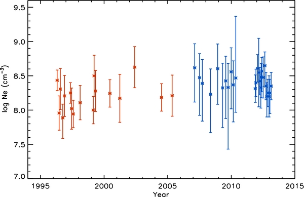
Figure 2. Coronal electron density measured with line intensity ratios from SUMER (red) and EIS (blue).
Download figure:
Standard image High-resolution image4.2. Thermal Structure
The DEM curves have been calculated for each data set, and the results are shown in Figure 3. The top panel of this figure displays a 2D plot, where the Y-axis corresponds to the ratio (in log scale) of the DEM curve to its peak value for each data set; the temperatures where the DEM reached its peak have been indicated by a white cross. DEM from different data sets have been placed side by side in temporal order so that the X-axis represents time from 1996 January 1. Only the 5.6 ⩽ log T ⩽ 6.7 temperature range has been displayed because, at larger or smaller temperatures, the DEM was negligible and/or too loosely constrained. The DEM curves were calculated using a Δlog T = 0.05 bin. The bottom panel of Figure 3 indicates the temperature of the DEM peak (stars) as well as the temperature range where the DEM curve is 1% or more of the peak value.
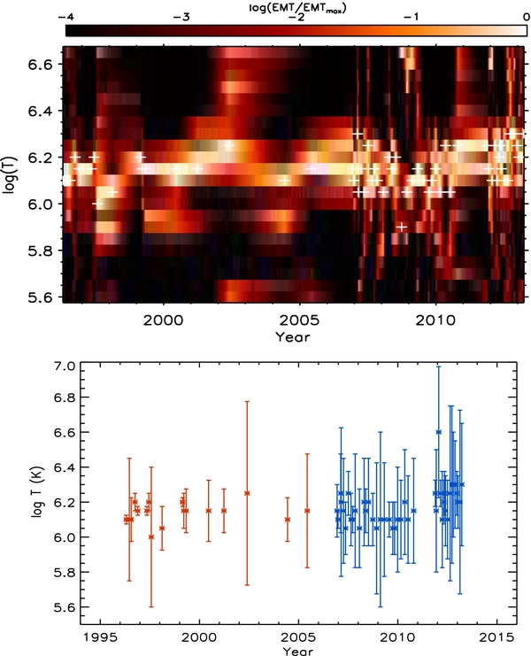
Figure 3. Top: temporal evolution of the thermal structure of off-disk streamers. For each time (corresponding to a data set) the Y-axis shows the ratio between the DEM to the value of its peak, in log scale. White crosses indicate the DEM peak. Bottom: plot of the temperature of the peak of each DEM (stars). Vertical bars represent the temperature ranges where the values of each DEM curve are 1% or more than the peak DEM value. Red and blue values were obtained with data from SUMER and EIS, respectively.
Download figure:
Standard image High-resolution imageFigure 3 shows a few important features. First, the plasma is not isothermal. Landi et al. (2012b) showed that even if the DEM technique indicates that the DEM is concentrated in a single temperature bin, the plasma is likely to be multithermal with a narrow temperature distribution. However, Figure 3 shows that the plasma thermal structure can have multiple peaks, have peaks that extend over multiple temperature bins, or high- and low-temperature tails.
Second, no clear trend can be seen of the DEM peak temperature with time; even if some variability in the peak temperature can be found from one data set to the next, overall, no systematic decline in streamer temperature like the one shown by in-situ data (Figure 1) can be found. This is especially important for the 2007–2010 period, where the anomalous minimum of cycle 23 was underway; this is where in-situ data show the deepest decrease in inferred coronal temperatures, and still, no clear indication of a decrease in streamer temperature can be seen. The temperature of the peak is in excellent agreement with estimates taken independently by a number of authors since the launch of SOHO (e.g., Warren 1999; Allen et al. 2000; Wilhelm et al. 2002; Landi & Feldman 2003; Parenti et al. 2003, see the review by Feldman & Landi 2008).
Third, significant high-temperature tails can occasionally be seen in a few DEM curves but there is no evidence of a steady, systematic presence of high- temperature plasma beyond the DEM peak. The same conclusion applies for cooler components of coronal hole-like plasma at the low temperature side of the DEM peak; even if several data sets show the presence of cold material, no secondary peak is constantly present.
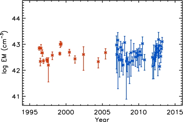
4.3. Total Emission Measure
The total EM, obtained by integrating the DEM over temperature, provides information about the total amount of material present along the line of sight. Even if it is dependent on the length of the line of sight and on the number of streamer structures that the latter crosses, it gives a rough idea of whether the total amount of plasma at the base of quiescent streamers has changed.
We have calculated the EM for each data set we have considered. Since the spectral line intensities in each data set were averaged over the entire area selected for analysis, the EM values have been corrected to account for the different pixel size and normalized to a 1'' ×1'' pixel. The EM is also dependent on the electron density, as it can be expressed as
Since the electron density is strongly dependent on distance from the limb, the EM values from data sets taken at different heights need to be normalized to the same height. We used the same procedure used to normalize the electron density. Results are shown in Figure 4 for the entire 1996–2013 period.
Figure 4. Temporal evolution of the total emission measure, obtained integrating the DEM shown in Figure 3. Red and blue values were obtained with data from SUMER and EIS, respectively.
Download figure:
Standard image High-resolution image
Uncertainties have been calculated from the uncertainties provided by the MCMC technique; their amplitude depends on the number of ions available in each data set. Since SUMER provided the largest number of ions, the uncertainties in the EM values it provides are usually lower. Figure 4 shows that total EM values can significantly change from one streamer to the next but no systematic dependence on the solar cycle is apparent.
Equation (4) also allows to make an estimate of the line of sight length, as L = EM/Ne2/A, where A is the area (in cm2) corresponding to a 1'' × 1'' pixel, if a unity filling factor is assumed and the electron density is interpreted as the average electron density along the line of sight. However, the uncertainties in the values of the total EM and of the electron density make such an estimate meaningless; a slight decreasing trend in L is washed away by the magnitude of the uncertainties.
5. DISCUSSION AND CONCLUSIONS
The measurements we have carried out on 60 different quiescent streamer data sets observed from early 1996 to early 2013 show that neither the electron density nor the electron temperature at their base experienced significant solar cycle related effects. Even considering some variability among different data sets, which are taken at different heights and in different positions within streamers, both these parameters seem to be stable throughout the full solar cycle 23 and the rising phase of cycle 24, despite the large differences in the level of activity shown by these cycles and the deep minimum that separates them. The first question that we need to ask is what relationship there is between the regions we have studied and the actual source regions of the slow solar wind.
There is still debate as to the origin of the slow wind within streamers, which in turn is related to the acceleration mechanism responsible for the wind generation. So far, two types of models of solar wind acceleration have been proposed: wave/turbulence-driven models and reconnection/loop opening models (Karachik & Pevtsov 2011 and references therein).
Wave-based models accelerate both types of wind from open magnetic field lines. Different field lines locations (e.g., deep inside coronal holes or at the boundary between coronal holes and streamers) and properties (expansion factor, heating location, and so on) dictate the characteristics of the wind that originates from them (Antiochos et al. 2012; Wang 2012 and references therein).
Reconnection-based models require the encounter of an open field line with a closed loop; reconnection causes the loop to open and release its material to the Heliosphere, while a new loop is generated from the open field line and one footpoint of the former loop. Different types of loops found in streamers and coronal holes account for different compositional characteristics of fast and slow solar wind. This mechanism, proposed by Fisk et al. (1999), Fisk & Schwadron (2001), and Fisk (2003), also predicts the diffusion of open field lines inside closed field regions, so that the slow wind can originate from regions inside streamers. However, Antiochos et al. (2012) proposed a model where reconnection can only occur at the boundary between coronal holes and streamers, with no diffusion of open field lines inside closed regions; like with wave-driven models, no slow wind can originate from inside closed field areas.
There are two more sources of the slow solar wind which have been proposed in the literature. First, reconnection near the top can cause large helmet streamer loops to release blobs of plasma into the heliosphere (e.g., Wang 2012 and references therein). These plasma ejections have been commonly observed in white light by SOHO/LASCO and SECCHI/COR 1 and COR 2, and originate at heights larger than 2 Rsun. Recently, Morgan et al. (2013) applied a new advanced image processing technique to LASCO white light images and identified a continuous expansion of active region closed field into the extended corona, made possible by the continuous rising of magnetic flux from the photosphere; they speculated that these rising structures constitute an additional component of the solar wind.
Our measurements of the properties of the base of streamers have direct relevance only to the reconnection-based slow wind acceleration scenarios proposed by Fisk and co-authors and to the closed field expansion scenario described by Morgan et al. (2013) since, in both cases, the slow wind is predicted to be made of plasma originally confined in closed field structures inside streamers. However, the constancy of the electron density and temperature values we measured in many different areas of the lowest portions of streamers seems to indicate that the thermodynamic properties of these structures, on the whole, do not change systematically with the solar cycle anywhere at low altitudes; in this case, also wave-driven models and coronal hole/streamer boundary reconnection models can be affected by our results.
The first consequence of our measurements is that the apparent decrease in coronal temperatures  as determined by the in-situ measurements of the O7 +/O6 + ratios is not primarily due to a net cooling of the solar corona, as suggested by von Steiger & Zurbuchen (2011), Kasper et al. (2012), and Lepri et al. (2013). Still, since O freezes in very close to the Sun, the causes of their changes need to be found at coronal heights comparable to those we considered in our own spectroscopic measurements. These changes can be due to three possible scenarios: changes in the streamer plasma properties at higher altitudes than observed in the present study, changes in the wind acceleration mechanisms, or a combination of both.
The mechanisms determining the charge state distribution of wind plasma are ionization and recombination due to ion–electron interactions. The effectiveness of both these processes depends linearly on the plasma electron density, while their collision rate coefficients depend on the electron temperature. Since charge states consistently decreased as solar cycle 23 headed toward the 2007–2010 minimum, there are two regions where the wind charge states could have been slanted toward lower values. The first one is the solar chromosphere and transition region. If the wind source region lies inside or below the chromosphere, and wind acceleration is more efficient in the transition region than in the corona, a faster wind would spend less time in these regions. In this case, transition region plasma would leave a more limited imprint in a faster wind's state of ionization; the latter would remain closer to the original, very low charge state distribution, and the subsequent crossing through the less dense and hotter solar corona would not leave enough time to the plasma to further ionize. Such a scenario is best applied to wave-driven models, such as those of Cranmer et al. (2007) and Oran et al. (2013), where waves extract, heat, and accelerate chromospheric plasma.
The degree of change to the charge state distribution of different elements can respond differently to variations in the acceleration mechanisms of the solar wind. In fact, Esser & Edgar (2000, 2001) carried out several studies to investigate the differences between the temperatures indicated by in-situ charge state ratios and spectroscopic determinations. They found that several processes could cause the observed discrepancies, although in-situ measurements alone were not able to provide enough constraints to discriminate among them. Most notably, Esser & Edgar (2000, 2001) indicated the presence of non-Maxwellian distributions of electrons and of differential flows of ions of the same element as possible mechanisms that can affect charge state ratios. The results of these authors can be applied to the discrepancy between the results of the present paper and the in-situ measurements of charge state ratios. In this scenario, changes in wind acceleration related to the solar cycle can affect the flows of different elements and different ions of the same element to different degrees, resulting in mixed variations in the frozen-in charge state ratios within the same type of plasma, consistent with the in-situ measurements of Lepri et al. (2013).
Reconnection-based models imply that the slow solar wind plasma is initially confined in closed magnetic loops and is released in the heliosphere following a reconnection event that opens the host structure. Under this scenario, a possible cause for a decrease of charge state ratios is an increase in the electron density in the outer layers of the solar corona beyond the SUMER and EIS field of views relative to the values at the beginning of the solar cycle. Such an increase can be obtained with an increase in the density scale height. In fact, the solar wind charge state composition in the source region has already reached equilibrium at coronal temperatures inside closed magnetic loops before reconnection allows them to release their plasma in the heliosphere. Once this plasma is accelerated outward, it crosses a medium whose electron temperature decreases from the values of the coronal sources. A larger electron density in the outer corona would increase the recombination of coronal ions into less ionized species and decrease the overall charge state distribution. A decreased wind acceleration in these regions would also provide the same result, by increasing the time that the wind plasma spends in these colder regions.
In both cases, a cycle-dependent effectiveness of wind acceleration at the beginning of the wind trajectory needs to be compensated at greater distances, since in-situ measurements of the slow wind velocity do not show any significant solar cycle dependence.
The discrepancy between spectroscopic and in-situ coronal temperature measurements can also be explained by the third scenario, where the slow wind originates from the streamer cusp (Kohl et al. 2006 and references therein). In this case, the wind charge state composition is likely not affected by the measured plasma conditions in the inner corona, and its distribution is only determined by the conditions in the outer solar corona.
If the slow solar wind originates from the expanding closed field structures observed by Morgan et al. (2013), the solar cycle effects on the rising plasma need to take place at larger heights than those considered in the present work. Since the plasma remains confined in closed structures up to large altitudes where the ambient plasma density is very low, changes in the slow wind composition need to take place while the plasma is still confined, likely due to a decrease of the loop plasma temperature not measured at low altitudes.
It is not yet possible to discriminate among such scenarios. The present work represents only a first step in understanding the causes of the evolution of the in-situ wind properties because the limited field of view of high-resolution spectrometers prevented a detailed study of the properties of an entire streamer and further restrict our results to the innermost regions in the solar corona, where the signal-to-noise ratios are largest. We could only conclude that the properties of the coronal base of streamers do not change systematically along 17 yr. Despite this, changes might take place at larger altitudes than we observe. Also, this study covers 17 yr of solar observations, and it needs to be prolonged both to future observations as they will become available and extended to earlier dates than SOHO. We plan to investigate the thermal structure of large scale streamers using observations from SOHO/EIT, STEREO/EUVI, and SDO/AIA in a future work.
The work of E.L. was supported by NASA grant NNX11AC20G; the work of P.T. is supported by NASA grants NNX11AC20G and NNX10AF29G. We thank the referee for very useful comments that helped improve the original manuscript.