
ABSTRACT
The acceleration of suprathermal charged particles in the heliosphere under pressure balance conditions including for the first time the radial spatial particle diffusion and convection in the solar wind is investigated. The physical conditions are derived for which the stationary phase space distribution of suprathermal particles approaches the power-law distribution f∝p−5, which is often seen in spacecraft observations. For separable source distributions in momentum and position we analytically solve the stationary particle transport equation for a radially constant solar wind speed V0 and a momentum-independent radial spatial diffusion coefficient. The resulting stationary solution at any position within the finite heliosphere is the superposition of an infinite sum of power laws in momentum below and above the (assumed mono-momentum) injection momentum pI. The smallest spatial eigenvalue determines the flattest power law, to which the full stationary solution approaches at large and small enough momenta. Only for the case of a reflecting inner and a free-escape outer spatial boundary, does one small eigenvalue exist, yielding the power-law distribution f∝p−5 at sufficiently large momentum values. The other three spatial boundary conditions imply steeper momentum spectra. Momentum spectra and radial profiles of suprathermal particles are calculated by adopting a uniform outer ring spatial source distribution.
Export citation and abstract BibTeX RIS
1. INTRODUCTION
In interplanetary space, there is always a significant population of particles with energies greater than a few times the solar wind thermal energy, where we normally expect very little flux if the particles have a Maxwellian distribution. These suprathermal particles (STPs) form a power-law tail in the energy spectrum. Observed spectra obtained by spacecraft in various regions of the heliosphere often possess a spectral slope corresponding to an isotropic phase space distribution function f∝p−5, which Fisk & Gloeckler (2006, 2008) called a universal or common spectrum.
The source of these particles is not completely certain (Mewaldt et al. 2005). Some may come from the solar corona, but one most noticeable suprathermal component is the pickup ions. These are originally neutral atoms, mostly interstellar neutrals, penetrating through heliospheric magnetic fields into the inner heliosphere, where they are ionized by solar UV radiation or through charge exchange with the solar wind ions. The newly born pickup ions have almost zero speed in the initial reference frame and they immediately have to convect with the outgoing solar wind plasma with an embedded magnetic field. The initial speed of these pickup ions in the plasma reference frame is then equal to the solar wind speed. Subsequent rapid pitch-angle scattering by magnetic turbulence makes them an isotropic shell distribution with a steep cutoff at exactly the local solar wind speed in the plasma reference frame. Observations in interplanetary space (Gloeckler et al. 1994) often show that pickup ions can extend to much higher speeds. Clearly, they are accelerated in the interplanetary space. Similarly, one can also argue that STPs of solar or other origins should also undergo acceleration during their transport through interplanetary space.
The mechanism for the acceleration of STPs is still under debate. A few authors suggested that interplanetary shocks can accelerate pickup ions and other SPTs (e.g., Giacalone et al. 1997), but most scientists attribute the acceleration of these particles to a stochastic mechanism in the form of diffusion in momentum space by more ubiquitous electromagnetic waves or turbulence in the solar wind plasma (Isenberg, 1987; Schwadron et al. 1996; Le Roux & Ptuskin 1998; Chalov et al. 2004, 2006). Because of the observed near isotropy of the STP distribution function, it is generally accepted that the STPs are scattered in low-frequency magnetohydrodynamic (MHD) turbulence well below the nonrelativistic proton cyclotron frequency. Faraday's induction law then implies that the ratio of the electric and magnetic field strengths of MHD turbulence is given by  (with Alfvén velocity VA), which in interplanetary space is well below unity. In situ electric field fluctuation measurements in the solar wind (e.g., Bale et al. 2005) confirm that
  . These small fluctuating electric fields in the wave and turbulence can accelerate or decelerate STPs randomly, depending on the relative direction between wave variation and particle motion.
In the diffusion approximation, one can establish that the particle's momentum distribution obeys the diffusion–convection transport equation, containing both spatial and momentum diffusion and convection terms. Spatial and momentum diffusion can be directly established in the perturbative quasilinear theory (Skilling 1975; Schlickeiser 1989, 2002), but other nonlinear theories can also arrive at diffusive transport (e.g., Qin et al. 2002; Zhang 2010). It has been argued that the quasilinear approximation holds in the interplanetary medium despite the fact that interplanetary turbulence observation indicates that the turbulent magnetic field has the same strength as the ordered uniform (on scales of the particles' gyroradii) background magnetic field. The underlying reason is that most of the magnetic turbulence (about 85% according to Bieber et al. 1996) is in the form of axisymmetric transverse two-dimensional (2D) turbulence that contributes very little to particle scattering (Shalchi & Schlickeiser 2004). However, the transverse 2D turbulence is responsible for efficient wandering of magnetic field lines (see Section 2.1). For the remaining 15% magnitude turbulence, predominantly in the form of slab turbulence, the ratio δBslab/B0 is considerably less than unity, fulfilling the quasilinear approximation condition. As an aside we note that the proper diffusion approximation to the Fokker–Planck transport equation (Schlickeiser 1988, 1989; Schlickeiser et al. 1991, 2010), taking into account finite frequency effects of forward and backward moving MHD waves, avoids the earlier claimed 90° scattering problem. In the presence of MHD turbulence (such as Alfvén or magnetosonic waves), the momentum diffusion coefficient is always tied to the particle's pitch-angle diffusion coefficient or parallel spatial diffusion coefficient. Chalov et al. (2004, 2006) considered wave generation of particle acceleration in a self-consistent manner. They found that the amount of acceleration of the pickup ions by Alfvén or magnetosonic turbulence in the interplanetary space is not enough to overcome the adiabatic cooling of particles in the expanding solar wind and produce a significant power tail beyond the initial solar wind speed.
Stochastic acceleration of charged particles can also occur when the particles go through a magnetic medium undergoing random compression or expansion. In this mechanism it is the large-scale convective electric field that accelerates or decelerates particles in a random manner. This case has been investigated by Bykov & Toptygin (1982, 1993) and later Ptuskin (1988), who derive a diffusion equation in the momentum space using a quasilinear method with an additional ensemble average over velocity fluctuations. Ptuskin (1988) studied a case in which the particle diffusion is much too large compared to the characteristic distance between consecutive regions of plasma compression or expansion and he dismissed this mechanism as an important acceleration mechanism for cosmic rays in the interstellar medium.
Recently, observation of the common f∝p−5 spectrum as drawn renewed attention to the mechanism of particle acceleration by random compressions of large-scale plasma motion. Fisk & Gloeckler (2006, 2008) and Fisk et al. (2010) suggested that this acceleration mechanism can automatically produce the f∝p−5 spectrum, but the calculation by Jokipii & Lee (2010) disagreed. Zhang (2010) took a different approach to this problem. Instead of the quasilinear approximation, he solved the Parker transport equation for particles moving through a train of compressible waves. Although a special form of the wave trains is prescribed in the model, it is found that acceleration of particles can be very fast if the particle diffusion length is greater than the size of plasma compression region but smaller than the length of the wave train. The behavior of particle acceleration is similar to diffusion in the momentum space, but with a momentum diffusion coefficient D∝p2. This mechanism, if we let it go on without significant adiabatic cooling, will soon establish a f∝p−3 spectrum. Such a distribution function contains too much energy or pressure. Zhang (2010) and Zhang & Lee (2011) argued that the pressure built up by the accelerated particles can modify the amplitude of the plasma compression waves, such that the rates of particle acceleration by the plasma compressions and adiabatic cooling are equal. At that point, a f∝p−5-distribution is established, independent of the details of wave or particle parameters as long as the rate of particle acceleration decreases with total particle pressure.
The derivation of the f∝p−5 spectrum in Zhang (2010) and Zhang & Lee (2011) is done in the reference frame of the particles and the intensity of particles has reached a uniform spatial distribution. This assumption may not be true on the scale size of the heliosphere as the rate of adiabatic cooling of particles and the particle diffusion coefficients could depend on the radial distance from the Sun so that the particle intensity is not uniform. It is the purpose of this paper to explore the spectrum of accelerated pickup ions or STPs in a more realistic condition of particle transport in the heliosphere. We show that the f∝p−5 spectrum can be established under some plausible conditions of particle transport properties and plasma wave environment, as long as the pressure of accelerated particles has reached a level that is able to force plasma waves to reach the balance between particle acceleration and adiabatic cooling.
2. BASIC EQUATIONS
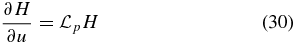
Stochastic particle acceleration in cosmic sources occurs in the presence of multiple small-scale turbulent MHD plasma waves propagating in different directions (Zhang & Lee 2011). Its efficiency is characterized by a momentum diffusion coefficient D that is closely related to particle pitch-angle scattering, which causes parallel spatial diffusion along the ordered guide magnetic field, described by the parallel spatial diffusion coefficient κ∥ (Schlickeiser 1989). The general relation

holds, where the constant g depends on the nature and geometry of the plasma waves, and has been determined before for the case of parallel propagating shear Alfvén waves (Dung & Schlickeiser 1990) with an additional contribution from isotropically distributed fast magnetosonic waves (Schlickeiser & Miller 1998).
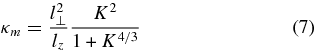
Recently, Zhang & Lee (2011) demonstrated that in the case of random fluctuations of the large-scale plasma flow (Bykov & Toptygin 1993; Ptuskin 1988; Jokipii & Lee 2010), maximum stochastic acceleration occurs with different momentum and spatial diffusion coefficient:
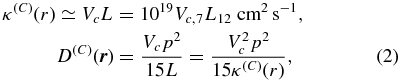
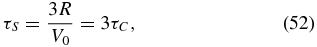
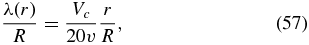
where L = 1012L12 cm is the characteristic length of the plasma velocity variations and Vc = 107Vc, 7 cm s−1 is the speed of compression waves, which is not necessarily the Alfvén speed. L12 and Vc, 7 are scaling factors, accounting for deviations from the most likely values L12 = 1 and Vc, 7 = 1. κ(C)(r) is the particle spatial diffusion coefficient along the propagation direction of the compression waves.
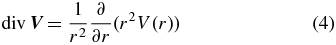
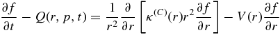
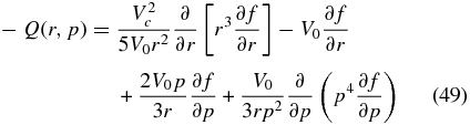
Ignoring drifts in non-uniform or curved guide magnetic fields, the isotropic part of the distribution function f(r, p, t) of the energetic particles in spherical position coordinates then obeys the radial diffusion–convection transport equation:
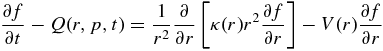
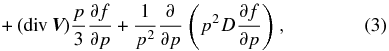
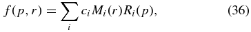
where Q(r, p, t) describes sources and sinks of particles,
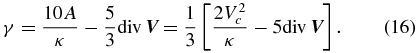
in radial flow such as the solar wind, and

2.1. Radial Spatial Diffusion
The radial spatial diffusion coefficient in the transport equation (3)

is determined by the respective contributions of the parallel, perpendicular, and compressional spatial diffusion coefficients, respectively. Here, ψ(r) denotes the angle of the background Parker spiral magnetic field with respect to the radial direction, which in the outer heliosphere is near π/2. In Equation (6) we assume that the compression waves propagate predominantly along the radial solar wind direction.3 In the outer heliosphere (the likely source of pickup ions) the radial diffusion coefficient is determined predominantly by the perpendicular spatial diffusion coefficient κ⊥(r) and the compressional contribution κ(C).
In the absence of drifts in non-uniform or curved guide magnetic fields, due to their small gyroradii the perpendicular spatial diffusion of SPTs is dominated by magnetic field line random walk from the transverse 2D magnetic turbulence. The magnetic diffusion coefficient is given by (Bian et al. 2011; Hauff et al. 2010)
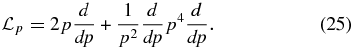
in terms of the Kubo number (Kubo 1963; Vlad et al. 1998; Zimbardo et al. 2000)
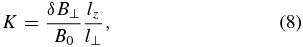
where lz and l⊥ are, respectively, the parallel and perpendicular auto correlation lengths of the fluctuating slab and 2D magnetic field components. Expression (7) interpolates between the quasilinear (K ≪ 1) and percolation trapping (K ≫ 1) regions of magnetic field transport. Satellite observations find that the large-scale solar wind fluctuations are nearly isotropic lz ∼ l⊥ ∼ 106 km (Tu & Marsch 1995), implying interplanetary Kubo numbers of K = 0.85 for δBperp/B0 = 0.85. In the small gyroradius limit, as appropriate for STPs, the particle perpendicular spatial diffusion coefficient is given by (Jokipii 1966; Rechester & Rosenbluth 1978; Bitane et al. 2010)
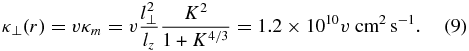
Compared to the compressional contribution κ(C) given in Equation (2), the field line random walk contribution (9) is negligibly small for STP velocities smaller than v = 104L12Vc, 7 km s−1, which is well fulfilled for pickup ions adopting the likely values L12 = Vc, 7 = 1.
2.2. Radial Transport Equation
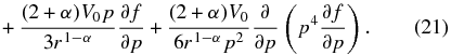
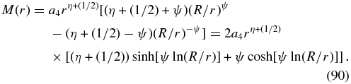
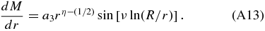
Moreover, we assume that the momentum diffusion coefficient (5) is dominated by the contribution from compressional waves  given in Equation (2). The STP transport equation (3) then reads
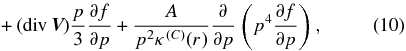
with the constant

As we shall demonstrate in the following, these choices for the radial and momentum diffusion naturally account for the formation of power-law momentum distribution functions of STP as observed. It is straightforward to see that any other choice with momentum-dependent spatial diffusion coefficients will lead to non-power-law STP momentum distributions as solutions of the transport equation (10), which are not observed. The observed momentum power laws of SPT already point to the required microphysical processes causing momentum diffusion and radial spatial diffusion in the outer heliosphere.
2.3. Pressure Balance
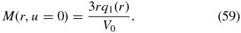
For suprathermal charged particles the nonrelativistic treatment of Zhang & Lee (2011) is appropriate. Following their approach we introduce the pressure of energetic particles
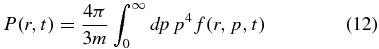
and consider a uniform (in space and time) source injecting mono-energetic particles, i.e.,

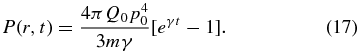
Multiplying Equation (3) by 4πp4/3m and integrating over all momenta, we obtain for the total change of pressure (from now on we will drop the index (C) and identify κ = κ(C))
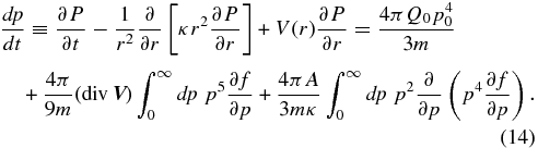
Integrating the two last terms with respect to p by parts, with the use of f(r, p = 0, t) = f(r, p = ∞, t) = 0, then provides

with
Equation (15) can be readily integrated over time, yielding with P(t = 0) = 0
It was noted by Zhang & Lee (2011) that for γ > 0, in the presence of a large enough initial stochastic acceleration, the pressure in energetic particles (17) becomes infinitely large as t → ∞. In order to avoid such singular behavior they argue that it is necessary to require γ = 0 for a steady-state system, to which we refer as pressure balance condition
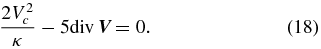
This pressure balance condition is achieved by limiting the particle scattering and acceleration rates through a nonlinear feedback mechanism of particle pressure on plasma waves.
In spherical flows with

with V0 = constant and α ∈ [0, 1), this provides a radially increasing spatial diffusion coefficient of the form

Such a radial variation of the spatial diffusion coefficient is quite reasonable in the heliospheric magnetic field as the inferred radial dependences κ(r)∝rξ with ξ ∈ [1.1, 1.4] from the intensities of galactic and anomalous cosmic rays (Fujii & McDonald 2005) indicate.
2.4. Particle Transport Under Pressure Balance Condition
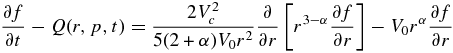
The radial particle transport equation (10) under the pressure balance condition (20) then reads
Zhang & Lee (2011) have solved a spatially non-diffusive transport equation for the particles for the case of a constant solar wind velocity (α = 0), demonstrating that due to the pressure balance coupling of momentum diffusion and adiabatic deceleration, the particle distribution at large momenta settles with a distribution f(p)∝p−5, which is commonly seen in STP (Fisk & Gloeckler 2006, 2008). While the spatial diffusion can be neglected for very low energy particles in the region where its density variation is small within the particle diffusion length, here we extend our study to include stationary solutions of the full spatially dependent transport equation (21) to investigate the influence of the spatially increasing spatial diffusion coefficient (20) on the momentum spectrum of accelerated particles under pressure balance conditions. Because the spatial diffusion coefficient increases with radial distance and particle energy, its effect cannot be ignored at large enough radii r and momentum p.
3. SOLUTION OF THE STATIONARY TRANSPORT EQUATION
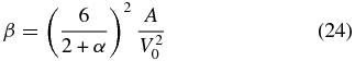
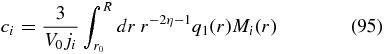
For separable source distributions Q(r, p) = q1(r)q2(p) the stationary transport equation under pressure balance condition is
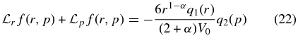
with the momentum-independent spatial operator
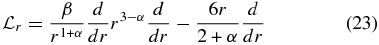
with the constant
and the position-independent momentum operator
The operators  and
and  can be understood as the rate of particle transport in r and p, respectively, normalized by half the rate of adiabatic cooling
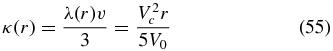
 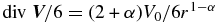 .
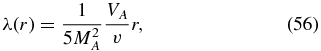
.
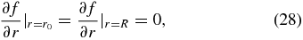
As momentum boundary conditions we use finiteness at p → 0 and vanishing particle density as p → ∞, i.e.,

As spatial boundary condition we use either free-escape at the inner (r0) and outer (R) radii, i.e.,

or reflecting boundary conditions at r0 and R, i.e.,
respectively.
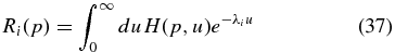
According to the scattering time method (Wang & Schlickeiser 1987; Schlickeiser 2002, Ch. 14), Equation (22) is solved by the convolution
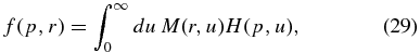
where H(p,u) satisfies the momentum boundary conditions (26) and
with

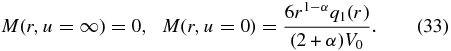
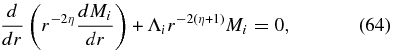
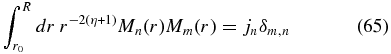
The age distribution M(r, u) satisfies the spatial boundary conditions (27) and

with
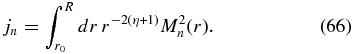
3.1. Leaky-box Equations
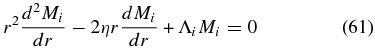
The spatial operator (23) is of Sturm–Liouville form and thus has the complete eigenfunction system Mi(r). The age distribution M(r, u) then can be expanded in this orthonormal system as
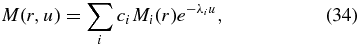
where λi denotes the real eigenvalues of the spatial operator, being determined by the spatial boundary conditions (27), and the coefficients ci have to be calculated from the initial condition (33) using orthonormality relations of Mi:
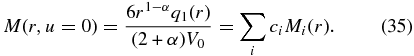
Inserting the expansion (34) into the convolution (29) leads to
where each of the functions (see Schlickeiser 2002, Ch. 14.3.2)
obeys the leaky-box equations:

Equation (36) indicates that the steady-state solution M(r, u) can be expressed as a (infinite) sum of products of the functions Ri(p) and ciMi(r). Each function Ri(p) satisfies a leaky-box equation (38), where the corresponding spatial eigenvalues λi enter in the form of a catastrophic escape loss rate.
3.2. Solution of the Leaky-box Equations
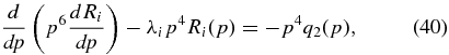
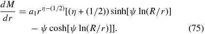
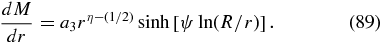
Inserting the momentum operator (25) then provides for the leaky-box equation (38):

The self-adjoint form of this equation reads
which for arbitrary injection spectra q2(p) is solved by
The Green's function G(p, p0) obeys
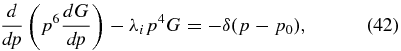
and with the momentum boundary condition (26) is given by
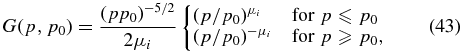
with

Inserting the Green's function (43) into Equation (41) we find
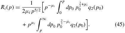
In the case of a mono-energetic injection q2(p0) = Q0δ(p − pI), we readily find the broken power-law solution:
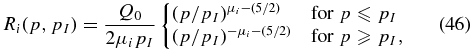
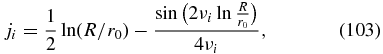
so that the spectral index of accelerated particles  with momentum p ⩾ pi is given by
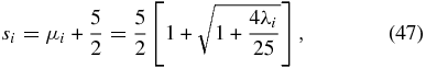
which approaches the value si = 5 from above, provided that the spatial eigenvalues or escape loss rates λi ≪ (25/4) = 6.25 are much smaller than the critical value 6.25. If such small eigenvalues are possible, a suitable explanation of the common p−5-momentum spectrum has been established.
3.3. Interlude
Equations (36), (45), and (46) represent the full formal solution of the stationary particle transport equation for arbitrary separable particle source distributions and general radial solar wind variations of the form (19). The resulting solution is the superposition of an infinite number of momentum power-law distributions, whose spectral indices are determined by the eigenvalues λn of the spatial propagation equation. Each power-law contribution is weighted by the respective expansion coefficient cn, depending on the spatial source distribution of STPs. The power law resulting from the smallest spatial eigenvalue λ1 will dominate the solution at sufficiently high-momentum values because the spectral indices from the contribution of larger spatial eigenvalues will be greater than s1.
The determination of the eigenvalues λn and the expansion coefficients cn require solving the eigenequation

subject to the spatial boundary conditions (27) and/or (28).
Throughout this work we restrict our analysis to the case of a constant solar wind velocity (α = 0), whereas radially varying solar wind velocities will be investigated in future work. As we will demonstrate, the case of a constant solar wind velocity allows us the full analytic calculation of the eigenvalues and the expansion coefficients.
In particular, we will investigate the influence of the chosen spatial boundary conditions on the eigenvalues and thus on the power-law spectral indices of the accelerated STPs. Of particular interest is the calculation of the smallest possible eigenvalue λ1 for different spatial boundary conditions, which is considered in Section 5. If this is much smaller than the value 6.25, the high-momentum spectrum of accelerated particles equals the p−5-spectrum.
In the following we investigate the solution of the eigenequation (48) for the constant solar wind velocity case under four different spatial boundary conditions:
(1) free-escape boundary conditions Mn(r0) = Mn(R) = 0 at the inner (r0) and (R) and outer radii;
(2) reflecting boundary conditions  at the inner and outer radii;
(3) inner free-escape (Mn(r0) = 0) and outer reflecting ((dMn/dr)R = 0) boundary conditions; and
(4) inner reflecting ( ) and outer free-escape (Mn(R) = 0) boundary conditions.
The boundary conditions in case D closely represent the real boundary conditions of the heliosphere. At the inner boundary, the magnetic field is strong, so the majority of particles coming in from the outer heliosphere are mirrored back, suggesting that a reflective boundary would be most appropriate. At large radial distances, the magnetic field is too weak to contain these particles and the radial geometry also dilutes the particle density, making an escape boundary most likely.
4. SPATIAL PROBLEM FOR CONSTANT SOLAR WIND SPEED α = 0
For constant solar wind speed (α = 0) the steady-state transport equation (21)
is controlled by the four closely related timescales for
(1) spatial convection

(2) adiabatic deceleration
(3) stochastic acceleration
and (4) spatial diffusion

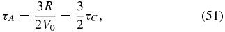
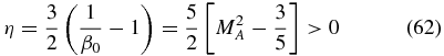
with the constant
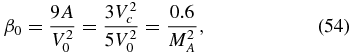
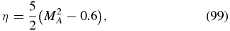
where MA = V0/Vc is the Mach number of the solar wind speed. The parameter β0, determined by the Mach number of the solar wind speed, therefore has the strongest influence on the resulting particle spectrum f(p, r). τD is longer than τC in the supersonic wind, but these timescales can be comparable in the subsonic wind. This makes the spatial diffusion important in the outer heliosphere, particularly in the heliosheath.
For the case of a constant solar wind speed α = 0, the radial spatial diffusion coefficient
implies the radially increasing scattering mean free path
which for an adopted Mach number MA = 2 yields the small ratio
so that for all STPs with velocities v ≫ 0.05 Vc the spatial diffusion approximation is justified.
Moreover, for a constant solar wind speed α = 0, the spatial operator (23) reads

The initial condition (33) becomes
With the ansatz (34) for the age distribution the eigenfunctions obey the eigenequation:

or
with
and

4.1. Self-adjoint Form
The self-adjoint form of the eigenequation (61) reads
providing with the boundary conditions (27)–(28) the orthonormality relations
with
4.2. Normal Form
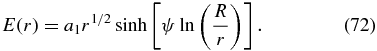
With Mi(r) = rηE(r) the normal form of Equation (61) reads
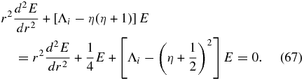
Equation (67) is readily solved by E(r)∝rk with
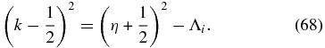
Obviously, for each specified boundary conditions (A)–(D), we have to consider the two cases of (1) small eigenvalues Λi < (η + (1/2))2, corresponding to λi < β0[η + (1/2)]2, and (2) large eigenvalues Λi < (η + (1/2))2, corresponding to λi ⩾ β0[η + (1/2)]2. The first case is particularly important because it implies the p−5-spectrum at high momenta if the smallest eigenvalue λ1 is much smaller than 6.25. We consider each case in turn in the next section and in the Appendix, respectively.
5. SMALL EIGENVALUES λi < (η + (1/2))2
In this case we set

Equation (68) then provides

5.1. Cases A and D
The free-escape boundary condition at r = R gives

so that
5.1.1. Case A
The free-escape condition at the inner boundary E(r0) = 0 in this case then demands

providing as the only possibility ψ = 0, which implies according to Equation (72) the unusable trivial solution Ei(r) = 0. Therefore, in this case of the boundary conditions no small eigenvalue Λi exists.
5.1.2. Case D
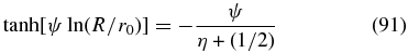
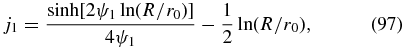
The solution (72) implies

yielding
The inner reflecting boundary conditions  in this case then provide the condition

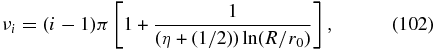
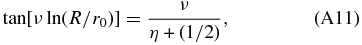
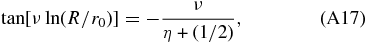
for the smallest first eigenvalue Λ1 in this case. For ψ > η + (1/2), no solutions of Equation (76) exist, because the tanh function is limited to values less than unity. Consequently, the value of ψ has to be smaller than η + (1/2), which according to Equation (69) implies that the eigenvalue Λ1 is nonnegative.
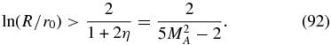
Moreover, for a nontrivial solution of the transcendental equation (76) the slope ln (R/r0) of the tanh function at ψ = 0 has to be larger than the slope (1/(1/2) + η) of the line (2ψ/1 + 2η), i.e.,
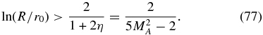
We therefore find for this boundary condition case one small eigenvalue Λ1, provided that Equation (77) is fulfilled.
With y0 = ln (R/r0) and K = ψy0 we can write Equation (76) as
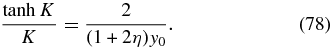
For values of
the solution of Equation (78) can be approximated as

with

yielding

Equation (80) then becomes

With the definition of K = ψy0 we obtain as the only small solution of the transcendental equation (76)

Combination with Equation (69) then provides for the small eigenvalue
Equations (63) and (54) then yield

which for large R ≫ r0 and Mach numbers MA > 1 is small compared to unity.
The expansion coefficient a1 can be determined by using the orthonormality property of M1(r), i.e.,

5.2. Cases B and C
The solution (70) implies

so that the outer reflecting boundary condition (dM/dr)R = 0 in cases B and C yields
5.2.1. Case B
The inner reflecting boundary condition  in this case then can only be fulfilled for ψ = 0, so that no small eigenvalues with nontrivial solutions exist in this case either.
5.2.2. Case C
The outer reflecting boundary condition (dM/dR)R = 0 implies for the solution (88)
The inner free-escape condition M(r0) = 0 then provides the condition
with the only solution ψ = 0. Also in this case of boundary conditions no small eigenvalue with nontrivial eigensolution exists.
5.3. Interlude
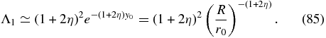
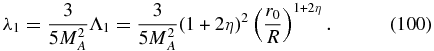
As the most important result of this section we found that the spatial boundary condition D (reflecting inner and free-escape outer boundary) is the only case where a small eigenvalue is possible, provided that
The eigenvalue is then given by
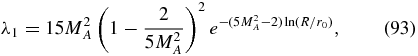
which for large R ≫ r0 and Mach numbers MA > 1 is small compared to unity and to the value 6.25. This mode gives a negligible particle escape loss.
For completeness we consider in Appendix the case of large eigenvalues Λi ⩾ (η + (1/2))2.
6. FULL SOLUTION OF THE STATIONARY TRANSPORT EQUATION FOR α = 0 AND REFLECTING INNER AND FREE-ESCAPE OUTER BOUNDARY
6.1. Collection of Earlier Results
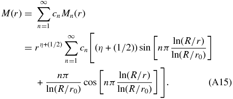
According to Equations (36) and (46) the full stationary solution for α = 0 and mono-energetic injection with rate Q0 at momentum pI reads

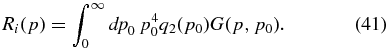
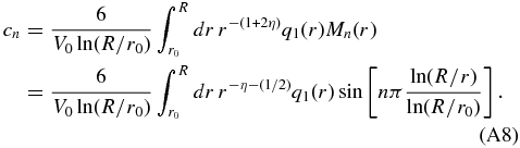
with the step function H(x) = (1 + (x/|x|))/2. For arbitrary spatial source distributions q1(r), the expansion coefficients are given by
with

For an inner reflecting (at r0) and outer (at R) free-escape boundary condition, we found

with
and
Likewise, for i ⩾ 2

with
so that
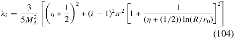
and
6.2. Illustrative Choice of Parameters
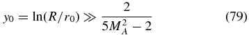
In the slow solar wind we adopt the Mach number MA = 1.35, implying the parameter value η = 3.056. This small Mach number should be regarded as a best-fit value and it corresponds to rather strong velocity fluctuations. For higher values of MA we obtain much too small values of the first expansion coefficient a1 compared to the others ai, i ⩾ 2, so that the momentum spectrum of accelerated STPs approaches the p−5-power-law spectrum (shown in Figures 1 and 3) at particle momenta that are too high. Condition (79) for the existence of a small eigenvalue then demands

which is well fulfilled for our adopted values R = 10r0.

Figure 1. Momentum distribution of accelerated suprathermal particles inside (at r = 0.7R) of the adopted uniform outer ring (from 0.5R to 0.9R) spatial source distribution for a constant solar wind speed with an inner (at r = 0.1R) reflecting and an outer (at R) free-escape boundary condition.
Download figure:
Standard image High-resolution imageIn Table 1 we calculate the first five spatial eigenvalues λi and the associated power-law spectral indices μi(λi). The first extremely small eigenvalue Λ1 implies μ1 = 2.5, whereas the higher eigenvalues yield steeper spectral index values μi > 3.8.
6.3. Expansion Coefficients
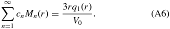
Guided by more exact determinations (Zhang & Schlickeiser 2012) we approximate the spatial radial distribution of injected particles as a uniform outer ring distribution:

with r1 = 0.5R and r2 = 0.9R. It is convenient to scale these expansion coefficients as
with the dimensionless values
With Equation (94) we then obtain for the full stationary solution for α = 0 and mono-energetic injection with rate Q0 at momentum pI

with

With the spatial source distribution (107) we then obtain for the first expansion coefficient:

For i ⩾ 2 we derive
In the last column of Table 1 we calculate the first five expansion coefficients ai.
The stationary solution (110) for α = 0 and mono-energetic injection with rate Q0 at momentum pI finally reads

In Figures 1 and 2, we show the momentum spectra of the accelerated STPs inside (r = 0.7R) and outside (r = 0.1R) of the adopted spatial source distribution. In each plot we show the total momentum distribution and the contribution from the higher eigenvalues i ⩾ 2. The momentum spectra are flat below pi. Immediately above pi, due to the influence of higher-order eigenfunctions, they exhibit a slight falloff, until at large enough momenta they flatten toward the p−5-spectrum. This is best visible in Figure 2.
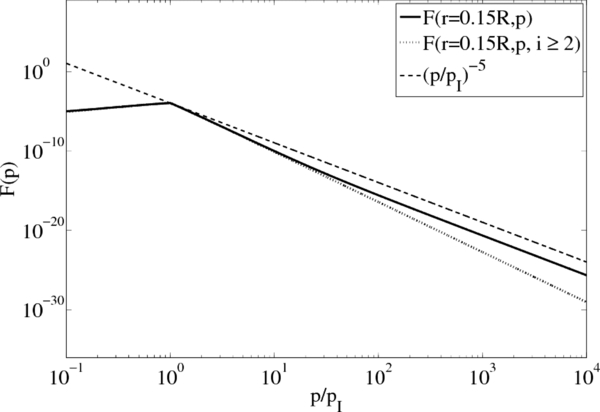
Figure 2. Same as Figure 1 outside (r = 0.15R) of the outer ring spatial source distribution.
Download figure:
Standard image High-resolution imageThe radial profile of the accelerated STPs at p = 4pI and p = 10pI shown in Figures 3 and 4, respectively, first decreases because of the reflecting boundary condition at r = 0.1R, before they increase significantly at r ⩾ 0.4R toward the outer ring source distribution. At small radial distances the radial profile suffices a bit from the well-known mathematical Gibbs phenomenon of Fourier series expansion (Carslaw 1950, Ch. 9), providing negative particle densities as we have truncated the sum over i in Equation (114) at i = 10. This mathematical problem can be easily alleviated by modifying the radial boundary conditions requiring constants values M(r0) = M(R) = c0 at the edges and additionally  . The profile in Figure 2 should therefore be regarded as the relative radial variation of accelerated STPs.
Table 1. The Spatial Eigenvalues λi, Spectral Indices μi, and Dimensionless Expansion Coefficients ai for η = 3.056 (MA = 1.35) and R = 10r0
| i | λi | μi | ai |
|---|---|---|---|
| 1 | 1.29 × 10 −6 | 2.5 | 1.17 × 10 −5 |
| 2 | 8.26 | 3.80 | 1.27 |
| 3 | 20.53 | 5.16 | −0.28 |
| 4 | 40.99 | 6.84 | −0.11 |
| 5 | 69.63 | 8.67 | 0.30 |
| 6 | 106.45 | 10.56 | −0.31 |
| 7 | 151.45 | 12.49 | 0.11 |
| 8 | 204.64 | 14.44 | −0.03 |
| 9 | 266.01 | 16.41 | −0.17 |
| 10 | 335.56 | 18.38 | 0.13 |
Download table as: ASCIITypeset image
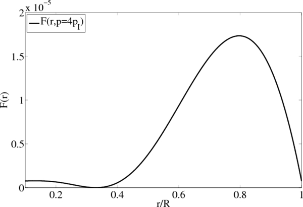
Figure 3. Radial distribution of accelerated suprathermal particles with momentum p = 4pi for the adopted uniform outer ring (from 0.5R to 0.9R) spatial source distribution, a constant solar wind speed, and an inner (at r = 0.1R) reflecting and an outer (at R) free-escape boundary condition.
Download figure:
Standard image High-resolution image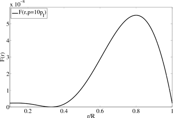
Figure 4. Radial distribution of accelerated suprathermal particles with momentum p = 10pi for the adopted uniform outer ring (from 0.5R to 0.9R) spatial source distribution, a constant solar wind speed, and an inner (at r = 0.1R) reflecting and an outer (at R) free-escape boundary condition.
Download figure:
Standard image High-resolution image
7. SUMMARY AND CONCLUSIONS
We explored the acceleration of suprathermal charged particles in the heliosphere under pressure balance conditions including for the first time the radial spatial particle diffusion and convection in the solar wind. In particular, we were interested in deriving the physical conditions for which the stationary phase space distribution of STPs approaches the power-law distribution f∝p−5, often seen in spacecraft observations. We first showed that power-law momentum distributions only result if the radial spatial diffusion and the momentum diffusion of particles are caused by the contributions from compressional waves. Inclusions of other momentum-dependent spatial diffusion coefficients will lead to non-power-law STP momentum distributions, which are not observed.
For separable source distributions in momentum and position we analytically solved the stationary particle transport equation for a radially constant solar wind speed V0 and a momentum-independent radial spatial diffusion coefficient, by expanding the solution in terms of the eigenfunctions of the spatial operator. For either reflecting or free-escape spatial boundary conditions, these spatial eigenfunctions form a complete orthonormal basis. We demonstrated that the resulting stationary solution at any position within the finite heliosphere is the superposition of an infinite sum of power laws in momentum below and above the (assumed mono-momentum) injection momentum pI. The smallest spatial eigenvalue determines the flattest power law, to which the full stationary solution approaches at large (p ≫ pI) and small (p ≪ pI) enough momenta.
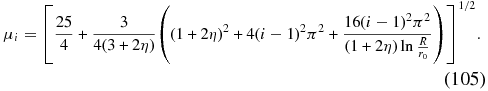
Because of the pressure balance condition, intrinsically relating the momentum and spatial diffusion coefficients with the rate of adiabatic cooling, the most sensitive parameters determining the solution are (1) the Mach number of the solar wind MA = V0/Vc, where Vc denotes the speed of the solar wind compressional waves, (2) the location of the inner and outer spatial boundaries r0 and R, and (3) the location and extent of the adopted outer ring spatial source distribution. By studying in detail four different spatial boundary conditions (reflecting and/or free-escape at the inner and outer boundaries r0 and R), we demonstrated that only for the case of a reflecting inner and a free-escape outer boundary does one small eigenvalue λ1 < (15M2A/4)[1 − 0.4M−2A]2 exist, yielding a flattest power-law index μ1 = 5, so that the power-law distribution f∝p−5 results at sufficiently large momentum values. The other three spatial boundary conditions imply steeper momentum spectra.
We illustrated our results for the favorite reflecting inner and free-escape outer boundary by adopting a uniform outer ring spatial source distribution (between 0.5R and 0.9R) and a Mach number of MA = 1.35. The calculated momentum spectra inside and outside this source distribution indeed show the flattening toward the p−5-spectrum at high momenta. The radial profiles of STPs first slightly decrease because of the reflecting boundary condition at r = 0.1R before they increase significantly at r ⩾ 0.4R. By comparing with observed radial gradients of STPs it should be possible to determine the free parameters of our solution.
Our explanation for the f∝p−5 power-law momentum spectrum of STPs is based on the pressure balance concept, implying that the timescale of effective turbulent momentum diffusion of particles is kept in balance with the timescale of adiabatic cooling in the expanding solar wind. This is reasonable in the supersonic part of the solar wind, where adiabatic deceleration dominates all other loss mechanisms. However, f∝p−5 momentum spectra are also frequently observed in the heliosheath where adiabatic cooling is negligible. In the heliosheath, particle losses due to charge exchange and particle escape from active acceleration regions are major loss mechanisms that can also limit the development of the power-law slope (see Zhang & Schlickeiser 2012 for details). It is the balance between stochastic acceleration and (any) loss mechanisms that may result in a near p−5-momentum spectrum.
The work of T.A. and R.S. was partially supported by the Deutsche Forschungsgemeinschaft through grants Schl 201/23-1 and Schl 201/25-1. M.Z. acknowledges partial support by NASA grants NNX08AP91G, NNX09AG29G, and NNX09AB24G.
APPENDIX: LARGE EIGENVALUES λi ⩾ (η + (1/2))2
In this case we set

A.1. Cases A and D
For the free-escape boundary conditions at R in these two cases, we obtain

A.1.1. Case A
Free-escape at the inner boundary r0 in this case then requires

implying

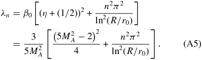
Likewise, Equation (A3) provides for the eigenvalues according to Equations (A1) and (63)
It remains to determine the expansion coefficients cn in Equation (A4) from the initial condition (59), i.e.,
With solution (A4) used in Equation (66) we obtain
Applying the orthonormality condition (65) to the initial condition then yields for arbitrary but specified special source distributions the expansion coefficients
A.1.2. Case D
Instead of Equation (74) we find here the solution

implying
The inner reflecting boundary  then yields the transcendental equation
which has an infinite number of solutions. For (η + (1/2))ln (R/r0) ≫ 1 the solutions are given by

A.2. Cases B and C
Instead of Equation (89) we obtain here
A.2.1. Case B
The inner reflecting boundary condition  is then fulfilled by the eigenvalues

providing the same eigenvalue equation (A5) as in case A. Here the eigensolutions read
The expansion coefficients cn are given by using the eigensolutions (A15) in Equation (A8).
A.2.2. Case C
Instead of Equation (91) we obtain here

so that the inner free-escape boundary condition M(r0) = 0 yields the transcendental equation
which has an infinite number of solutions for ν. For ln (R/r0) ≫ 2/(1 + 2η) one finds approximately
Footnotes
- 3
As mentioned earlier, most of the solar wind magnetic turbulence (about 85% according to Bieber et al. 1996) is in the form of axisymmetric transverse 2D turbulence. We do not know how much of it appears as compressive modes. Even if the compressive turbulence is isotropically distributed, giving rise to an isotropic spatial diffusion coefficient κ(C), the projection onto the radial propagation direction yields the radial diffusion coefficient (6). For mathematical convenience we neglect the additional spatial diffusion coefficient perpendicular to the radial direction resulting from an isotropic κ(C), as we are mostly interested in the radial variations of the STPs.