


ABSTRACT
A survey toward 674 Planck cold clumps of the Early Cold Core Catalogue (ECC) in the J = 1–0 transitions of 12CO, 13CO, and C18O has been carried out using the Purple Mountain Observatory 13.7 m telescope. Six hundred seventy-three clumps were detected with 12CO and 13CO emission, and 68% of the sample has C18O emission. Additional velocity components were also identified. A close consistency of the three line peak velocities was revealed for the first time. Kinematic distances are given for all the velocity components, and half of the clumps are located within 0.5 and 1.5 kpc. Excitation temperatures range from 4 to 27 K, slightly larger than those of Td. Line width analysis shows that the majority of ECC clumps are low-mass clumps. Column densities  span from 1020 to 4.5 × 1022 cm−2 with an average value of (4.4 ± 3.6) × 1021 cm−2.
  cumulative fraction distribution deviates from the lognormal distribution, which is attributed to optical depth. The average abundance ratio of the 13CO to C18O in these clumps is 7.0 ± 3.8, higher than the terrestrial value. Dust and gas are well coupled in 95% of the clumps. Blue profile asymmetry, red profile asymmetry, and total line asymmetry were found in less than 10% of the clumps, generally indicating that star formation is not yet developed. Ten clumps were mapped. Twelve velocity components and 22 cores were obtained. Their morphologies include extended diffuse, dense, isolated, cometary, and filament, of which the last is the majority. Twenty cores are starless, and only seven cores seem to be in a gravitationally bound state. Planck cold clumps are the most quiescent among the samples of weak red IRAS, infrared dark clouds, UC H ii candidates, extended green objects, and methanol maser sources, suggesting that Planck cold clumps have expanded the horizon of cold astronomy.
Export citation and abstract BibTeX RIS
1. INTRODUCTION
Large samples significantly improve our understanding of star formation. At the beginning of star formation studies in the early 1970s, the Palomar Sky Survey (PSS) plates provided astronomers with optical-selected nebulae as targets of star-forming regions. The cataloged Sharpless H ii regions (Sharpless 1959) from PSS served as sources for investigating gas and dust properties of molecular cloud complexes (Evans et al. 1977; Harvey et al. 1977). Nearby dark cores as well as cloud fragments were from Lynds dark nebula (Strom et al. 1975; Snell et al. 1980; Clark & Johnson 1981). With visual inspection, 70 small opaque sports were chosen for the surveys of low-mass cores with 13CO, C18O, and NH3, respectively (Myers et al. 1983; Myers & Benson 1983). A number of sources resulting from these earliest observations are still primary examples of low-mass star formation. However, the "optical dark" selection method is limited for probing star forming in deep molecular clouds. Bally & Lada (1983) chose infrared sources for detecting high velocity outflows in high-mass star formation regions. Particularly, IRAS point sources afforded plenty of samples for high-mass star formation regions. Based on the similar shapes of the far-infrared flux distribution of all embedded O-type stars, the IRAS color–color criteria were used to choose UC H ii region candidates (Wood & Churchwell 1989) and further refined by molecular line studies (Cesaroni et al. 1992; Watson et al. 1997). Precursors of UC H ii regions were also obtained from luminous IRAS sources and used for a number of surveys to examine the early characteristics of high-mass star formation (Molinari et al. 1996; Sridharan et al. 2002; Beuther et al. 2002; Wu et al. 2006). In recent years, earlier samples for high-mass star formation come from infrared dark clouds (IRDCs) surveyed by the Midcourse Space Experiment (MSX). These are extinction features against the bright mid-infrared background of the Galaxy (Egan et al. 1998). A number of starless massive cores were detected, which have narrower line widths and lower rotation temperatures than both UC H ii region precursors and UC H ii regions but have similar masses (Rathborne et al. 2006; Sridharan et al. 2005). However, MSX is limited to |b| ⩽ 6° of our Galaxy.
Now Planck surveys provide a wealth of early sources that are cold and have an unprecedented complete space distribution. The cold core Catalogue of Planck Objects (C3PO) includes 10,783 sources that are mainly cold clumps, intermediate structures of the fragmentation scenario. Their temperatures and densities range from 7 to 17 K and 30 to 105 cm−3, respectively, derived from the fluxes in the three highest frequency Planck bands (353, 545, 857 GHz) and the 3000 GHz of the IRAS band (Planck Collaboration et al. 2011a). This enables us to probe the characteristics of the prestellar phase or starless clumps. The all-sky nature of the Planck cold clump sample is particularly useful for studying the global properties of Galactic star formation. A follow-up study with high-resolution observations by Herschel revealed extended regions of cold dust with color temperatures down to 11 K. The results show different evolutionary stages ranging from a quiescent, cold filament to clumps with star-formation activities (Juvela et al. 2010).
These known properties of Planck cold clumps currently were revealed with various bands of continuum emissions and only a set of eight C3PO sources selected from a different environment (Planck Collaboration et al. 2011b) were investigated with molecular lines. Examination with molecular lines is another essential aspect for understanding the properties of the Planck cold clumps. Molecular line studies of the Planck clumps, which are an unbiased sample of cold dust clumps in the Milky Way, will provide clues for probing a number of critical questions about clumps and star formation. What are the morphologies, physical parameters, and their variations in the Galaxy? What are the initial conditions of star formation, which we do not yet know? What are the dynamic factors in a variety of the clumps and is there any premonition of collapse? Is there any depletion and what are cold chemistry phenomena? In which environment can the cold clumps exist? What is the highest Galactic latitude where stars can form? CO is the most common tool for probing molecular regions. Although there is "dark gas" which is undetected in the available CO and H i surveys (Planck Collaboration et al. 2011c), CO is still a basic probe with which to address the above questions.
In this paper we report a survey of Planck cold clumps with J = 1–0 lines of 12CO and its major isotopes, 13CO and C18O, using the telescope of the Purple Mountain Observatory (PMO) at Qinghai province in western China. Our target sources are chosen from the Early Cold Core Catalogue (ECC), which are the most reliable detections of C3PO clumps. Thus far we have surveyed 674 sources with single-point observations and mapped a subset of 10 clumps in different locations. In Section 2 the observations are described. In Section 3 we present the results. The discussions are given in Section 4 and a summary is given in Section 5.
2. OBSERVATIONS
Using the 13.7 m telescope of Qinghai Station of the PMO at De Ling Ha, the survey toward the ECC clumps with 12CO (1–0) and 13CO (1–0) lines was carried out from 2011 January to May. The half-power beam width at the 115 GHz frequency band is 56''. The pointing and tracking accuracies are better than 5''. The main beam efficiency is ∼50%. A newly installed SIS superconducting receiver with nine beam arrays was employed as the front end. The 12CO (1–0) line was observed at the upper sideband and the other two lines were observed simultaneously at the lower sideband. The typical system temperature (Tsys) in single sideband mode is around 110 K and varies by about 10% for each beam. A fast Fourier transform spectrometer was used as the back end, with a total bandwidth of 1 GHz and 16,384 channels. The equivalent velocity resolution is 0.16 km s−1 for the 12CO (1–0) line and 0.17 km s−1 for the 13CO (1–0) and C18O (1–0) lines, respectively. The position switch mode was adopted for single point observations. The off position for each "off" source was carefully chosen from an area within 3° of the "on" source, which has no or extremely weak CO emission based on the CO survey of the Milky Way (Dame et al. 1987, 2001). For those regions without CO data, we chose the off positions based on the IRAS 100 μm images. The integration time at the on/off position is 30 s.
We also mapped 10 sources that have rather strong CO emission. The On-The-Fly (OTF) observing mode was applied for mapping observations. The antenna continuously scanned a region of 22' × 22' centered on the Planck cold clumps with a scan speed of 20'' s−1. The rms noise level was 0.2 K in the main beam antenna temperature T*A for 12CO (1–0), and 0.1 K for 13CO (1–0) and C18O (1–0). Since the edges of the OTF maps are rather noisy, only the central 14' × 14' regions are analyzed. The OTF data were then converted to three-dimensional (3D) cube data with a grid spacing of 30''. The IRAM software package GILDAS was used for the data reduction (Guilloteau & Lucas 2000).
3. RESULTS
To make the observation with a sufficiently high elevation for the 13.7 m telescope at De Ling Ha, our samples were chosen from the ECC with a decl. ⩾ −20°. There are 674 sources from the ECC that satisfy this criterion. The names and coordinates of the 674 clumps are listed in Table 1 (Columns 1–7). One clump marked with "**" is without detection, and needs further checking. There are 36 clumps without suitable background reference positions for the CO emission observations, which are marked with "*" after their names and are excluded from further analysis. Clumps with latitude higher than 25° are referred to as high latitude clumps. There are 41 high latitude clumps. According to Dame et al. (1987), the distributions of the detected clumps are assigned to different molecular complexes. The regions and corresponding longitude and latitude scopes are shown in Columns 1–3 of Table 2. The fourth column of Table 2 gives a number of clumps in each complex. Six hundred seventy-three clumps were detected to have the 12CO and 13CO emission, and 68% of the clumps have the C18O emission. One hundred and eight additional velocity components were identified in both the 12CO and 13CO emission, 50% of which have C18O emission. We made a Gaussian function fitting for each distinguishable velocity component of the spectral lines. The results of emissions and their physical parameters are presented in the following.
Table 1. Surveyed ECC Clump Catalogue
| Name | Glon | Glat | R.A.(J2000) | Decl.(J2000) | R.A.(B1950) | Decl.(B1950) | Region |
|---|---|---|---|---|---|---|---|
| (°) | (°) | (h m s) | (d m s) | (h m s) | (d m s) | ||
| G001.38+20.94 | 1.3842772 | 20.941952 | 16 34 38.06 | −15 46 40.71 | 16 31 46.85 | −15 40 30.16 | Ophiuchus |
| G001.84+16.58 | 1.845703 | 16.587652 | 16 50 12.91 | −18 04 22.37 | 16 47 18.48 | −17 59 15.82 | Ophiuchus |
| G003.73+16.39 | 3.7353513 | 16.393143 | 16 55 21.78 | −16 43 35.31 | 16 52 28.86 | −16 38 50.32 | Ophiuchus |
| G003.73+18.30 | 3.7353513 | 18.308161 | 16 48 54.69 | −15 36 02.09 | 16 46 03.29 | −15 30 50.23 | Ophiuchus |
| G004.02+16.64 | 4.0209961 | 16.646044 | 16 55 10.45 | −16 21 23.27 | 16 52 17.98 | −16 16 37.51 | |
| G004.19+18.09 | 4.1967773 | 18.092196 | 16 50 42.47 | −15 22 25.13 | 16 47 51.29 | −15 17 20.75 | |
| G004.15+35.77 | 4.152832 | 35.777241 | 15 53 29.82 | −04 38 52.39 | 15 50 51.56 | −04 30 01.93 | High Glat |
| G004.17+36.67 | 4.1748047 | 36.678967 | 15 50 42.66 | −04 04 20.84 | 15 48 05.00 | −03 55 20.10 | High Glat |
| G004.41+15.90 | 4.4165034 | 15.907708 | 16 58 35.99 | −16 28 36.07 | 16 55 43.28 | −16 24 04.69 | |
| G004.46+16.64 | 4.4604487 | 16.646044 | 16 56 11.73 | −16 00 51.08 | 16 53 19.65 | −15 56 09.62 | |
| G004.54+36.74 | 4.5483394 | 36.748764 | 15 51 14.27 | −03 47 40.14 | 15 48 36.88 | −03 38 41.35 | High Glat |
| G004.81+37.02 | 4.8120112 | 37.028599 | 15 50 52.79 | −03 27 20.38 | 15 48 15.74 | −03 18 20.28 | High Glat |
| G004.92+17.95 | 4.9218745 | 17.954901 | 16 52 50.41 | −14 53 40.51 | 16 49 59.75 | −14 48 45.05 | |
| G005.03+19.07 | 5.0317378 | 19.076056 | 16 49 19.74 | −14 09 20.80 | 16 46 30.04 | −14 04 10.73 | |
| G005.29+11.07 | 5.2954097 | 11.072874 | 17 17 19.97 | −18 30 57.71 | 17 14 24.31 | −18 27 45.91 | |
| G005.29+14.47 | 5.2954097 | 14.477516 | 17 05 31.09 | −16 36 07.96 | 17 02 38.08 | −16 32 05.81 | |
| G005.31+10.78 | 5.3173823 | 10.78794 | 17 18 23.02 | −18 39 22.30 | 17 15 27.16 | −18 36 15.00 | |
| G005.69+36.84* | 5.6909175 | 36.84193 | 15 53 11.88 | −03 00 56.50 | 15 50 35.24 | −02 52 04.98 | High Glat |
| G005.80+19.92 | 5.8007808 | 19.926863 | 16 48 13.56 | −13 04 14.26 | 16 45 25.16 | −12 58 59.65 | |
| G006.08+20.26 | 6.0864253 | 20.264484 | 16 47 44.35 | −12 39 21.78 | 16 44 56.44 | −12 34 05.17 | |
| G006.04+36.74* | 6.04248 | 36.748764 | 15 54 10.81 | −02 50 56.32 | 15 51 34.33 | −02 42 08.46 | High Glat |
| G006.32+20.44 | 6.3281245 | 20.443523 | 16 47 40.85 | −12 22 03.36 | 16 44 53.28 | −12 16 46.52 | |
| G006.41+20.56 | 6.4160151 | 20.562996 | 16 47 28.67 | −12 13 52.53 | 16 44 41.26 | −12 08 34.85 | |
| G006.70+20.66 | 6.7016597 | 20.66263 | 16 47 46.71 | −11 57 20.05 | 16 44 59.61 | −11 52 03.63 | |
| G006.96+00.89 | 6.965332 | 0.895288 | 17 57 59.28 | −22 29 20.42 | 17 54 57.90 | −22 29 05.02 | Fourth quad |
| G006.94+05.84 | 6.9433589 | 5.8479061 | 17 39 41.49 | −19 58 05.07 | 17 36 43.62 | −19 56 29.92 | Fourth quad |
| G006.98+20.72 | 6.9873042 | 20.722441 | 16 48 12.55 | −11 42 10.17 | 16 45 25.73 | −11 36 55.55 | |
| G007.14+05.94 | 7.1411128 | 5.9416566 | 17 39 47.47 | −19 45 05.14 | 17 36 49.87 | −19 43 30.43 | Fourth quad |
| G007.53+21.10 | 7.5366206 | 21.101799 | 16 48 08.77 | −11 03 53.56 | 16 45 22.69 | −10 58 38.70 | |
| G007.80+21.10 | 7.8002925 | 21.101799 | 16 48 43.20 | −10 51 47.54 | 16 45 57.35 | −10 46 35.08 |
Only a portion of this table is shown here to demonstrate its form and content. A machine-readable version of the full table is available.
Download table as: DataTypeset image
Table 2. Molecular Complexes Associated with the Cold Clumps
| Region | l | b | Number | T12 | T13 | T18 | FWHM(12) | FWHM(13) | FWHM(18) |  |
Tex | τ(13) | X13/X18 | σNT | σTherm | σ3D |
|---|---|---|---|---|---|---|---|---|---|---|---|---|---|---|---|---|
| [°,°] | [°,°] | (K) | (K) | (K) | (km s−1) | (km s−1) | (km s−1) | (1021 cm−2) | (K) | (km s−1) | (km s−1) | (km s−1) | ||||
| First quad | [12,100] | [−10,10] | 84 | 2.69(1.20) | 1.85(0.77) | 0.96(0.72) | 2.70(2.23) | 1.73(1.34) | 0.96(0.72) | 5.7(5.1) | 9.4(2.4) | 1.1(0.9) | 5.6(3.3) | 0.75(0.60) | 0.17(0.02) | 1.34(1.02) |
| Second quad | [98,180] | [−4,10] | 70 | 2.57(1.23) | 1.67(0.77) | 0.85(0.51) | 2.09(1.18) | 1.42(0.68) | 0.85(0.51) | 4.5(3.4) | 9.5(2.1) | 0.9(0.5) | 7.6(3.3) | 0.62(0.29) | 0.17(0.02) | 1.13(0.49) |
| Third quad | [180,279] | [−4,10] | 43 | 2.57(1.11) | 1.51(0.64) | 1.05(0.40) | 2.90(1.00) | 1.74(0.67) | 1.05(0.40) | 4.7(2.6) | 9.1(2.0) | 0.7(0.3) | 7.0(2.9) | 0.73(0.28) | 0.17(0.02) | 1.31(0.47) |
| Fourth quad and ctr | [300,15] | [−8,8] | 6 | 3.09(0.44) | 1.54(0.59) | 2.81(5.01) | 3.03(2.57) | 1.83(1.96) | 2.81(5.01) | 4.2(2.6) | 9.5(0.9) | 0.8(0.4) | 4.4(2.3) | 0.77(0.83) | 0.17(0.01) | 1.39(1.42) |
| Anticenter | [175,210] | [−9,7] | 16 | 2.95(0.85) | 1.90(0.77) | 0.80(0.44) | 2.63(1.09) | 1.47(0.61) | 0.80(0.44) | 4.7(2.1) | 9.3(1.7) | 0.9(0.3) | 7.6(1.1) | 0.67(0.24) | 0.17(0.02) | 1.20(0.39) |
| Aquila South | [27,40] | [−21,−10] | 2 | 4.69(0.65) | 2.78(0.63) | 0.34(0.03) | 0.83(0.16) | 0.58(0.09) | 0.34(0.03) | 3.1(0.4) | 12.8(1.3) | 0.9(0.1) | 9.0(0.2) | 0.24(0.04) | 0.20(0.01) | 0.54(0.05) |
| Cephens | [99,143] | [8,22] | 87 | 2.60(0.93) | 1.66(0.64) | 0.69(0.29) | 1.94(0.87) | 1.13(0.43) | 0.69(0.29) | 3.5(1.9) | 8.8(1.8) | 1.0(0.5) | 5.4(2.1) | 0.48(0.18) | 0.16(0.02) | 0.88(0.30) |
| High Glat | |b| ⩾25 | 41 | 3.30(1.12) | 1.84(0.97) | 0.46(0.18) | 1.47(0.66) | 0.89(0.40) | 0.46(0.18) | 3.0(2.0) | 10.5(2.0) | 0.8(0.5) | 11.6(5.5) | 0.37(0.17) | 0.18(0.02) | 0.72(0.26) | |
| Oph-Sgr | [8,40] | [9,24] | 9 | 3.23(1.49) | 2.11(1.08) | 0.42(0.16) | 1.30(0.46) | 0.81(0.29) | 0.42(0.16) | 3.0(1.6) | 10.2(2.7) | 0.9(0.5) | 6.1(2.9) | 0.34(0.13) | 0.18(0.02) | 0.67(0.20) |
| Ophiuchus | [344,4] | [7,25] | 6 | 5.84(0.56) | 3.89(0.40) | 0.42(0.11) | 1.10(0.23) | 0.70(0.16) | 0.42(0.11) | 5.9(2.0) | 15.0(1.2) | 1.1(0.1) | 7.0(5.6) | 0.29(0.07) | 0.21(0.01) | 0.63(0.10) |
| Orion | [180,225] | [−25,5] | 82 | 3.58(1.90) | 2.19(1.01) | 0.76(0.35) | 2.12(1.02) | 1.29(0.53) | 0.76(0.35) | 5.8(5.3) | 11.1(4.0) | 1.0(0.6) | 8.1(5.1) | 0.55(0.23) | 0.18(0.03) | 1.02(0.38) |
| Taurus | [152,180] | [−25,−3] | 153 | 3.15(1.32) | 2.08(0.86) | 0.62(0.26) | 1.67(0.78) | 1.07(0.42) | 0.62(0.26) | 4.2(2.9) | 10.3(2.6) | 1.0(0.7) | 6.2(3.4) | 0.45(0.18) | 0.18(0.02) | 0.85(0.29) |
| Other | 75 | 3.45(1.61) | 1.97(1.22) | 0.52(0.21) | 1.51(0.68) | 0.92(0.45) | 0.52(0.21) | 3.4(2.4) | 10.5(3.3) | 0.9(0.7) | 7.4(4.4) | 0.38(0.20) | 0.18(0.03) | 0.75(0.31) |
Download table as: ASCIITypeset image
3.1. Emission Components and Characteristics of Line Profiles
Most of the observed clumps have a single velocity component in CO emission. Among the 673 sources, 123 have double velocity components and 16 have possible double velocity components; 18 have three velocity components and 10 have possible triple velocity components. Multiple components or blend emission were detected in 52 cold sources. The spectral line of each distinguishable component was fitted with a Gaussian function. Centroid velocity Vlsr, antenna temperature T*A, and FWHM  were obtained for all three CO lines, which are given in Table 3. Centroid velocity of 13CO was taken as the systemic velocity of each velocity component and listed in the second column of Table 4. Dense core masses are related to molecular line widths (Wang et al. 2009). We adopted an average value of 13CO line width of 1.3 km s−1 for the nearby dark cores (Myers & Benson 1983) as a criterion to distinguish high-mass and low-mass clumps. If a clump contains one or more velocity components with a 13CO line width larger than 1.3 km s−1, it is considered to be a candidate of high-mass clumps (group H), otherwise, it is taken as a candidate for low-mass clumps (group L). In some of the observed clumps, the spectral lines of the emission components depart from a Gaussian profile, which probably reflects the state of gas or originates from systematic motions and star formation activities. We classify the different non-Gaussian profiles with the following characters: BA+: blue profile; RA+: red profile; BA: blue asymmetric; RA: red asymmetric; De: possible depletion; BW: blue wing; RW: red wing; W: wings; P: pedestal; Dob: double components; T: three components; and M.B: multiple or blended components.
Table 3. Observed Line Parameters
| Name | Vlsr(12) | FWHM(12) | TA(12) | Vlsr(13) | FWHM(13) | TA(13) | Vlsr(18) | FWHM(18) | TA(18) | |
|---|---|---|---|---|---|---|---|---|---|---|
| (km s−1) | (km s−1) | (K) | (km s−1) | (km s−1) | (K) | (km s−1) | (km s−1) | (K) | ||
| G001.38+20.94 | 0.61(0.01) | 1.16(0.02) | 5.67(0.18) | 0.74(0.01) | 0.78(0.01) | 3.98(0.09) | 0.74(0.01) | 0.54(0.03) | 1.26(0.09) | |
| G001.84+16.58 | 6.05(0.01) | 1.32(0.03) | 5.58(0.17) | 5.87(0.01) | 0.69(0.01) | 4(0.09) | 5.87(0.01) | 0.38(0.02) | 1.67(0.09) | |
| G003.73+16.39 | 6.44(0.01) | 1.11(0.02) | 5.56(0.17) | 6.17(0.01) | 0.71(0.01) | 3.41(0.09) | 6.17(0.02) | 0.53(0.07) | 0.77(0.09) | RA |
| G003.73+18.30 | 4.44(0.01) | 1.36(0.02) | 6.68(0.21) | 4.37(0.01) | 0.97(0.01) | 4.34(0.08) | 4.32(0.01) | 0.43(0.02) | 2.45(0.08) | |
| G004.02+16.64 | 5.92(0.01) | 0.69(0.02) | 5.5(0.18) | 5.87(0) | 0.49(0.01) | 3.81(0.09) | 5.86(0.02) | 0.34(0.05) | 0.71(0.08) | |
| G004.19+18.09 | 3.64(0.01) | 1.63(0.02) | 5.94(0.19) | 3.5(0.01) | 1.23(0.01) | 4.12(0.09) | 3.73(0.02) | 0.44(0.05) | 0.94(0.08) | Dob |
| G004.19+18.09 | 6.68(0.01) | 0.88(0.02) | 6.63(0.19) | 6.69(0.01) | 0.62(0.01) | 3.16(0.09) | ||||
| G004.15+35.77 | 2.47(0.01) | 1.92(0.03) | 4.72(0.14) | 2.61(0.01) | 1.06(0.02) | 3.17(0.09) | ||||
| G004.17+36.67 | 2.55(0.01) | 0.93(0.02) | 5.08(0.17) | 2.47(0.01) | 0.71(0.01) | 3.27(0.08) | ||||
| G004.41+15.90 | 4.78(0.01) | 0.57(0.01) | 6.11(0.15) | 4.73(0) | 0.48(0.01) | 3.69(0.09) | ||||
| G004.46+16.64 | 5.16(0.01) | 1.66(0.02) | 6.1(0.15) | 5.34(0.01) | 1.19(0.02) | 3.67(0.09) | 5.55(0.01) | 0.43(0.03) | 1.42(0.09) | BA+ |
| G004.54+36.74 | 2.46(0.01) | 1.17(0.02) | 4.5(0.17) | 2.53(0.01) | 0.76(0.02) | 2.94(0.09) | 2.54(0.04) | 0.44(0.1) | 0.44(0.09) | |
| G004.81+37.02 | 3.6(0.01) | 1.51(0.02) | 4.47(0.13) | 3.71(0.01) | 1.04(0.02) | 2.91(0.09) | 3.82(0.04) | 0.66(0.09) | 0.46(0.08) | |
| G004.92+17.95 | 3.54(0.02) | 1.49(0.03) | 3.77(0.18) | 3.72(0.01) | 0.63(0.03) | 3.26(0.17) | 3.71(0.01) | 0.32(0.03) | 0.98(0.08) | |
| G005.03+19.07 | 3.83(0.01) | 1.25(0.02) | 7.17(0.19) | 3.77(0.01) | 0.99(0.01) | 3.86(0.09) | 3.81(0.03) | 0.65(0.07) | 0.73(0.09) | |
| G005.29+11.07 | 4.37(0.01) | 0.92(0.01) | 7.55(0.18) | 4.22(0) | 0.63(0.01) | 4.07(0.09) | 4.14(0.01) | 0.34(0.04) | 1.16(0.09) | |
| G005.29+14.47 | 3.76(0.01) | 0.4(0.01) | 5.07(0.18) | 3.74(0.01) | 0.3(0.02) | 1.21(0.09) | ||||
| G005.31+10.78 | 4.53(0.01) | 1.24(0.02) | 6.56(0.19) | 4.38(0.01) | 0.88(0.01) | 4.1(0.1) | ||||
| G005.69+36.84 | 0.56(0.03) | 1.39(0.06) | 3.84(0.17) | 0.6(0.03) | 0.96(0.07) | 0.81(0.09) | Dob | |||
| G005.69+36.84 | 2.25(0.04) | 1.62(0.08) | 3.4(0.17) | 2.33(0.01) | 0.9(0.02) | 3.01(0.09) | 2.27(0.01) | 0.4(0.02) | 1.46(0.09) | |
| G005.80+19.92 | 3.45(0.01) | 1.41(0.02) | 6.11(0.18) | 3.06(0.01) | 0.89(0.01) | 3.87(0.09) | 2.96(0.02) | 0.47(0.05) | 0.99(0.09) | |
| G006.08+20.26 | 4.03(0.01) | 1.95(0.02) | 5.23(0.16) | 3.96(0.01) | 0.91(0.01) | 4.19(0.08) | 3.97(0.01) | 0.56(0.03) | 1.16(0.08) | BA+ |
| G006.04+36.74 | 2.34(0.02) | 1.99(0.04) | 3.61(0.17) | 2.61(0.01) | 0.94(0.02) | 2.73(0.1) | 2.53(0.01) | 0.47(0.03) | 1.47(0.09) | |
| G006.32+20.44 | 4.48(0.01) | 1.6(0.02) | 4.98(0.16) | 4.32(0.01) | 0.72(0.01) | 4.25(0.09) | 4.27(0.01) | 0.38(0.02) | 1.88(0.09) | |
| G006.41+20.56 | 4.54(0.01) | 1.38(0.02) | 5.9(0.16) | 4.39(0.01) | 0.95(0.01) | 4.43(0.08) | 4.44(0.02) | 0.67(0.04) | 1.37(0.09) | |
| G006.70+20.66 | 3.49(0.01) | 2(0.03) | 4.44(0.15) | 3.76(0.01) | 1.06(0.01) | 3.97(0.08) | 3.79(0.01) | 0.66(0.04) | 1.35(0.09) | |
| G006.96+00.89 | 9.78(0.05) | 4.1(0.12) | 2.66(0.23) | 9.33(0.05) | 2.17(0.15) | 0.88(0.1) | Dob | |||
| G006.96+00.89 | 41.34(0.06) | 9.42(0.15) | 3.11(0.23) | 41.53(0.1) | 6.89(0.24) | 0.77(0.1) | 41.67(0.63) | 13.03(2.05) | 0.17(0.1) | |
| G006.94+05.84 | 5.22(0.02) | 1.57(0.04) | 3.26(0.19) | 4.86(0.02) | 0.63(0.06) | 1.21(0.1) | Dob | |||
| G006.94+05.84 | 10.59(0.02) | 2.57(0.05) | 3.38(0.19) | 10.08(0.02) | 1.39(0.03) | 2.22(0.1) | 10.05(0.03) | 0.83(0.07) | 0.77(0.09) |
Only a portion of this table is shown here to demonstrate its form and content. A machine-readable version of the full table is available.
Download table as: DataTypeset image
Table 4. Derived Parameters of Surveyed ECC Clumps
| Name | Vlsr | R | D | Z | Tex | τ(13) | N(13) | τ(18) | N(18) |  |
Ratio(12/13) | X13/X18 | σNT | σTherm | σ3D |
|---|---|---|---|---|---|---|---|---|---|---|---|---|---|---|---|
| (km s−1) | (kpc) | (kpc) | (kpc) | (K) | (1015 cm−2) | (1015 cm−2) | (1021 cm−2) | (km s−1) | (km s−1) | (km s−1) | |||||
| G001.38+20.94 | 0.74 | 7.47 | 1.1 | 0.39 | 14.8 | 1.2 | 7.3 | 0.2 | 1.6 | 6.5 | 2.1 | 4.6 | 0.32 | 0.21 | 0.67 |
| G001.84+16.58 | 5.87 | 4.51 | 4.16 | 1.19 | 14.6 | 1.2 | 6.5 | 0.4 | 1.5 | 5.7 | 2.7 | 4.3 | 0.29 | 0.21 | 0.61 |
| G003.73+16.39 | 6.17 | 5.87 | 2.75 | 0.78 | 14.6 | 0.9 | 5.7 | 0.1 | 1.0 | 5.0 | 2.5 | 5.9 | 0.29 | 0.21 | 0.63 |
| G003.73+18.30 | 4.32 | 6.48 | 2.14 | 0.67 | 16.8 | 1.0 | 10.6 | 0.5 | 2.7 | 9.4 | 2.2 | 4.0 | 0.41 | 0.23 | 0.80 |
| G004.02+16.64 | 5.86 | 6.10 | 2.52 | 0.72 | 14.4 | 1.2 | 4.3 | 0.1 | 0.6 | 3.9 | 2.0 | 7.7 | 0.20 | 0.21 | 0.50 |
| G004.19+18.09 | 3.73 | 6.88 | 1.71 | 0.53 | 15.3 | 1.2 | 12.1 | 0.2 | 1.0 | 10.8 | 1.9 | 12.2 | 0.52 | 0.22 | 0.97 |
| G004.19+18.09 | 6.69 | 5.92 | 2.73 | 0.85 | 16.7 | 0.6 | 4.9 | 4.4 | 3.0 | 0.25 | 0.23 | 0.59 | |||
| G004.15+35.77 | 2.61 | 7.13 | 1.7 | 0.99 | 12.9 | 1.1 | 7.4 | 6.6 | 2.7 | 0.45 | 0.20 | 0.85 | |||
| G004.17+36.67 | 2.47 | 7.19 | 1.64 | 0.98 | 13.6 | 1.0 | 5.2 | 4.7 | 2.0 | 0.29 | 0.20 | 0.62 | |||
| G004.41+15.90 | 4.73 | 6.62 | 1.96 | 0.54 | 15.7 | 0.9 | 4.3 | 3.8 | 2.0 | 0.19 | 0.22 | 0.50 | |||
| G004.46+16.64 | 5.55 | 6.37 | 2.23 | 0.64 | 15.6 | 0.9 | 10.6 | 0.3 | 1.5 | 9.4 | 2.3 | 7.1 | 0.50 | 0.22 | 0.95 |
| G004.54+36.74 | 2.54 | 7.25 | 1.56 | 0.93 | 12.4 | 1.0 | 4.9 | 0.1 | 0.4 | 4.3 | 2.4 | 11.5 | 0.32 | 0.19 | 0.64 |
| G004.81+37.02 | 3.82 | 6.79 | 2.15 | 1.30 | 12.3 | 1.0 | 6.6 | 0.1 | 0.7 | 5.9 | 2.2 | 9.9 | 0.44 | 0.19 | 0.83 |
| G004.92+17.95 | 3.71 | 7.10 | 1.48 | 0.46 | 10.9 | 2.0 | 4.3 | 0.3 | 0.7 | 3.8 | 2.7 | 6.5 | 0.26 | 0.18 | 0.55 |
| G005.03+19.07 | 3.81 | 7.08 | 1.5 | 0.49 | 17.8 | 0.8 | 9.9 | 0.1 | 1.2 | 8.8 | 2.3 | 8.0 | 0.41 | 0.23 | 0.82 |
| G005.29+11.07 | 4.14 | 7.09 | 1.44 | 0.28 | 18.6 | 0.8 | 6.8 | 0.2 | 1.1 | 6.1 | 2.7 | 6.5 | 0.26 | 0.24 | 0.61 |
| G005.29+14.47 | 3.74 | 7.20 | 1.35 | 0.34 | 13.6 | 0.3 | 0.8 | 0.7 | 5.6 | 0.11 | 0.20 | 0.40 | |||
| G005.31+10.78 | 4.38 | 7.03 | 1.51 | 0.28 | 16.6 | 1.0 | 9.0 | 8.0 | 2.3 | 0.37 | 0.22 | 0.75 | |||
| G005.69+36.84 | 0.6 | 8.33 | 0.21 | 0.13 | 11.1 | 0.2 | 1.6 | 1.4 | 6.9 | 0.40 | 0.18 | 0.77 | |||
| G005.69+36.84 | 2.27 | 7.60 | 1.13 | 0.68 | 10.2 | 2.1 | 5.5 | 0.6 | 1.2 | 4.9 | 2.0 | 4.6 | 0.38 | 0.18 | 0.72 |
| G005.80+19.92 | 2.96 | 7.52 | 1.05 | 0.36 | 15.7 | 1.0 | 8.3 | 0.2 | 1.1 | 7.4 | 2.5 | 7.4 | 0.37 | 0.22 | 0.75 |
| G006.08+20.26 | 3.97 | 7.26 | 1.33 | 0.46 | 13.9 | 1.6 | 8.7 | 0.2 | 1.5 | 7.7 | 2.7 | 5.9 | 0.38 | 0.21 | 0.75 |
Only a portion of this table is shown here to demonstrate its form and content. A machine-readable version of the full table is available.
Download table as: DataTypeset image
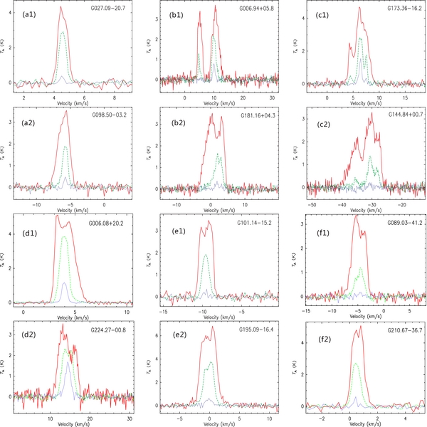
The normalized velocity difference δV = (Vthick − Vthin)/δVthin is applied to identify the blue and red profiles (Mardones et al. 1997), where Vthick is the peak velocity of 12CO (1–0), Vthin and δVthin are the systemic velocity and the optical thin line width, respectively, of optically thin lines. We use 13CO (1–0) and C18O (1–0) as the optically thin lines. If δV < −0.25, the line is classified as a "blue profile," and if δV > 0.25, the line is classified as a "red profile." The sources with blue or red profiles are listed in Table 5. We define δV(12) = (Vthick − V12)/δVthin to investigate line blue or red asymmetries where δV12 < −0.25 or >0.25, where V12 is the center velocity of 12CO (1–0). The sources with asymmetric profiles are listed in Table 6. The spectrum characteristics are denoted in the last column of Table 3. Figure 1 presents the examples of the spectra of the J = 1–0 lines of the 12CO, 13CO, and C18O with red, green, and blue colors, respectively, including single, double, and triple components and the characteristics of the spectral profiles.
Download figure:
Standard image High-resolution image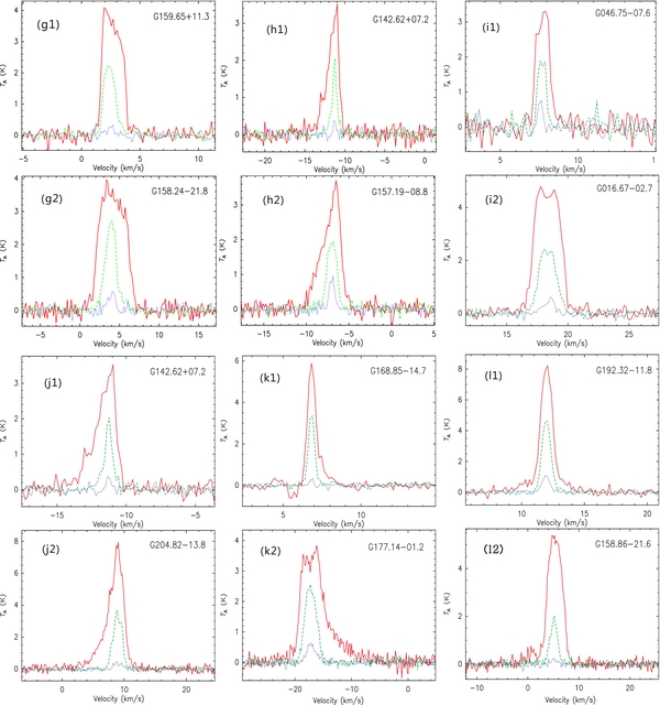
Figure 1. Examples of J = 1–0 lines of 12CO, 13CO, and C18O spectra with different profiles. The classes are as follows: (a), (b), and (c) denote single, double, and triple velocity component spectra, respectively. (d) and (e) denote blue and red profiles; "1" and "2" denote low- and high-mass groups, respectively. (f1) and (f2) denote blue and red profiles of high-latitude clumps. (g), (h), and (i) denote blue asymmetry, red asymmetry, and the center dip, respectively; (j), (k), and (l) denote blue wings, red wings, and a pedestal, respectively; "1" and "2" denote the same as above.
Download figure:
Standard image High-resolution imageTable 5. Sources with Blue or Red Line Profiles
| Name | V13 | FWHM13 | V18 | FWHM18 | V12_peak | δV_13a | δV_18b | T12_B/T12_R | ΔTc | Profile | Region |
|---|---|---|---|---|---|---|---|---|---|---|---|
| (km s−1) | (km s−1) | (km s−1) | (km s−1) | (km s−1) | |||||||
| G004.46+16.64 | 5.34(0.01) | 1.19(0.02) | 5.55(0.01) | 0.43(0.03) | 4.95 | −0.33 | −1.40 | 1.42 | 1.88 | Blue profile | Others |
| G006.08+20.26 | 3.96(0.01) | 0.91(0.01) | 3.97(0.01) | 0.56(0.03) | 3.25 | −0.78 | −1.29 | 1.09 | 0.42 | Blue profile | Others |
| G089.03−41.28 | −4.63(0.03) | 1.93(0.06) | −5.37 | −0.38 | 0.63 | 1.23 | 0.63 | Blue profile | High Glat | ||
| G097.09+10.12 | −2.71(0.03) | 1.09(0.05) | −2.67(0.04) | 0.63(0.09) | −3.33 | −0.57 | −1.05 | 1.57 | 1.01 | Blue profile | Others |
| G111.33+19.94 | −7.21(0.01) | 0.83(0.03) | −7.24(0.02) | 0.58(0.05) | −8.13 | −1.11 | −1.53 | 1.21 | 0.5 | Blue profile | Cephens |
| G111.77+13.78 | −3.81(0.01) | 0.85(0.03) | −3.68(0.05) | 0.46(0.15) | −4.29 | −0.56 | −1.33 | 2.18 | 1.69 | Blue profile | Cephens |
| G111.77+20.26 | −8.06(0.01) | 1.15(0.03) | −8.09(0.04) | 0.88(0.11) | −8.62 | −0.49 | −0.60 | 1.84 | 1.55 | Blue profile | Cephens |
| G111.97+20.52 | −7.92(0.02) | 0.9 (0.05) | −7.91(0.03) | 0.48(0.08) | −8.62 | −0.78 | −1.48 | 1.69 | 0.86 | Blue profile | Cephens |
| G117.11+12.42 | 3.87(0.01) | 0.96(0.03) | 3.92(0.02) | 0.53(0.06) | 3.32 | −0.57 | −1.13 | 1.25 | 0.78 | Blue profile | Cephens |
| G126.49−01.30 | −11.94(0.02) | 1.9 (0.04) | −11.74(0.04) | 0.91(0.09) | −13 | −0.56 | −1.38 | 1.19 | 0.6 | Blue profile | Second quad |
| G130.14+13.78 | −1.53(0.02) | 1.46(0.06) | −1.43(0.05) | 0.69(0.14) | −2.55 | −0.70 | −1.62 | 1.11 | 0.23 | Blue profile | Cephens |
| G155.45−14.59 | 1.97(0.02) | 1.39(0.05) | 2.13(0.03) | 0.61(0.1) | 0.83 | −0.82 | −2.13 | 2.50 | 1.93 | Blue profile | Taurus |
| G158.37−20.72 | 7.13(0.01) | 2.35(0.02) | 7.05(0.03) | 1.4(0.08) | 6.03 | −0.47 | −0.73 | 1.11 | 0.80 | Blue profile | Taurus |
| G164.94−08.57 | −0.7(0.01) | 1.71(0.03) | −0.63(0.05) | 1.31(0.11) | −1.66 | −0.56 | −0.79 | 1.73 | 1.89 | Blue profile | Taurus |
| G181.84+00.31 | 3.3(0.02) | 1.49(0.04) | 3.49(0.05) | 0.81(0.12) | 2.21 | −0.73 | −1.58 | 1.29 | 0.74 | Blue profile | Third quad |
| G190.17−13.78 | 1.14(0.01) | 1.39(0.02) | 0.74 | −0.29 | 1.12 | 0.54 | Blue profile | Orion | |||
| G210.01−20.16 | 8.1(0.02) | 1.83(0.04) | 8.33(0.09) | 0.68(0.22) | 7.27 | −0.45 | −1.56 | 1.25 | 0.99 | Blue profile | Orion |
| G224.27−00.82 | 14.39(0.02) | 3.04(0.04) | 14.45(0.02) | 1.61(0.05) | 13.09 | −0.43 | −0.84 | 1.28 | 0.7 | Blue profile | Third Quad |
| G093.22−04.59 | 3.87(0.01) | 1.51(0.03) | 3.9(0.06) | 1.14(0.15) | 4.41 | 0.36 | 0.45 | 1.1 | 0.29 | Red profile | First quad |
| G101.14−15.28 | −9.58(0.01) | 0.98(0.03) | −9.18 | 0.41 | 0.29 | 0.92 | 0.29 | Red profile | Others | ||
| G121.92−01.71 | −14.07(0.01) | 1.39(0.03) | −14.12(0.08) | 1.11(0.16) | −13.46 | 0.44 | 0.59 | 0.87 | 0.5 | Red profile | Second quad |
| G145.81+10.97 | −14.94(0.02) | 1.06(0.04) | −14.31 | 0.59 | 0.29 | 0.90 | 0.29 | Red profile | Others | ||
| G157.10−08.70 | −7.48(0.02) | 1.43(0.04) | −7.48(0.03) | 0.9(0.08) | −6.98 | 0.35 | −1.40 | 0.55 | 1.8 | Red profile | Taurus |
| G169.84−07.61 | 6.46(0.01) | 0.67(0.02) | 6.39(0.01) | 0.31(0.03) | 6.83 | 0.55 | 1.42 | 0.90 | 0.35 | Red profile | Taurus |
| G172.85+02.27 | −17.22(0.02) | 3.18(0.06) | −17.49(0.07) | 1.47(0.17) | −15.83 | 0.44 | 1.13 | 0.90 | 0.45 | Red profile | Second quad |
| G182.15−17.95 | 9.4(0.01) | 0.86(0.02) | 9.35(0.03) | 0.53(0.06) | 10.11 | 0.83 | −0.64 | 0.71 | 1.26 | Red profile | Orion |
| G182.54−25.34 | 1.06(0.05) | 1.45(0.1) | 1.78 | 0.50 | 0.87 | 0.74 | 0.87 | Red profile | High Glat | ||
| G188.04−03.71 | 3.12(0.03) | 1.39(0.06) | 3.15(0.08) | 0.9(0.16) | 4.03 | 0.65 | −1.02 | 0.73 | 0.52 | Red profile | Third quad |
| G192.28−11.33 | 10.19(0.01) | 1.47(0.01) | 10.13(0.04) | 0.84(0.11 | 10.81 | 0.42 | 0.81 | 0.75 | 1.61 | Red profile | Orion |
| G195.09−16.41 | −0.08(0.01) | 1.84(0.02) | −0.1(0.05) | 1.3(0.13) | 0.47 | 0.30 | −0.47 | 0.89 | 0.77 | Red profile | Orion |
| G210.67−36.77 | 0.47(0.01) | 0.6(0.02) | 0.45(0.06) | 0.24(0.09) | 0.81 | 0.57 | 1.50 | 0.84 | 0.93 | Red profile | High Glat |
| G216.69−13.88 | 8.72(0.02) | 1.88(0.06) | 8.81(0.07) | 0.8(0.13) | 9.71 | 0.53 | 1.13 | 0.91 | 0.32 | Red profile | Orion |
| G219.35−09.70 | 12.5(0.02) | 1.65(0.04) | 12.45(0.03) | 0.93(0.07) | 13.41 | 0.55 | 1.03 | 0.67 | 0.76 | Red profile | Orion |
Notes. aδV_13 = (V12_peak-V13)/FWHM13. bδV_18 = (V12_peak-V18)/FWHM18. cΔT = abs(T12_b-T12_r).
Download table as: ASCIITypeset image
Table 6. Sources with Blue or Red Line Asymmetry
| Name | FWHM13 | FWHM18 | V12 | V12_peak | δV(12)_13a | δV(12)_18b | Profile | Region |
|---|---|---|---|---|---|---|---|---|
| (km s−1) | (km s−1) | (km s−1) | (km s−1) | |||||
| G018.39+19.39 | 0.52(0.01) | 0.27(0.04) | −0.46(0.01) | −0.61 | −0.29 | −0.56 | Blue asymmetry | Oph-Sgr |
| G027.70−21.02 | 0.47(0.04) | 4.95(0.02) | 4.78 | −0.36 | Blue asymmetry | |||
| G108.10+13.19 | 1.04(0.04) | 0.43(0.03) | −4.81(0.03) | −5.17 | −0.35 | −0.84 | Blue asymmetry | Cephens |
| G111.66+20.20 | 1.34(0.03) | 0.79(0.09) | −8.17(0.03) | −8.64 | −0.35 | −0.59 | Blue asymmetry | Cephens |
| G143.85+11.49 | 1.63(0.08) | −13.78(0.06) | −14.3 | −0.32 | Blue asymmetry | Others | ||
| G147.96−08.02 | 0.63(0.1) | −28.39(0.04) | −28.59 | −0.32 | Blue asymmetry | Others | ||
| G156.90−08.49 | 1.92(0.06) | 0.53(0.05) | −7.72(0.04) | −8.56 | −0.44 | −1.58 | Blue asymmetry | Taurus |
| G158.24−21.80 | 1.63(0.03) | 1.13(0.13) | 4.09(0.02) | 3.45 | −0.39 | −0.57 | Blue asymmetry | Taurus |
| G158.40−21.86 | 1.21(0.03) | 0.92(0.1) | 4.54(0.01) | 4.13 | −0.34 | −0.45 | Blue asymmetry | Taurus |
| G159.65+11.39 | 1.11(0.02) | 0.99(0.27) | 2.61(0.01) | 1.9 | −0.64 | −0.72 | Blue asymmetry | Others |
| G171.43−17.36 | 1.16(0.02) | 0.4(0.03) | 7.47(0.02) | 6.99 | −0.41 | −1.20 | Blue asymmetry | Taurus |
| G172.92−16.74a | 0.7(0.02) | 0.51(0.08) | 5.06(0.02) | 4.9 | −0.23 | −0.31 | Blue asymmetry? | Taurus |
| G172.92−16.74b | 0.87(0.02) | 0.58(0.05) | 6.96(0.02) | 6.49 | −0.54 | −0.81 | Blue asymmetry | Taurus |
| G173.18−09.12 | 0.5(0.02) | 0.51(0.09) | 6.23(0.02) | 6.03 | −0.40 | −0.39 | Blue asymmetry | Taurus |
| G179.14−06.27 | 0.52(0.02) | 7.69(0.02) | 7.45 | −0.46 | Blue asymmetry | Anticenter | ||
| G182.02−00.16 | 1.28(0.05) | 0.89(0.18) | 3.91(0.02) | 3.43 | −0.38 | −0.54 | Blue asymmetry | Third quad |
| G190.08−13.51 | 1.62(0.03) | 1.11(0.02) | 0.64 | −0.29 | Blue asymmetry | Orion | ||
| G196.21−15.50 | 2.29(0.08) | 3.51(0.02) | 2.88 | −0.28 | Blue asymmetry | Orion | ||
| G227.70+11.18 | 0.59(0.14) | 14.98(0.02) | 14.78 | −0.34 | Blue asymmetry | Others | ||
| G003.73+16.39 | 0.71(0.01) | 0.53(0.07) | 6.44(0.01) | 6.67 | 0.32 | 0.43 | Red asymmetry | Ophiuchus |
| G118.34+08.66 | 0.72(0.05) | 0.41(0.14) | −2.07(0.03) | −1.79 | 0.39 | 0.68 | Red asymmetry | Cephens |
| G118.36+21.74 | 0.86(0.06) | −3.88(0.04) | −3.5 | 0.44 | Red asymmetry | Cephens | ||
| G142.25+05.43 | 0.97(0.03) | −10.18(0.01) | −9.85 | 0.34 | Red asymmetry | Second quad | ||
| G142.62+07.29 | 0.66(0.03) | 0.36(0.11) | −11.42(0.02) | −10.97 | 0.68 | 1.25 | Red asymmetry | Second quad |
| G157.19−08.81 | 1.29(0.03) | 0.74(0.06) | −7(0.02) | −6.49 | 0.40 | 0.69 | Red asymmetry | Taurus |
| G157.25−01.00 | 0.67(0.01) | 0.36(0.02) | 5.27(0.01) | 5.5 | 0.34 | 0.64 | Red asymmetry | Second quad |
| G157.58−08.89 | 1.07(0.04) | 0.41(0.03) | −6.07(0.03) | −5.37 | 0.65 | 1.71 | Red asymmetry | Taurus |
| G159.58−32.84 | 1.38(0.07) | 3.79(0.02) | 4.43 | 0.46 | Red asymmetry | High Glat | ||
| G174.50−19.88 | 0.81(0.02) | 0.56(0.09) | 7.7(0.01) | 7.96 | 0.32 | 0.46 | Red asymmetry | Taurus |
| G175.16−16.74 | 1.11(0.03) | 0.8(0.1) | 5.7(0.03) | 6.23 | 0.48 | 0.66 | Red asymmetry | Second quad |
| G195.00−16.95 | 1.1(0.02) | 0.51(0.04) | −1.99(0.01) | −1.76 | 0.21 | 0.45 | Red asymmetry | Orion |
| G221.46−17.89 | 0.46(0.03) | 0.17(0.66) | 7.99(0.03) | 8.12 | 0.28 | 0.76 | Red asymmetry | Orion |
Notes. aδV(12)_13 = (V12_peak-V12)/FWHM13. bδV(12)_18 = (V12_peak-V12)/FWHM18.
Download table as: ASCIITypeset image
3.2. Observed Parameters
The histograms of the line center (peak) velocity difference between the lines of 12CO and 13CO (V12–V13) and those of 13CO and C18O (V13–V18) lines are shown in Figures 2(a) and (b). The distributions (blue solid histograms) of both the V12 − V13 and V13 − V18 are quite symmetric around the zero, and are fitted with a normal distribution (red curve). However, their distributions are much narrower than a standard normal distribution (red curve), but have a sharp peak at zero (see Figures 2(a) and (b)). Ninety-four percent of the clumps have V12 − V13 less than 3σ of the velocity resolution (0.17 km s−1) given by the spectrometer, and 98% of the clumps have V13 − V18 less than 3σ of the velocity resolution. The velocity correlations between lines of 12CO–13CO and 13CO–18CO are shown in Figures 2(c) and (d). Y = (1.002 ± 0.001)X + (0.005 ± 0.016) for V12 (Y) to V13 (X) and Y = (0.992 ± 0.005)X + (0.140 ± 0.057) for V13 (Y) to V18 (X) show very good correlations and the correlation coefficient is 100%. This is the first time good agreement of the center velocities of the 12CO and its main isotopes, the 13CO and C18O lines, has been shown with such a large sample. These results show that the peak velocities of the three CO lines agree very well, and demonstrate that they originate from the same emission regions. Comparisons of Figures 2(a) and (b) with Figures 2(c) and (d) show the agreement between Vlsr of the 13CO and C18O lines is better than that of the 12CO and 13CO lines, which may suggest that the 12CO is easily affected by dynamic factors in the clump or its environment.
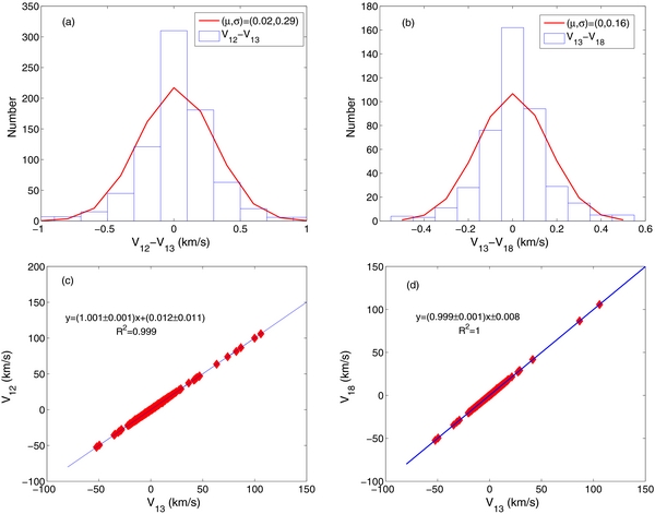
Figure 2. Line center velocities of the J = 1–0 lines of 12CO, 13CO, and C18O. (a) and (b) are the histogram and the normal distribution fits for the difference between V12 and V13, V13 and V18, respectively. The mean μ and standard deviation σ of the normal distributions are presented in the upper-right boxes; (c) and (d) plot for V12 vs. V13 and V13 vs. V18, respectively.
Download figure:
Standard image High-resolution imageSince there are fewer sources in which C18O lines were detected compared with those in which 13CO lines were detected, we adopt the center velocity of 13CO as the systemic velocity of the clumps in the following analysis. For the components without 13CO (1–0) emission, the center velocities of 12CO were adopted as the systemic velocity.
The main beam antenna temperatures of the three transitions for all the components detected were obtained. T12 ranges from 0.5 to 12 K. The three clumps G209.28−19.62 (12 K), G192.54−11.56 (9.2 K), and G207.35−19.82 (8.8 K), temperatures which are all located in the Orion region, have the highest. Generally, the antenna temperatures of 13CO and C18O are also high in the 12CO emission strong clumps. For the above three clumps, T13 and T18 are 6.8, 1.4; 5.0, 0.6; and 3.1, 0.4 K, respectively. The ratio of T12/T13 is between 2.8 and 1.8, showing that the 12CO line emissions have large opacity. The ratio of T13/T18 ranges between 4.5 and 8.3, with an average value of 6.0 which is close to the terrestrial value. However, the ratio may be different in different regions, for example, in the Ophiuchus complex, the antenna temperatures of the three transitions are 6.7, 4.4, and 2.5 K for G003.73+18.30 and 5.9, 4.4, and 1.4 K for G006.41+20.56. The ratio of T13/T18 is 1.8 and 3.1 for the two clumps, respectively, which is much less than 5.5, suggesting that the 13CO lines are optically thick. For all the detected components, the histograms of T12 and the ratios of T12/T13 and T13/T18 are present in Figures 3(a)–(c), respectively. The peak of T12 is around 3 K. For the ratio of T12/T13, the mean value is 2.2 with a standard deviation of 1.4, showing that the 12CO (1–0) line emissions of the cold clumps are generally optically thick. The mean value of the ratio of T13/T18 is 3.9 with a standard deviation of 1.7.
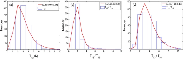
Figure 3. Frequency distributions of the antenna temperature T12, the ratio of T12/T13, and T13/T18.
Download figure:
Standard image High-resolution imageWe found that all the distributions of the observed parameters as well as the derived parameters seemed to skew to the right with a long tail at the high value side. We try to depict their distributions with a lognormal distribution. The probability density function (PDF) of a lognormal distribution is
where x is the value of the variable, the parameters μ and σ are the mean and standard deviation, respectively, of the variable's natural logarithm. The Kolmogorov-Smirnov test (K-S test) is applied to identify whether the parameters follow a lognormal distribution. The decision to reject or accept the null hypothesis is based on comparing the P-value with the desired significance level, which is 0.05 in this paper. If the P-values from the K-S test are larger than 0.05, the parameter should follow the reference distribution. The statistics and K-S test results of the parameters are summarized in Table 7.
Table 7. A Statistical Analysis of Parameters
| Stat | V12 − V13 | V13 − V18 | T12 | T12/ T13 | T13/ T18 | FWHM(12) | FWHM(13) | FWHM(18) |  |
Tex | τ(13) | X13/X18 | σNT | σTherm | σ3D | σNT/σTherm |
|---|---|---|---|---|---|---|---|---|---|---|---|---|---|---|---|---|
| (km s−1) | (km s−1) | (K) | (km s−1) | (km s−1) | (km s−1) | (1021 cm−2) | (K) | (km s−1) | (km s−1) | (km s−1) | ||||||
| Statistics | ||||||||||||||||
| Numbera | 782 | 437 | 904 | 782 | 437 | 904 | 782 | 437 | 782 | 782 | 782 | 437 | 782 | 782 | 782 | 782 |
| Mean | 0.02 | 0 | 3.08 | 2.15 | 3.88 | 2.03 | 1.27 | 0.76 | 4.4 | 10.1 | 0.93 | 7.0 | 0.53 | 0.17 | 0.98 | 3.09 |
| std | 0.29 | 0.16 | 1.37 | 1.35 | 1.71 | 1.28 | 0.77 | 0.73 | 3.6 | 2.6 | 0.56 | 3.8 | 0.31 | 0.02 | 0.51 | 1.83 |
| Normal distribution fit | Lognormal distribution fit | |||||||||||||||
| μ | 0.02 | 0 | 1.02 | 0.65 | 1.26 | 0.56 | 0.10 | −0.44 | 1.22 | 2.29 | −0.24 | 1.83 | −0.77 | −1.76 | −0.12 | 0.99 |
| σ | 0.29 | 0.16 | 0.48 | 0.43 | 0.45 | 0.55 | 0.51 | 0.53 | 0.78 | 0.24 | 0.62 | 0.46 | 0.51 | −0.12 | 0.43 | 0.53 |
| P | 0 | 0 | 0 | 0 | 0.234 | 0.636 | 0.830 | 0.515 | 0 | 0.227 | 0 | 0.388 | 0.889 | 0.227 | 0.374 | 0.822 |
Notes. aOnly the parameters of 13CO components are analyzed, but we also include those 12CO components without 13CO emission in statistics of T12 and FWHM(12). Thirty-nine clumps without suitable reference positions in observations are excluded in statistics.
Download table as: ASCIITypeset image
The distributions of T12 and T12/T13 have a similar characteristic. Both have a power-law-like long tail, but cannot be described well with a lognormal distribution. The tail of the distribution of T13/T18 is less than those of T12 and T12/T13, suggesting that T12 may be a more sensitive physical element than T13 and T18 for star formation. The distribution of T13/T18 has a lognormal shape with a P-value for the K-S test as high as 0.234.
From Table 3 one can see that the line widths of the emission components are generally narrow. Most of the clumps have line widths smaller than 1.3 km s−1. There are 162 high-mass clump candidates; among these, 68 have 2 or more velocity components. The clumps at high latitude all are low-mass clump candidates with a single component except for G159.23−34.49, which is in the high-mass group and has two components. Figure 4(a) presents the distributions of the FWHM of all three lines: the mean values and the standard deviations of the three line widths are 2.0 ± 1.3, 1.3 ± 0.8, and 0.8 ± 0.7 km s−1, respectively. The shapes of all the distributions are similar to each other and are lognormally distributed.
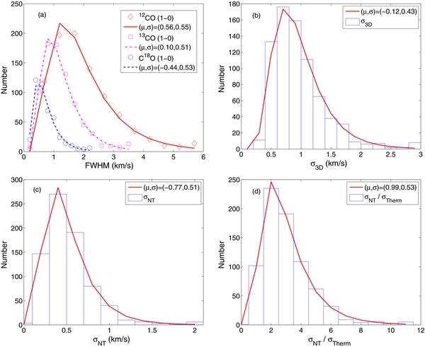
Figure 4. Frequency distributions of the line FWHMs and velocity dispersions. (a) Distributions and lognormal fitting of the FWHMs of the CO, 13CO, and C18O lines. (b) Histogram and the lognormal fitting of the 13CO line 3D velocity dispersion. (c) Velocity dispersion of nonthermal motion 13CO lines. (d) Histogram and lognormal fitting of the ratio of the 13CO line nonthermal and thermal motion. The mean μ and standard deviation σ of the lognormal distribution fits are presented in the upper-right boxes in each panel.
Download figure:
Standard image High-resolution image3.3. Derived Physical Parameters
The excitation temperature derived from the radiation transfer equation is
Here, Tr is the brightness temperature corrected with beam efficiency ηb. Assuming 12CO emission is optically thick (τ ≫ 1) and a filling factor of f = 1, the excitation temperature Tex can be straightforwardly obtained. The Tex is given in Column 6 of Table 4. We assume that the excitation temperatures of 13CO and C18O are the same as that of the 12CO (1–0) in the following analysis. The values range from 3.9 K to 27 K, wider than the dust temperature range 7–17 K (Planck Collaboration et al. 2011a). The mean value with the standard deviation is 10 ± 2.6 K, which is smaller than the mean value of the dust temperature (12.8 ± 1.6 K) based on aperture photometry with a local background subtraction by Herschel photometric observations toward 71 Planck cold fields (Juvela et al. 2012), indicating the gas may be heated by the dust. There are 12 clumps with Tex > 17 K. All of the hottest clumps are located in the Orion and Taurus regions, which suggests that high excitation temperature may be related to star formation conditions. Ninety-three components with Tex < 7 K are referred to as coldest clumps among which G093.66+04.66 (3.9 K) is in the first quadrant, and G098.10+15.83 (5.0 K) and G112.63+20.80 (5.8 K) are in Cepheus. All other coldest clumps are the weaker components of the clumps with double or three emission components. The Tex histogram and its lognormal fit are shown in Figure 5. Its distribution can be well fitted by a lognormal shape with a P-value of the K-S test as large as 0.227, but the tail of the distribution seems to be much smaller than that of line widths and velocity dispersions. In the following analysis Tex was taken as the gas kinetic temperature assuming the local thermodynamic equilibrium (LTE) holds.
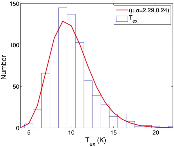
Figure 5. Histogram and the lognormal-PDF fitting of excitation temperatures.
Download figure:
Standard image High-resolution imageBoth the optical depths τ13 and τ18 at the emission peak of the corresponding lines were calculated with Equation (2) assuming the filling factor f = 1; these are listed in Columns 7 and 9 in Table 4. τ13 ranges from 0.1 to 4.1. The clumps with the largest τ13 include G026.45−08.02 (3.2) and G058.07+03.29 (3.2) of the first quadrant, G164.94−08.57 (4.1) and G179.10−06.27 (3.9) in Taurus, and G182.04+00.41 (3.8) located at anticenter. For the 10 clumps with the smallest optical depth (0.1), all of them are the minor components of the multiple-component sources except for G121.88−08.76. Figure 6(a) shows the histogram of τ13 and its lognormal fitting. The mean value is 0.93 ± 0.56.
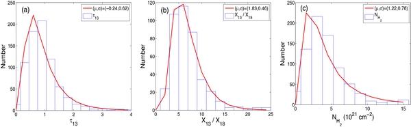
Figure 6. Histograms of τ13, ratio [X_13/X_18], and column density  , and their lognormal-PDF fitting.
Download figure:
Standard image High-resolution imageThe column density of a molecular line can be obtained with the theory of radiation transfer and molecular excitation as follows (Garden et al. 1991):
where B, μ, and J are the rotational constant, the permanent dipole moment, and the rotational quantum number of the lower state of the molecular transition. Column densities of the 13CO and C18O molecules were calculated and given in Columns 8 and 10 of Table 4. The maximum C18O column densities of the Planck clumps are 1.1 × 1016 cm−2 and 1.3 × 1015 cm−2 in G028.56−00.24 and G160.51−16.84, respectively, and the smallest ones are 1.0 × 1014 cm−2 in G26.93−20.68 and G102.72−25.96. The column densities of the C18O span a wider range than those of the nearby dark clouds (Myers et al. 1983) which are from 3 × 10¹⁴ to 2.7 × 1015 cm−2. The different column density ranges between our sample and the nearby dark clouds may be attributed to the larger space distribution of Planck cold clumps than the nearby dark clouds.
The 13CO column densities were calculated for 782 velocity components. For the 437 components with both C18O and 13CO column densities, the abundance ratio of X13/X18 was calculated and listed in Column 13 of Table 4. The histogram and the lognormal distribution of X13/X18 fitting are presented in Figure 6(b). The distribution shape of the ratio X13/X18 is similar to that of τ13. The mean value of X13/X18 is 7.0 ± 3.8, higher than that of the terrestrial ratio 5.5. The distribution of X13/X18 can be well depicted by a lognormal distribution with a P-value of the K-S test as high as 0.388.
Molecular hydrogen column densities of each velocity component were derived according to the column densities of the 13CO. The fractional abundance of [H2]/[13CO] = 89 × 104 was adopted. We also calculated the  for the components without 13CO emission by assuming 12CO (1–0) emission to be optically thin, the excitation temperature of 10 K and [H2]/[12CO] = 104, but these components are excluded in further statistics. Figure 6(c) presents the plots of the
  histogram and its lognormal fitting. It spans from 1020 to 4.5 × 1022 cm−2, which is larger than that of the eight sources on average (Planck Collaboration et al. 2011b). From Herschel follow-up observations, the peak column densities of 71 clumps range from 4 × 10²⁰ to 7.4 × 10²² (Juvela et al. 2012), which are slightly larger than the column densities obtained in this work. The four clumps with the largest 13CO column densities are G209.28−19.62, G028.56−00.24, G033.70−00.01, and G158.37−20.72. The
  of G209.28−19.62 located in the Orion complex is as high as 4.5 × 1022 cm−2. G028.56−00.24 and G033.70−00.01, with
  of 3.4 and 2.8 × 1022 cm−2, are located in the first quadrant. G158.37−20.72, with
  of 2.3 × 1022 cm−2, is in Taurus, which is 7' north of NGC 1333 (Strom et al. 1976) and has a very red young star, SSV 13 (Harvey et al. 1998). The 12CO lines of all these clumps have large line widths of 2.57–9.35 km s−1, showing turbulence support for these clumps. The column density distribution (Figure 6(c)) cannot be fitted with a unique lognormal distribution, but exhibits a power-law-like tail, similar to that identified from active star formation regions (Kainulainen et al. 2009), indicating that some Planck cold clumps are located in active star-forming regions.
The one-dimensional nonthermal (σNT) and thermal (σTherm) velocity dispersions can be estimated as follows:


where  and Tex are the one-dimensional velocity dispersion of the 13CO (1–0) and excitation temperature, respectively. k is the Boltzmann's constant,
  is the mass of 13CO, mH is the mass of atomic hydrogen, and μ = 2.72 is the mean molecular weight of the gas. Then the 3D velocity dispersion σ3D can be estimated as

The 3D and nonthermal velocity dispersions shown in Figures 4(b) and (c) also present a similar distribution as line widths. As shown in Table 7, the P-values of the K-S test for a lognormal hypothesis for line widths and velocity dispersions are all much larger than 0.05, indicating that their distributions can be remarkably well described by a lognormal fit. The lognormal behaviors of volume or column density in molecular clouds were frequently reported in recent observations (Ridge et al. 2006; Froebrich et al. 2007; Goodman et al. 2009), which are often interpreted as a consequence of supersonic turbulence in the observed clouds (Vázquez-Semadeni 1994). From our results, the effect of supersonic turbulence in the clouds should be more likely reflected in the lognormal behaviors of the distributions of line widths and velocity dispersions than in the distributions of column density. Figure 4(d) plots the distribution for the ratios of σNT to σTherm. One can see that most of the clumps have σNT larger than σTherm, indicating that turbulent motions dominate in these clouds. The shape of their ratio distribution is similar to the distributions of the FWHM of the three transitions, the σ3D and σNT, but the tail part is narrower than the others, which may suggest that the thermal motions may not be as sensitive as nonthermal motions for revealing star formation activity.
3.4. Mapping Results
In the 10 mapped clumps, 12 velocity components were detected. Six of them have FWHMs of 13CO (1–0) larger than 1.3 km s−1 and the other four belong to group L. The CO line profiles of the clump G089.64−06.59, one of the velocity components of G157.60−12.17, G179.29+04.20, and G196.21−15.50, show a blue asymmetric signature. The integrated intensities are shown in the contour maps in Figure 7. The morphologies of these clumps are different. G001.38+20.94 and G180.92+04.53 show both diffuse features and a dense clump. G108.85−00.80, G157.60−12.17b, and G196.21−15.50 exhibit a filamentary shape with a chain of dense clumps. G161.43−35.59 and G194.80−03.41 also appear as a dumbbell in filamentary structure. Four cores are detected in G006.96+00.89a and G161.43−35.59, respectively. G049.06−04.18 is an isolate clump while G089.64−06.59 shows a cometary-like structure. Filamentary structures are the majority among these clumps, which is consistent with the Herschel follow-up observation results (Juvela et al. 2012). Juvela et al. (2012) also found that the filaments often fragment into substructures. Such behavior is revealed in the gas emission too as in G006.96+00.89a shown in Figure 7.
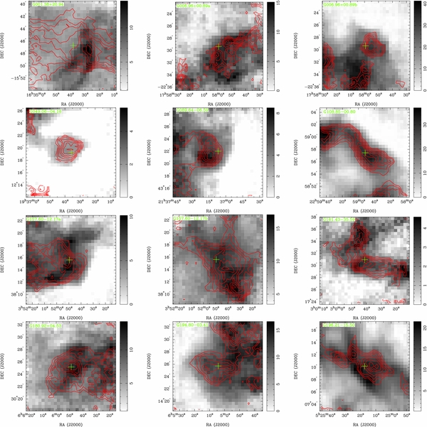
Figure 7. Integration intensity images of the mapped clumps: contours for the 13CO line and the gray scale for the 12CO lines. The contours are from 30% to 90% in a step of 10% of the peak value.
Download figure:
Standard image High-resolution imageThere are 22 cores identified with two-dimensional Gaussian fits to the 10 mapped sources. The physical parameters of these cores are presented in Table 8. The positions of the cores are shown as offset relative to the reference positions in Column 4. Deconvolved sizes a and b (Column 5) are the major and minor angular sizes of the cores and measured from the contours at half of the maximum intensity of the 13CO (1–0) lines. The radius R = ((ab)1/2/2)D, where D is the distance, in Column 6 distributes from several tenths to about 3 of kpc. Columns 7–12 list the clump parameters: Tex,  , velocity dispersions, and volume density
  /2R, respectively. Then the core mass can be derived as
  , where
  is the mass of a hydrogen molecule and μg = 1.36 is the mean atomic weight of the gas. Core mass calculated with LTE assumption is given in Column 13. Columns 14 and 15 are the virial mass and the Jeans mass, respectively (see the next section). The final three columns are the morphology, the group, and the location of the clumps. The column density of the cores ranges from 1.3 to 7.7 × 1021 cm−2. The LTE masses of the cores range from 9 to 1.5 × 10⁴ M☉ with a median value of 110 M☉. In the Herschel follow-up observations, the 26 identified filaments have column densities ranging from 0.9 to 19.2 × 1021 cm−2 and masses ranging from 3.2 × 10³ with a median value of 120 M☉ (Juvela et al. 2012), which are consistent with the case of the cores in this work.
Table 8. Parameters of the 10 Mapped Clumps
| Name | Vlsr | d | Offset | Deconvolved Size | R | Tex |  |
σTherm | σNT | σ3D | n | MLTE | Mvir | MJ | Group | Region |
|---|---|---|---|---|---|---|---|---|---|---|---|---|---|---|---|---|
| (km s−1) | (kpc) | ('', '') | ('' × ''(°)) | (pc) | (K) | (1021 cm−2) | (km s−1) | (km s−1) | (km s−1) | (103 cm−3) | (M☉) | (M☉) | (M☉) | |||
| G001.38+20.94 | 0.74 | 1.1 | (−110,−41) | 677 × 428(67.9) | 1.4 | 14.1(0.9) | 5.3(1.7) | 0.21(0.01) | 0.33(0.09) | 0.67(0.13) | 0.6 | 751 | 150 | 43 | L | Ophiuchus |
| G006.96+00.89a_1 | 9.33 | 2.21 | (5,−91) | 187 × 119(−8.1) | 0.8 | 9.9(0.4) | 3.2(0.7) | 0.17(0.00) | 0.88(0.19) | 1.56(0.32) | 0.6 | 141 | 453 | 496 | H | Fourth quad |
| G006.96+00.89a_2 | 9.33 | 2.21 | (−90,30) | 149 × 102(−42.5) | 0.7 | 9.7(0.5) | 2.6(0.9) | 0.17(0.00) | 0.70(0.20) | 1.25(0.34) | 0.6 | 78 | 240 | 260 | Fourth quad | |
| G006.96+00.89a_3 | 9.33 | 2.21 | (−207,39) | 301 × 64(−70.9) | 0.7 | 9.4(0.3) | 3.2(1.0) | 0.17(0.00) | 0.92(0.01) | 1.61(0.17) | 0.7 | 122 | 449 | 544 | Fourth quad | |
| G006.96+00.89a_4 | 9.33 | 2.21 | (−334,66) | 268 × 143(89.1) | 1.0 | 8.9(0.7) | 2.7(0.7) | 0.16(0.01) | 1.02(0.30) | 1.79(0.51) | 0.4 | 204 | 783 | 945 | Fourth quad | |
| G006.96+00.89b | 41.67 | 5.36 | (−64,−1) | 203 × 161(38.2) | 2.3 | 10.7(1.1) | 6.8(2.6) | 0.18(0.01) | 1.52(0.22) | 2.66(0.37) | 0.5 | 2579 | 3873 | 2905 | H | Fourth quad |
| G049.06−04.18 | 9.93 | 0.6 | (16,41) | 239 × 194(−51.9) | 0.3 | 8.9(1.2) | 1.3(0.5) | 0.16(0.01) | 0.15(0.04) | 0.39(0.05) | 0.7 | 9 | 11 | 7 | L | First quad |
| G089.64−06.59 | 12.51 | 0.6 | (81,−20) | 320 × 187(−0.9) | 0.4 | 10.2(0.9) | 3.4(1.5) | 0.18(0.01) | 0.40(0.09) | 0.74(0.15) | 1.5 | 30 | 45 | 38 | L | First quad |
| G108.85−00.80 | −49.51 | 5.4 | (−20,−12) | 776 × 213(45.1) | 5.3 | 11.5(3.7) | 7.7(5.4) | 0.18(0.03) | 0.89(0.28) | 1.58(0.46) | 0.2 | 14993 | 3096 | 858 | H | Second quad |
| G157.60−12.17a | −7.75 | 1.17 | (−38,−44) | 432 × 283(16.4) | 1.0 | 10.4(0.9) | 3.6(1.2) | 0.18(0.01) | 0.40(0.01) | 0.76(0.12) | 0.6 | 243 | 133 | 61 | L | Taurus |
| G157.60−12.17b_1 | −2.58 | 0.47 | (−83,−63) | 535 × 421(41.7) | 0.5 | 14.7(1.6) | 4.1(1.5) | 0.21(0.01) | 0.43(0.11) | 0.83(0.17) | 1.2 | 82 | 87 | 55 | L | Taurus |
| G157.60−12.17b_2 | −2.58 | 0.47 | (−197,−278) | 301 × 196(52.2) | 0.3 | 14.6(1.3) | 4.1(1.4) | 0.21(0.01) | 0.60(0.13) | 1.11(0.21) | 2.4 | 22 | 79 | 92 | Taurus | |
| G161.43−35.59_1 | −5.83 | 1.49 | (60,212) | 269 × 143(−12.5) | 0.7 | 9.8(0.4) | 2.3(0.5) | 0.17(0.00) | 0.29(0.06) | 0.59(0.09) | 0.5 | 79 | 57 | 29 | L | High Glat |
| G161.43−35.59_2 | −5.83 | 1.49 | (−3,−49) | 261 × 150(82) | 0.7 | 12.0(1.2) | 2.6(0.8) | 0.19(0.01) | 0.18(0.03) | 0.46(0.04) | 0.6 | 91 | 35 | 13 | High Glat | |
| G161.43−35.59_3 | −5.83 | 1.49 | (−166,−71) | 387 × 168(87.6) | 0.9 | 10.5(0.9) | 2.2(0.5) | 0.18(0.01) | 0.20(0.03) | 0.47(0.04) | 0.4 | 128 | 47 | 17 | High Glat | |
| G161.43−35.59_4 | −5.83 | 1.49 | (−303,−86) | 141 × 140(−21.1) | 0.5 | 10.7(0.9) | 1.9(0.6) | 0.18(0.01) | 0.25(0.06) | 0.53(0.09) | 0.6 | 34 | 33 | 21 | High Glat | |
| G180.92+04.53 | 0.98 | 3.62 | (0,−12) | 359 × 339(62.2) | 3.1 | 9.1(0.6) | 3.4(1.1) | 0.17(0.01) | 0.59(0.11) | 1.07(0.19) | 0.2 | 2191 | 817 | 303 | H | Third quad |
| G194.80−03.41_1 | 12.84 | 2.89 | (−4,−19) | 690 × 341(81.3) | 3.4 | 9.8(0.5) | 4.5(1.7) | 0.18(0.01) | 0.86(0.31) | 1.52(0.52) | 0.2 | 3573 | 1829 | 812 | H | Third quad |
| G194.80−03.41_2 | 12.84 | 2.89 | (−132,331) | 355 × 242(61.3) | 2.1 | 10.3(0.9) | 5.3(2.4) | 0.17(0.01) | 0.78(0.20) | 1.28(0.34) | 0.4 | 1536 | 784 | 436 | Third quad | |
| G196.21−15.50_1 | 3.76 | 0.8 | (−79,5) | 276 × 203(54.2) | 0.5 | 14.5(0.8) | 3.1(0.9) | 0.21(0.01) | 0.32(0.12) | 0.68(0.16) | 1.1 | 45 | 49 | 30 | H | Orion |
| G196.21−15.50_2 | 3.76 | 0.8 | (104,126) | 228 × 84(3.5) | 0.3 | 15.1(0.8) | 2.8(0.7) | 0.21(0.01) | 0.31(0.07) | 0.65(0.11) | 1.7 | 14 | 26 | 22 | Orion | |
| G196.21−15.50_3 | 3.76 | 0.8 | (265,85) | 256 × 89(60.8) | 0.3 | 14.6(0.6) | 2.5(0.9) | 0.21(0.00) | 0.30(0.12) | 0.66(0.15) | 1.4 | 15 | 30 | 23 | Orion |
Download table as: ASCIITypeset image
4. DISCUSSION
4.1. Line Center Velocities
The coincidence of three transitions observed toward the Planck clumps is not usual in star formation regions. Line center velocities of different molecular species could be significantly offset from the systematic velocity in active star-forming regions. In the six NH3 clumps of G084.81−01.09, the deviations between the 12CO and 13CO are all larger than 1 km s−1 (Zhang et al. 2011). Vlsr of the 12CO deviated from that of 13CO or C18O are also seen in IRDCs. In 61 IRDCs, there are 10% of sources with Vlsr deviation of ≳ 1 km s−1 from the 12CO and the C18O lines (Du & Yang 2008). The rather large discrepancy between the Vlsr of 12CO and 13CO can also be seen in the submillimeter clumps (Qin et al. 2008). The line center velocity difference of various molecular species may originate from molecular layers with different temperatures or trace different kinematical gas layers (Bergin et al. 1997; Muller et al. 2011). The deviation between V13 and V18 of the Planck clumps also tends to be smaller than those of Myers et al. (1983). All of these suggest that the cold clumps are the quietest molecular regions found so far as a whole.
4.2. Distances of the Clumps
Distance is essential for investigating the spatial distribution and physical conditions of the clumps. The Planck Collaboration et al. (2011d) have estimated the distance for 2619 C3PO clumps using various extinction signatures. They also found that there are 127 Planck cold clumps associated with IRDCs which have a kinematic distance from Simon et al. (2006). In our sample there are only two clumps close to the sources of Simon et al. (2006) at the zero latitude Galactic layer. There is certainly a part of the ECC clumps with distance estimated using extinction methods. We estimated the kinematic distances of the clumps using the Vlsr of the clumps which could be a comparison for those with known distance. We adopt the rotation curve of Clemens (1985) R☉ = 8.5 kpc and Θ☉ = 220 km s−1 in our calculation. To see the possible physical relation of the components in clumps with double and triple peaks, the distance of each component was calculated. For the clumps within the inside of the solar circle there are two solutions. The clumps are perhaps located at the front of the Galactic bulk of the diffuse background, since extinction is rising along a line of sight that crosses a dust clump (Planck Collaboration et al. 2011a). For this reason, the near value of the distances was adopted. Among our sample there are a number of clumps that are located in molecular complexes with known distances. Since these complexes have rather large areas and clumps residing inside them have different Vlsr, the kinematic distances of the clumps within one complex are quite different as well. Therefore, for every clump within the same complex, their distances are also given as the kinematic distances. However, in a case where there is some ambiguity about the distance of the clump, the one close to the known distance of the complex was adopted.
The histogram of the kinematic distances is plotted in Figure 8. Distances were obtained for 741 13CO components. Of the components, 51% have distances within 0.5 and 1.5 kpc. The mean value is 1.57 kpc, lower than those associated with IRDCs by Simon et al. (2006). The reason for this may be due to cloud properties; most of our clumps or components belong to the low-mass group and the IRDCs of Simon et al. (2006) are at the fourth quadrant of the mid-plane and with distances between 0.4 and 7.8 kpc (Simon et al. 2006).
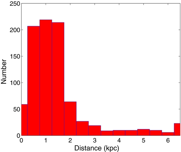
Figure 8. Frequency distribution of the kinematic distances.
Download figure:
Standard image High-resolution image4.3. Physical Parameter Distributions in the Galaxy
4.3.1. Excitation Temperature and the Ratio of Line Strengths of 12CO and 13CO
Figure 9 presents the distribution of the Tex and the ratio of T12/T13. Figures 9(a) and (c) are for radial changes and (b) and (d) are for the altitude from the Galactic plane. The excitation temperature is higher than 10 K from 4 to 8 kpc. Early observations also showed the high excitation of the gas emission at the 3–7 kpc molecular ring (Scoville & Sanders 1987). Around 8 kpc, Tex is also larger than 10 K, which may be related to the emission of the giant molecular clouds near the Sagittarius arm. The ratio of T12 to T13 is high at R ∼ 5 kpc, then deceases with R and has a valley between 5 and 8 kpc, then a lowest value at ∼6 kpc, suggesting that the brightness temperature of 13CO (1–0) is relatively high in this region.
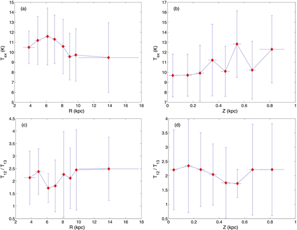
Figure 9. Variations of bin-averaged Tex and T12/T13 with distance from the Galactic center R and the altitude from the Galactic disk plane Z. The bin size in R is 1 kpc for those clumps with R < 10 pc and the clumps with R > 10 pc are put into a single bin. The bin size in Z is 0.1 pc. The clumps with Z > 1 kpc are rare and are not included in the analysis.
Download figure:
Standard image High-resolution imageFigure 9(b) shows that excitation temperature changes with the altitude. There are two peaks 11 and 13 K at Z ∼ 350 pc and ∼470 pc, respectively. The changes of the ratio of T12/T13 shown in Figure 9(d) are rather smooth and reach a low value at Z ∼ 470 pc, suggesting the brightness temperature of 13CO is relatively high at this altitude.
4.3.2. Velocity Dispersion
Variations of the velocity dispersion with the distance from the Galactic center and the altitude from the Galactic plane are investigated. The radial variations of σ3D, σNT, and the ratio of σNT/σTherm are plotted in Figures 10(a), (c), and (e), respectively. The variation of the σ3D and σNT as well as the ratio of σNT/σTherm with R are about the same and they reached the maximum at R ∼ 5 kpc, which suggests that the dynamic process is most violent at the 5 kpc Galactic ring. From 6 kpc, the σ3D, σNT, and the ratio of σNT/σTherm seem to linearly increase with R, indicating that turbulence becomes more violent in the outer part of the Galaxy.
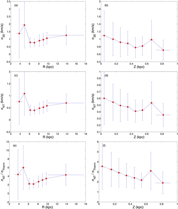
Figure 10. Variations of bin-averaged σ3D, σNT, and the ratio of σNT/σTherm of 13CO lines with R and Z. The bin sizes are the same as for Figure 9.
Download figure:
Standard image High-resolution imageFigures 10(b), (d), and (f) present changes of the velocity dispersions σ3D, σNT, and the ratio of σNT/σTherm with the altitude. One can see that they all decrease with increasing altitude from the Galactic disk to heights of 475–525 pc, showing that the turbulent process is stronger closer to the Galactic plane. At Z ∼ 680 pc all of them reached a minor peak. We found the clumps at this minor peak are distributed around (l ∼ 174°, b ∼ 17°) or (l ∼ 4°, b ∼ −17°); this minor peak may be concerned with the emission regions of Taurus and ρ Oph. From panels (e) and (f), one can see that nonthermal motion dominates the line broadening. This is the first time evidence for nonthermal line broadening has been obtained from a survey of the 13CO (1–0) lines.
One can see that there are some differences among the radial variations of the velocity dispersion and excitation temperature. The maximum of Tex–R variation is at rather high values around 4–8 kpc and reaches maximum at 6 kpc. The Tex variation is milder than that of σNT suggesting that the gas heating and cooling occur in a wider spatial region than the turbulence.
4.3.3. 13CO Opacity, X13/X18, and H2 Column Density
Figure 11(a) shows the radial variation of the optical depth of the 13CO (1–0) lines. The smallest value is at the 5 kpc ring. Between 5.5 and 8 kpc there is a high feature, then it decreases until 14 kpc. One reason for the low valley is that Tex is rather high around 5 kpc (see Figure 9(a)). Besides, its emission is relatively low compared with that of 12CO. For example, G017.22−01.47 at R = 4.90 kpc is τ13 = 0.3, Tex = 10.1 K, and T13 = 0.88 K; G033.70−00.01, R = 5.05 kpc, τ13 = 0.5, Tex = 9.2 K, and T13 = 1.12 K; and G028.56−00.24, R = 4.96 kpc, τ13 = 0.3, Tex = 10.1 K, and T13 = 0.92 K.
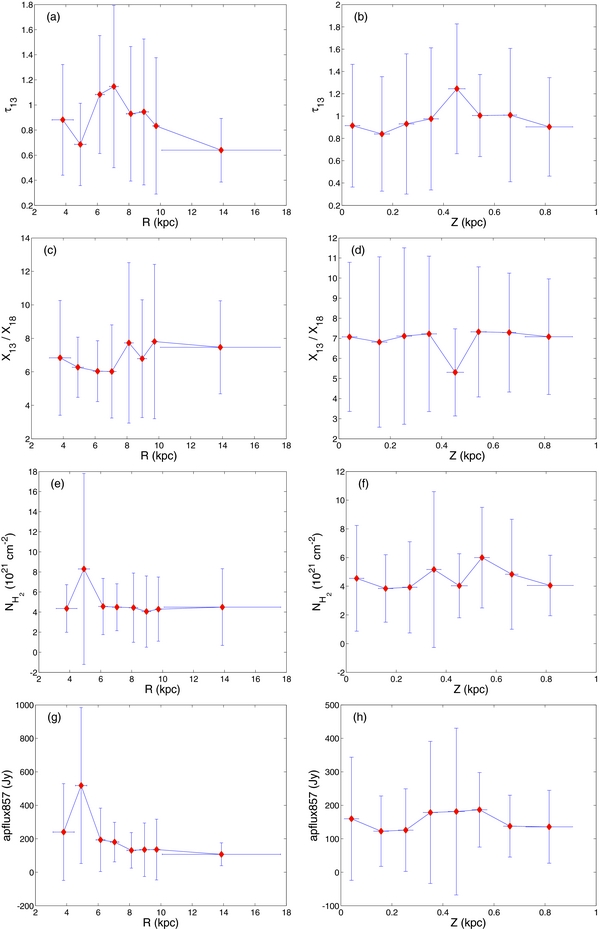
Figure 11. Variations of bin-averaged τ13, [X13]/[X18],  , and the flux at 857 GHz with R and Z.
Download figure:
Standard image High-resolution imageThe ratio of X13 to X18 presented in Figure 11(c) is rather low, between 5 and 7 kpc, and its corresponding values range from ∼6 to 7, still higher than the terrestrial value. At 8 kpc and >10 kpc the value is near 8.
Figure 11(e) shows the radial variation of the column density of hydrogen molecules. Clearly, it presents an enhancement at 5 kpc where the densest and most massive star formation regions within our Galaxy are located. Then it is almost at a similar level until it reaches the outer region except at 9 kpc where there is a minor low valley. Owing to the small τ13 around 5 kpc (see Figure 11(a)) the column density is mainly affected by the velocity dispersion σ3D or σNT shown in Figure 10. To confirm the Galactic distribution of the column density, the radial distribution of the flux density at 857 GHz dust emission detected by Planck was plotted in Figure 11(g). The variations agree with that of the column density very well. At 9 kpc the 857 GHz flux is a little higher, showing another dense structure (Scoville & Sanders 1987).
The variation of τ13 with altitude is shown in Figure 11(b). It exhibits a high feature between 350 and 550 pc and reaches its maximum at 450 pc. The change of the ratio of X13/X18 seen in Figure 11(d) seems to be opposite to that of τ13 with its lowest point at Z = 450 pc. Figure 11(f) presents the variation of the molecular hydrogen column density with Z. At Z = 300 and 500 pc, the values are higher than in the other regions. There is a low valley at Z = 450. Combining the altitude variation of τ13 and the velocity dispersion of Figures 10(b), (d), and (f) where σNT is at low values, again shows that nonthermal line width is the major factor in determining the gas column density. Between 350 and 550 pc the flux at 857 GHz is higher too, which is consistent with the variation of  as a whole. These results revealed that the column density reaches the maximum at R = 5 kpc, a low valley at Z = 450 pc, and is mainly caused by nonthermal velocity dispersion, which also has not been reported before.
4.3.4. Parameters of the Clumps in Different Molecular Complexes
For the 12 complexes included in our sample, a statistical analysis of the physical parameters was made. The corresponding average values are presented in Table 2. They display different trends. The famous star formation regions including Ophiuchus, Orion, Oph-Sgr, and Taurus harbor 250 observed clumps. They have the highest excitation temperatures and column densities. The average 13CO FWHM of these clumps is less than 1.3 km s−1. Even in Orion it is only 1.29 km s−1, suggesting that low-mass clumps are the dominant sources in the Planck cold clumps. Their nonthermal velocity dispersion is almost two times the thermal velocity except in Ophiuchus where σthermal ∼ σNT. Cephens harbors 87 observed clumps. The FWHM of the 13CO J = 1–0 line is between Orion and the above-mentioned star formation regions. σNT is also the dominant factor for the line broadening. A common characteristic can be seen in that all four quadrants and the anticenter regions have FWHMs of the 13CO J = 1–0 line ≳ 1.5 km s−1. All of them belong to the high-mass group. The σNT is about four times the σthermal, indicating that these regions have stronger dynamic processes than other star formation regions.
4.4. Line Profiles
There are 16 clumps having an absorption dip at the line center, which is rather symmetric relative to the Vlsr. Nine of them show a dip in all three transitions. They may be the candidates for the 12CO depletion. In the other seven clumps, only the 12CO line has the center dips that may originate from self-absorption. Mapping is needed to further examine the properties of the line center dips. Eighteen cores with blue profiles and fifteen cores with red profiles were identified (see Table 5). Blue profiles are a kind of typical feature of molecular clump collapse (Zhou et al. 1993) whereas the red profile could originate from the expansion of the clump or outflow motion. The ratios of the clump with the blue and red profiles to the total clump numbers of clumps are small—2.7% and 2.2%, respectively. The blue excess E = (Nb − Nr)/Nt is 0.004; here Nb, Nr, and Nt are the clump numbers with the detected blue and red profiles and the surveyed sample (Mardones et al. 1997). E of the Class -I, 0, and I clumps is 0.31, 0.30, and 0.30 shown in the HCN (3–2) line, respectively (Evans 2003), while it is 0.15–0.17 for UC H ii region precursors and 0.58 for UC H ii regions detected with HCO+(1–0) lines (Wu et al. 2007; Fuller et al. 2005). Nevertheless, in a sample of 27 Orion starless clumps, 9 have blue profiles and 10 have red ones, implying that the blue excess E is −0.04 (Velusamy et al. 2008). The ratios of the blue and red profiles to these cores are 33% and 37%, greatly exceeding those of our sample, suggesting that star formation activities occur more frequently in the Orion cores than in the Planck cold clumps. The small ratio of the blue and red profiles means that most of the Planck cold clumps do not yet have systematic star-forming motion. We also identified 19 and 13 cores with blue and red line asymmetry, respectively. Different from blue and red profiles, line asymmetry reflects the whole gas motion of the core, which may result in interaction of the core and its environment.
High velocity wings are rare in Planck cold clumps. Among the surveyed clumps, only three were detected with blue wings, six with red ones, eight with both blue and red wings, and six with a pedestal feature, showing rather rare star formation feedback activities.
4.5. Conditions of the Clumps at High Latitudes
There are 41 clumps located at latitudes higher than 25°. Six clumps have two velocity components and one has three. Nine of the clumps belong to the high-mass group. Tex is intermediate among the 12 complexes (see Table 2). The column density is 3 × 1021 cm−2 on average. σNT tends to be smaller among the 12 complexes but still larger than those in the Ophiechs and Oph-Sgr. Core G089.03−41.28 has a blue profile while cores G182.54−25.34 and G210.67−36.77 have a red profile. Their altitudes are 2.4, 0.64, and 0.15 kpc, respectively, showing that star formation signatures also exist in clumps at high latitudes. Here the kinematic distance was adopted.
Since the diffuse emission was found over the whole Galactic sky (Hauser et al. 1984), many high-latitude clouds such as infrared cirrus were also detected (Low et al. 1984). Heithausen et al. (1993) made a survey for 16° ⩽ b ⩽ 44°, 117° ⩽ l ⩽ 160° in the second quadrant. They found that clouds with CO emission are 13% of the survey sample. Yamamoto et al. (2003) also carried out a CO survey toward the MBM 53, 54, and 55 complex, which are within the latitude −30°–(43°). They identified 110 12CO clouds with a total mass of 1200 M☉, in which all of the clouds are not dense enough to form stars. The conditions of our 41 Planck samples are closer to star-forming states. Additionally, the latitudes of the Planck clumps exceed those of the above samples. These results suggest that the ECC clumps are a good guide for investigating initial conditions or searching for star formation.
4.6. States of the 10 Mapped Clumps
The different morphologies of the contour maps of the 10 mapped clumps show that the Planck clumps contain a rather long evolution stage, which includes diffuse and elongated regions, a filament structure or cometary shape, multiple cores, and an isolated core.
Assuming that the core is a gravitationally bound isothermal sphere with uniform density and is supported solely by random motions, the virial mass Mvir can be calculated following Ungerechts et al. (2000):
where R is the radius of the clump and ΔV is the line width of the 13CO (1–0). The virial masses are listed in Column 14 of Table 8.
In molecular clouds, many factors including thermal pressure, turbulence, and magnetic field support the gas against gravity collapse. The Jeans mass, which takes into account the thermal and turbulent support, can be expressed as (Hennebelle & Chabrier 2008)
where aJ is a dimensionless parameter of order unity which takes into account the geometrical factor, μ = 2.72 is the mean molecular weight,  is the volume density of H2, and Teff = (C2s, effμmH/k) is the effective kinematic temperature. The effective sound speed Cs, eff including turbulent support can be calculated as

The calculated Jeans masses are listed in Column 15 of Table 8.
There are ten cores with MLTE larger than Mvir and MJ, which may be under going collapse. There are also seven cores having an MLTE that agrees with Mvir and MJ within a factor of three. Considering the uncertainties in mass estimation, these cores may be in magical states. The remaining cores seem to be gravitationally unstable. One should keep in mind that these 10 clumps are not a representative sample for the whole ECC, but include the morphologies of the majority of the Planck clumps. Most of the ECC clumps show diffuse molecular emission or harbor gravitationally stable dense cores (Liu et al. 2012).
The mapped clumps are noted individually as the following.
G001.38+20.94. This clump is located in ρ Oph. The gas emission is diffuse and it has a size >1 pc. The density is lower than 103 cm−3 and the mass >750 M☉. The excitation temperature is rather high (14 K). The average σ3D is only 0.67 km s−1. Actually, it is located at (0.5, −1.0) with respect to L43B, a mixture of isolated globules and complexes (Benson & Myers 1989). It may be in a transition between diffuse interstellar medium (ISM) and a dense molecular cloud.
G006.96+00.89. This clump is located in the fourth quadrant. Two velocity components with Vlsr 9.33 and 41.67 km s−1 were detected in the clump and both have FWHMs larger than 1.3 km s−1. The two velocity components have four and one cores, respectively. No astronomical object was found associated with this clump so far. G006.96+00.89a, with a 9.33 km s−1 velocity component, appears to be elongated from SE to NW and has a chain of at least four clumps. The other component has an isolated clump near the mapping center, and the clumps are not very dense with n lower than 103 cm−3.
G049.06−04.18. This is an isolated clump and located in the first quadrant. The mass calculated with LTE is close to the Jeans and virial masses. It has been identified as CB 198 and contains IRAS 19342+1213 (J2000 = 19 36 37.8 +12 19 59) located at (8'', 43'') of the clump (Gómez et al. 2006).
G089.64−06.59. This is a clump in the first quadrant. Its gas clump tends to be cometary. The starless clump CB 232 AMM 1 is located at (20'', −36'') of the clump. It harbors an infrared source, IRAS 21352+4307 (Huard et al. 1999). At about 15'' eastern there is a near-infrared source, YC1-I. The LTE mass, Jeans mass, and virial mass all are close to each other.
G108.85−00.80. This clump belongs to the second quadrant. There are no associated objects and no known cloud was found for this clump. It shows a filamentary structure and is compact. The 13CO (1–0) line width is 2.7 km s−1 and it is a typical high-mass clump. The LTE mass is larger than both the Jeans and virial masses. It seems very likely to be in gravitational collapse.
G157.60−12.17. This clump is located in the Taurus complex and has two components belonging to the L group. Contours of their integrated intensity show that the first component is rather diffuse and the second one contains two cores. TGU 1064 is located at 65'' east and south (Dobashi et al. 2005).
G161.43−35.59. This is a high-latitude clump and belongs to the L group. It contains at least four cores. No associated object was found.
G180.92+04.53. This is at the side of the anticenter of the Galaxy and belongs to the H group.
G194.80−03.41. The dumbbell gas emission region elongates in the northwest direction. Two large clumps are connected and each contains at least two cores. There was no associated object found. All the cores should be starless. The clump masses are all larger than the corresponding Jeans and virial masses, suggesting that they are at the gravitational bound states. TGU H1364 P8 is about 2' away (Dobashi et al. 2005).
G196.2−15.5. This clump has a blue asymmetry line (see Table 6). It is associated with L1595 and a reflection nebula VDB 40 (Maddalena et al. 1986). Three cores were found in this filamentary structure. All belong to the group L. Except for the MJ < MLTE for core 1, MLTE is less than MJ and Mvir, but all these masses are close to each other.
The morphology, structure, and physical parameters of the small set of 10 mapped clumps show that Planck cold clumps cover different phases that may be (1) a transition phase from diffuse ISM to cloud, (2) a state close to gravitationally bound, (3) an isolated clump or multiple clumps, (4) starless clumps, and (5) a state that harbors infrared sources. Among the 10 clumps, 4 are in a filamentary or elongated shape which shows that filamentary clumps may be the majority in C3PO clumps. In total, 22 cores were found and 20 of these are starless.
4.7. Gas and Dust Coupling
The clump kinetic temperature ranges from 4 to 27 K, wider than that of dust temperatures (7–17 K; Planck Collaboration et al. 2011a). However, there are only 12 clumps with Tk > 17 K. The ∼98% of the clumps have Tk ⩽ 17 K, showing that both the dust and gas are cold and couple well. Figure 12(a) shows a comparison of the Td and Tk. Most of the clumps have Td > Tk, indicating that gas could be heated by dust (Goldreich & Kwan 1974). For clumps with Td < Tk, the gas may be due to ongoing protostellar process. For example, for the 27 clumps with Tk > 16 K > Td, 6 are in or close to Ophiuchs, 8 in Taurus, and 10 in Orion, may be due to an ongoing protostellar process. The column densities deduced from dust emission and CO lines were plotted in Figure 12(b). One can see that the range of the values from dust is about three orders in total and that from CO lines is about 2.5 orders, slightly narrower. However, both the column densities concentrate on 1021–1022 cm−2. According to Hartquist & Williams (1998), such column density is just about the critical value of the cloud collapse.
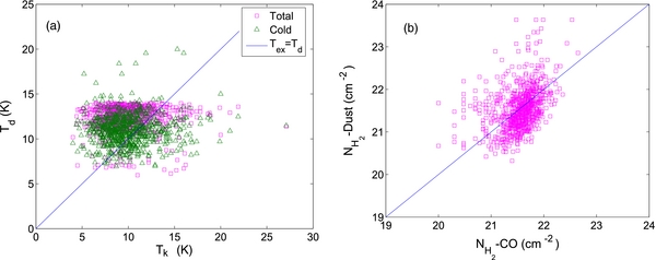
Figure 12. Comparison of Tk to Td and  to that deduced from dust emission.
Download figure:
Standard image High-resolution image4.8. Evolutional Phases—A Comparison to Different Star Formation Samples
To investigate the physical conditions and examine the possibility of stars forming in the cold clumps, we compare the line widths of 13CO (1–0) and column densities with the following CO molecular line surveys toward different kind of targets.
- 1.Methanol maser sources (Liu et al. 2010),
- 2.
- 3.Candidates of extremely young stellar objects chosen with a redder color IRAS index and smaller flux density than those of UC H ii regions (Wang et al. 2009),
- 4.IRDCs (Simon et al. 2006), and
- 5.Extended green objects (EGOs) identified from the Spitzer GLIMPSE survey (Chen et al. 2010).
Figure 13(a) plots a cumulative fraction of the FWHM of 13CO (1–0). It shows that the methanol maser sources have the largest FWHMs and the smallest slopes. The IRDCs and EGOs have a shape similar to the methanol maser sources but with slightly larger slopes. When the FWHM is less than 3 km s−1, the slope of IRDCs is almost the same as those of the UC H ii candidates and the redder, weaker IRAS sources. When the FWHM becomes larger than 3 km s−1, the changes of the UC H ii candidates and the redder, weaker IRAS sources are much steeper than IRDCs, EGOs, and the methanol maser sources. The slope of the fraction of the redder, weaker IRAS is large and its maximum value is at 6 km s−1. The variation of the cumulative fraction function of FWHM for the Planck cold clumps is the narrowest. The FWHM of the Planck cold clumps are the smallest compared with the other samples. For all the samples used in the comparison with Planck cold clumps, their FWHMs are almost larger than 2 km s−1 while the cumulative fraction at FWHM > 2 km s−1 of the cold clumps is less than 10%.
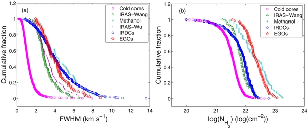
Figure 13. Comparisons for the cumulative fraction of the FWHM of 13CO lines and  of different star formation samples.
Download figure:
Standard image High-resolution imageThe comparison of column densities for the samples of (1), (3), (4), and (5) is presented in Figure 13(b). The cumulative fraction distribution also produces the smallest column density range for the Planck cold clumps. IRDCs have nearly the same shape as Planck cold clumps when the column density is below 1021 cm−2, but are similar to the redder, weaker IRAS sources at high densities, indicating that IRDCs may be at a transition phase between Planck cold clumps and redder, weaker IRAS sources. The methanal maser sources and EGOs have the largest column densities, indicating active star formations in them.
These results show that the Planck cold clumps are quiescent and have the smallest column densities among these star formation samples on the whole. Most of them seem to be in transition from clouds to dense clumps.
5. SUMMARY
Aiming to understand gas properties of the Planck cold dust clumps, we have carried out a survey for ECC clumps with J = 1–0 lines of 12CO, 13CO, and C18O. Using the 13.7 m telescope of PMO, 674 clumps were observed. Their observed parameters Vlsr, FWHM, and antenna temperature were presented. Distances and physical parameters Tex, velocity dispersions, and  were derived, and their spatial distribution, regional difference, and environmental effect were investigated. Ten clumps were mapped and their morphologies and properties were analyzed. Evolutionary states of the cold clumps were discussed when compared with different star formation samples. Our main findings are as follows.
- 1.With the survey of the 673 clumps, 782 13CO emission components were identified. Of these, 437 components had detection of all three transitions. Line center velocity differences for V12 − V13 of 94% of the clumps and for V13 − V18 of 98% of the clumps are less than 3σ of the velocity resolution. The correlations between the V12 and V13, V13 and V18 have ∼100% confidence. This is the first time the agreement of the velocities of 12CO and its major isotopes, the 13CO and C18O lines, has been confirmed with such a large sample. This suggests that the Planck clumps are quite cold and uniform as a whole and have no significant differences in dynamical or thermal material layer structures.
- 2.For each of the identified components, kinematic distance, galactocentric distance, and altitude from the Galactic plane were derived. The distance ranges from 0.1 to 21.6 kpc; 82% of them are located within 2 kpc and 51% of the components have distances within 0.5 and 1.5 kpc.
- 3.The mean value of the 12CO antenna temperature T12 is 3.08 ± 1.37 K. The mean ratio of T12/T13 is 2.15 ± 1.35 and T13/T18 is 3.88 ± 1.71. Excitation temperature ranges from 3.9 to 27.0 K. Ninety-eight percent of the clumps have Tex (or Tk under LTE assumption) smaller than 17 K. A comparison of the Tk and Td shows that most of the clumps have Td > Tk suggesting that gas could be heated via collision with dust and that dust and gas are coupled well in 95% of the clumps. There are clumps with Tk > 17 K, which are located in star formation regions such as Orion and Taurus, suggesting that the high Tk is related to star-forming activities.
- 4.The mean FWHMs of the three transitions J = 1–0 lines of 12CO, 13CO, and C18O are 2.03 ± 1.28, 1.27 ± 0.77, and 0.76 ± 0.75, respectively. Adopting 1.3 km s−1 of the FWHM of the 13CO (1–0) lines as a criterion of high- or low-mass clumps, ∼75% belong to the L group, suggests that the majority of the ECC clumps are low-mass clumps. For the 13CO lines the 3D velocity dispersion σ3D and nonthermal velocity dispersion σNT were calculated and we found that nonthermal the motion is the dominant line broadening.
- 5.Column densities of the 13CO and C18O lines were derived. They span from 1014 to 1016 cm−2, which is about a critical value for collapse. The ratio of [X13]/[X18] has a mean value of 7.0 ± 3.8, higher than the terrestrial value. Hydrogen molecule column densities were obtained for 782 13CO components, which are from 1020 to 4.5 × 1022 cm−2. Column densities derived from CO observations cover a narrower range than those deduced from dust emission.
- 6.Histograms for the antenna temperature T12, the ratio of T12/T13, T13/T18, excitation temperature Tex, and the velocity dispersions (σ3D, σNT, and ratio of σNT/σtherm) as well as τ13, [X13]/[X18], and
 were fitted with a lognormal distribution. The distributions of line widths of the three transitions, T13/T18, Tex, σ3D, σNT, σNT/σtherm, and [X13]/[X18] can be well depicted purely by a lognormal distribution. The lognormal distribution of the H2 column density is with a long tail which is consistent with those found in active star-forming regions, indicating that some of the Planck cold clumps reside in star-forming regions. We suggest the distributions of line widths or velocity dispersions are more likely to reflect the effect of supersonic turbulence in clouds.
 - 7.Physical parameter variations in Galactic space were investigated. As a variation with radius the hydrogen molecule column density reaches maximum at R ∼ 5 kpc, which is consistent with the 857 GHz flux density. However, τ13 decreases to a low valley while the σNT or σ3D reaches a peak. The results suggest that the velocity dispersion of the molecular line is the dominant factor in determining the column density. Velocity dispersions decrease as the altitude increases and they reach their lowest point at Z = 450 pc. Although τ13 is at its highest value here, the column density is at a low valley, further conforming that nonthermal line broadening plays a major role in exciting the molecular transition.
- 8.Line profile characteristics including a possible depletion dip, blue and red profiles, as well as high velocity wings were found in part of the clumps, indicating star-forming activities. However, the number of these clumps is less than 10% of the whole sample, indicating that star formation is not yet active in Planck cold clumps.
- 9.Parameters in different molecular complexes in our Galaxy show different scores. Clumps in the molecular complexes Ophiuchus, Taurus, and Orion show high excitation temperatures while those in the first–fourth quadrants have larger velocity dispersions.
- 10.Ten mapped cold dust clumps have very different gas emission morphologies, showing filaments or elongated structures. Twenty-two gas cores were identified with sizes of a tenth to 5 pc, densities from 102 to 103 cm−3 and masses from dozens to thousands of M☉. Ten cores seem to be in a gravitationally bound state.
- 11.Planck cold clumps are the most quiescent ones among the samples of weak red IRAS, UC H ii candidates, IRDCs, EGOs, and methanol maser sources, suggesting that the Planck cold clumps are at a very early phase in cloud evolution.

This work is a preliminary investigation for Planck cold clumps. Mapping observations are necessary for obtaining the properties of the Planck clumps. Various molecular species, especially dense molecular tracers, are needed for examining dense clumps and star formation processes in the ECC clumps. Mapping with H i line in ECC clumps is useful to investigate the transition from diffuse to dense ISM.
We are grateful to the staff at the Qinghai Station of PMO for their assistance during the observations. We thank the Key Laboratory for Radio Astronomy, CAS, for partial support in the operation of the telescope. This work was supported by China Ministry of Science and Technology under State Key Development Program for Basic Research (2012CB821800).