


ABSTRACT
Methanol (CH3OH) radiates efficiently at infrared wavelengths, dominating the C–H stretching region in comets, yet inadequate quantum-mechanical models have imposed limits on the practical use of its emission spectra. Accordingly, we constructed a new line-by-line model for the ν3 fundamental band of methanol at 2844 cm−1 (3.52 μm) and applied it to interpret cometary fluorescence spectra. The new model permits accurate synthesis of line-by-line spectra for a wide range of rotational temperatures, ranging from 10 K to more than 400 K. We validated the model by comparing simulations of CH3OH fluorescent emission with measured spectra of three comets (C/2001 A2 LINEAR, C/2004 Q2 Machholz and 8P/Tuttle) acquired with high-resolution infrared spectrometers at high-altitude sites. The new model accurately describes the complex emission spectrum of the ν3 band, providing distinct rotational temperatures and production rates at greatly improved confidence levels compared with results derived from earlier fluorescence models. The new model reconciles production rates measured at infrared and radio wavelengths in C/2001 A2 (LINEAR). Methanol can now be quantified with unprecedented precision and accuracy in astrophysical sources through high-dispersion spectroscopy at infrared wavelengths.
Export citation and abstract BibTeX RIS
1. INTRODUCTION
Modeling the spectroscopic properties of methanol (CH3OH) is particularly challenging because of the molecule's hindered internal rotation and asymmetric structure. Since the initial radio detection of interstellar methanol (toward the Galactic center; Ball et al. 1970), this astrochemically relevant compound has been detected in extremely diverse environments, from the interstellar medium (e.g., Johansson et al. 1984) to cometary atmospheres (e.g., Bockelée-Morvan et al. 1991; Hoban et al. 1991).
Because methanol has intense rotational and torsional spectra, most studies have been performed at microwave and far-infrared wavelengths and their successes have prompted spectroscopists to characterize the low-lying torsional–rotational energies with high accuracy. The latest compilation by Xu et al. (2008) describes the first three torsional levels of the ground vibrational state with excellent precision, although their analysis is based on an extremely complex Hamiltonian containing a large number (119) of spectroscopic parameters. Understanding of the intrinsic radiative properties of CH3OH at infrared wavelengths has progressed more slowly, owing to the greater density of overlapping rotation–torsion–vibrational lines and complex network of interactions.
Line-by-line rotationally resolved infrared spectra of methanol in natural sources are now in hand, thanks to recent advances in infrared detectors and powerful high-resolution spectrometers operating at high-altitude observatories. Most models for cometary methanol are based on integrated band intensities measured in the early 1980s (e.g., Rogers 1980). Until relatively recently, quantum assignments for individual lines within the three CH-stretch fundamental bands (ν2, ν3, and ν9) in the main spectral region (2–5 μm) accessed by most infrared spectrometers were restricted to a relatively small number of individual lines (e.g., Xu et al. 1997). Making unambiguous and complete quantum assignments for individual lines was particularly challenging (Hunt et al. 1991; Bignall et al. 1994; Xu et al. 1997) owing to their high line density (thousands of lines) in the wavelength range from 3.35 to 3.6 μm, complicated by the fact that accurate modeling of rotation–torsion–vibrational energies requires a Hamiltonian that takes into account the strong interactions between these small amplitude vibrations and torsional and low-lying vibrational bath states. The detailed work of Xu et al. (1997) for the ν2 band also revealed strong mixing with "dark" background bath states and intense perturbations that made the modeling of these band systems impractical and virtually unattainable.
The first attempts to model these band systems for interpreting low-resolution spectra (λ/Δλ ∼ 1000) used the known ground-state rotational constants for the upper vibrational states, and neglected molecular asymmetry and internal rotation (Hoban et al. 1991; Reuter 1992; Bockelée-Morvan et al. 1995). Nevertheless, these pioneering works led to an improved understanding of this spectral region in comets, and fluorescence efficiencies calculated with these models are used today to retrieve abundances of cometary methanol. However, their limitations are revealed at higher resolving powers (λ/Δλ > 104), where they fail to describe the general morphology of the observed spectra (e.g., see Figure 1(b) in DiSanti et al. 2009). Moreover, the emergence of competing fluorescence models for the ν3 band led to highly inconsistent (model-dependent) abundances for methanol in comets, even when different investigators sampled the same spectral regions in the same comet (e.g., compare Mumma et al. 2011; Dello Russo et al. 2011). The measured fluxes were in agreement, but the models used to interpret them were not.
In this paper, we present a new quantum-mechanical model for the ν3 band of methanol, incorporating the latest experimental band intensities and a practical treatment of the different torsional species. We also include torsional and vibrational hot bands identified from laboratory experiments, and consider an accurate treatment of rotational, torsional, and vibrational partition functions for the 10–400 K regime (appropriate for atmospheres of comets and several planets, including Mars). The new band system was integrated into our general fluorescence model (GFM; Villanueva et al. 2011) to synthesize non-LTE cometary spectra and was then used to interpret high-resolution spectra of three comets: C/2001 A2 LINEAR, C/2004 Q2 Machholz, and 8P/Tuttle. The cometary data sets provide a stringent test of the newly developed line-by-line fluorescence model, since they are of high spectral quality (λ/Δλ up to 98,000, acquired with CRIRES/VLT and NIRSPEC/Keck II) and they sample a range of rotational temperatures.
2. THE ν3 BAND MODEL OF METHANOL
Methanol is a slightly asymmetric molecule with a plane of symmetry and has been historically associated with the Cs point group, with in-plane and out-of-plane symmetry modes (A' and A''). On the other hand, when the effects of torsional tunneling are included, the molecule is better described with the permutation-inversion point group (G6), isomorphic to C3V, with three representations (Γ = A1, A2, and E). When modeling methanol spectra, different authors have considered alternative point groups or adopted differing notations, further complicating the compilation and integration of previous results. Some groups even neglect the torsional labeling and use the standard asymmetric top notation for the levels (J, Ka, and Kc), while others include torsional symmetry as well as torsional state in the notation (νt, τ, K, J)v, where νt denotes the torsional state, v the small amplitude vibrations, and τ = 1, 2, 3 the torsional species. Another common methanol notation used is (νt, K, Ts, J)v, where Ts represents torsional symmetry of A, E1, and E2.
In this paper, we use the C3v point group and the notation adopted in most recent methanol publications (e.g., Xu et al. 1997, 2008). Rotational levels are described with three quantum numbers: J as the total angular momentum (J ⩾ 0), K as its projection along the symmetry a-axis (0 ⩽ K ⩽ J), and TS as the torsional symmetry: A, E1, E2. The A states are further split for K > 0 due to the molecular asymmetry and are labeled as A+ and A−. Some authors (e.g., Mekhtiev et al. 1999) differentiate between the E1 and E2 states by using signed K values with +K E levels being E1 and −K E levels being E2.
2.1. Torsional–Rotational Energies
For the ground vibrational state (Figure 1), we adopted the energies E''(J, K, Ts) reported by Mekhtiev et al. (1999) and Xu et al. (2008), and used them to estimate the parameters for the upper vibrational state (ν3). Using the ν3 parameters reported by Hunt et al. (1991) for some K sub-bands, and additional line identifications determined by Xu, we searched for deviations of the energy structure with respect to the ground state, and created progressions according to τ leading to slower and smoother variation with K. The torsional index (τ = 1, 2, 3) is related to the aforementioned torsional symmetry Ts by the following rule: mod(K + τ)/3 = 0 for E1, 1 for A, and 2 for E2. The torsional index (τ), associated with symmetry, should not be confused with the torsional quantum number (νt). The torsional energies for the ground state (Figure 2) were estimated using the following relation:
where A, B, and C are the main rotational constants for the ground vibrational state (A = 4.2537233, B = 0.8236523, C = 0.7925575; Xu et al. 2008). This approximation neglects high-order effects and perturbations, but it does provide a useful representation of the general variations of energy for each torsional mode (Figure 2). We obtained experimental fits to the torsional energies, in a fashion similar to that of Wang & Perry (1998), using

where c0–4 are the five coefficients describing the torsional energy pattern. Using this equation and considering all torsional sub-bands having K ⩽ 17, we derived the five constants of Equation (2) (c0–4; see Table 2). The values are defined with respect to the bottom of the potential well, which (following Mekhtiev et al. 1999) we consider to be 128.10687 cm‑1 below the first rotational level (J = 0, K = 0, A+).
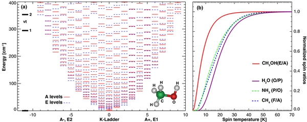
Figure 1. Rotational and symmetry structure of the ground vibrational level of CH3OH. (a) Rotational structure for the lower torsional state (νt = 0), with symmetries indicated by different trace types and colors. (b) Symmetry ratio of methanol (A = A+ + A−, E = E1 + E2) in comparison to water (H2O, O/P = 3 at eq.), ammonia (NH3, P/O = 1 at eq.), and methane (CH4, F/A = 9/5 at eq.).
Download figure:
Standard image High-resolution image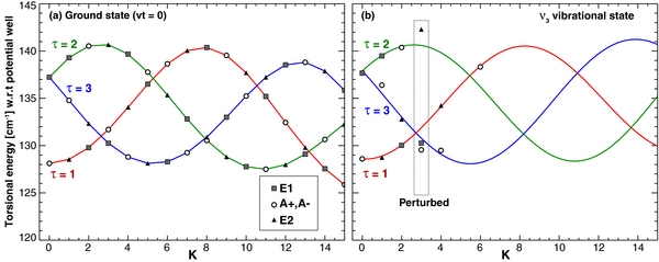
Figure 2. Torsional energy diagrams for the ground and ν3 (2844.2 cm−1) vibrational states. The torsional energies were derived using Equation (1), with values for the ground state from Mekhtiev et al. (1999) and Xu et al. (2008), and considering 709 line identifications for the ν3 band. The torsional modes of the ν3 state were fitted using Equation (2) (see Section 2.1).
Download figure:
Standard image High-resolution imageFor the upper vibrational state, we created differential progressions in J for every K sub-band based on experimental data and extrapolated to other sub-bands using the torsional diagram. The differential progressions are defined as
where ν0 is the band center (2844.2 cm−1), δν is the torsional displacement of the K sub-band with respect to the torsional–rotational energy of the same K sub-band in the ground state, and δB is the differential rotational constant for a K sub-band. Using 709 ro-vibrational assignments of the ν3 band, we retrieved 19 origins and 19 differential rotational constants for sub-bands with K' ⩽ 6 (see Table 1). For all other K sub-bands (marked with an asterisk ''*'' in Table 1), δB was set to ‑0.0048371871, which is the median of the 19 extracted values.
Table 1. List of Parameters Relevant to Differential Torsional Energies of the ν3 Vibrational State with respect to the Ground Vibrational State (see Equation (3))
| K' | E1 | A+ | A− | E2 | |
|---|---|---|---|---|---|
| 0 | δν | 0.472427 | 0.515070 | ||
| δB | −0.000163 | −0.002999 | |||
| 1 | δν | 0.232969 | 1.644089 | 1.648615 | 0.240550 |
| δB | −0.002845 | 0.001430 | −0.012424 | −0.016448 | |
| 2 | δν | 0.283519 | −0.109288 | −0.117130 | 0.495529 |
| δB | −0.010409 | −0.004837 | −0.004596 | −0.006310 | |
| 3 | δν | 0.053291 | −2.106990 | −2.111880 | 1.663912 |
| δB | −0.004447 | −0.005146 | −0.005093 | −0.008170 | |
| 4 | δν | 0.189937* | 0.730155 | 0.730167 | 0.225078 |
| δB | −0.004837* | −0.007722 | −0.007725 | 0.007489 | |
| 5 | δν | −0.069808* | 0.565761* | 0.565761* | 0.104760* |
| δB | −0.004837* | −0.004837* | −0.004837* | −0.004837* | |
| 6 | δν | −0.046387* | −0.264249 | −0.281261 | 0.911340* |
| δB | −0.004837* | −0.001436 | −0.001261 | −0.004837* | |
| 7 | δν | 1.104191* | −0.092171* | −0.092171* | −0.160811* |
| δB | −0.004837* | −0.004837* | −0.004837* | −0.004837* | |
Notes. δν is the torsional displacement of the K sub-band with respect to the torsional–rotational energy of the same K sub-band in the ground state, and δB is the differential rotational constant for a K sub-band. The torsional mode (τ) is indicated with the background color (τ = 1, dark gray; τ = 2, light gray; τ = 3, white). Coefficients calculated following the torsional diagram (see Figure 2 and Section 2.1) are indicated with an asterisk ''*,'' while the remaining values have been derived following Equation (3) and using new line IDs and including certain identifications presented by Hunt et al. (1991).
Download table as: ASCIITypeset image
The definition of δν beyond the measured sub-bands is extremely difficult without a full Hamiltonian that includes perturbations and interactions with other vibrational and torsional states. In addition, the empirical data are limited to values that span K' ⩽ 6, and some of the measurements indicate strong perturbations (e.g., K' = 3). We extrapolated to other K ladders, by fitting the five coefficients (c0–4; see Equation (2)) of the torsional diagram to the measured torsional band centers (δν, see Table 2). In the fit, we excluded the perturbed values for K' = 3. We thus define the torsional–rotational displacement for those K sub-bands having no experimental data to be δν = E'tors–E''tors, where E'tors was calculated using Equation (2) with (fitted) c0–4. E''tors was calculated using Equation (1) with values from Mekhtiev et al. (1999) and Xu et al. (2008). See synthetic spectra and energy spectral distribution at 100 K in Figure 3.
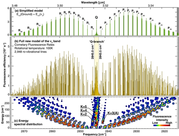
Figure 3. Fully resolved model of the ν3 band of methanol and its spectral energy distribution at 100 K. (a) A simplified band model calculated by assuming the rotational structure of the ν3 vibrational state to be the same as the ground vibrational state (Hoban et al. 1991; Reuter 1992; Bockelée-Morvan et al. 1995). (b) Fully resolved and line-by-line fluorescence efficiencies for 2948 ro-vibrational lines using the new model. Fluorescence efficiencies for the region marked as ''Q-branch'' (2843.5–2845.0 cm−1) are listed in Table 3 for a set of five temperatures. (c) Modeled emission for the ν3 band of methanol at 100 K organized by the corresponding lower state energy (y-axis), and color-coded by intensity. The labels K = 2, 3, 4, 5 indicate the position of the K-ladders component of the Q-branch (ΔJ = 0). The map has been smoothed to improve its clarity.
Download figure:
Standard image High-resolution imageTable 2. Harmonic Torsional Constants (see Equation (2)) for the Ground and ν3 Vibrational States of Methanol
| c0 | c1 | c2 | c3 | c4 | |
|---|---|---|---|---|---|
| Ground | 133.84356 | 0.23722 | 0.027307 | −6.1352 | 0.39735 |
| ν3 | 134.83284 | −0.16811 | 0.013409 | −6.2039 | 0.38327 |
Download table as: ASCIITypeset image
2.2. Partition Functions
Even though great advances have been made in characterizing the energy structure of methanol, current spectroscopic databases differ greatly in their description of the partition functions, and this could ultimately lead to significant errors in the computed band intensities. For example, the HITRAN database tabulates Ztot = 82,469 at 296 K in the total partition table (''parsum.dat''), and 35,314 at 296 K in the molecular table (''molparam.txt''). At 300 K, the JPL Molecular Spectroscopy database for methanol (Pearson & Xu 2010) reports Ztot = 37,892 (after correcting for a spin multiplicity of 4), while the analytical method of Dang-Nhu et al. (1990) estimates Ztot = 35,065 at 296 K. Furthermore, none of these sources lists partition functions at 1 K intervals in the 10–400 K temperature range, required for computing fluorescence efficiencies for comets and absorption coefficients for planetary atmospheres. We found the method of Dang-Nhu et al. (1990) to be appealing because of its simplicity and possible high-dynamic range. Nevertheless, when we compared results obtained using this method with values derived using more rigorous calculations, we were discouraged by the large differences, in particular in the low temperature range.
In order to compute partition functions we combined the energy characterization obtained by Mekhtiev et al. (1999) for the ground state (which spans νt ⩽ 8 and J ⩽ 22) with a simplified Hamiltonian for high energies (J > 22). We assumed that the torsional–rotational structure of the ground state also applies to all other vibrational modes (see vibrational energies in Dang-Nhu et al. 1990) and that the rotational levels with J > 22 follow the progression listed in Equation (1). Using this method we created 2,193,894 levels (νt ⩽ 8 and J ⩽ 100), in addition to the 9522 levels listed in Mekhtiev et al. (1999), and we computed the partition function by explicitly summing over all energy levels generated by this calculation (Table 3). Our partition functions are in excellent agreement with the latest numbers given by Pearson & Xu 2010 (see revision after 2011 November, now listed on the JPL Molecular Spectroscopy Web site)—the differences are typically smaller than 0.2% (Figure 4).
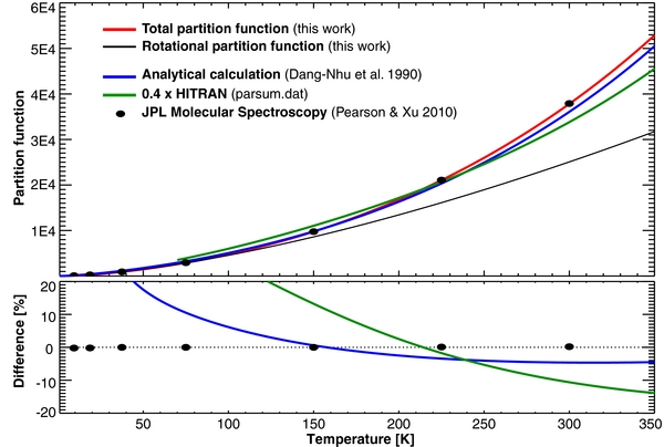
Figure 4. Comparison of partition functions for methanol from various authors. In general, the analytical method of Dang-Nhu et al. (1990) provides practical accuracy (|δ| < 5%) for temperatures above 120 K, while we obtain excellent agreement with the latest values reported by Pearson & Xu (2010; revised values after 2011 November, as now given in the JPL Molecular Spectroscopy database).
Download figure:
Standard image High-resolution imageTable 3. Spectroscopic Parameters of the ν3 Band of Methanol
| Parameter | Value | Unit | ||
|---|---|---|---|---|
| C–H integrated intensity at 25°C (298.15 K) | ν3 | 22% | ||
| Spectral range: 2650–3175 cm–1 | ν9 | 50% | 211 | 10–19 cm molecule–1 |
| Rogers 1980 | ν2 | 28% | ||
| C–H integrated intensity at 296 K | ||||
| Spectral range: 2650–3175 cm–1 | 211 | 10–19 cm molecule–1 | ||
| PNNL Spectral database (Sharpe & Sams 2000) | ||||
| Torsional partition function at 296 K | 1.46800 | |||
| Vibrational partition function at 296 K | 1.01971 | |||
| Total partition function at 296 K | 36761 | |||
| ν3 band intensity at 296 K | 31.01 | 10–19 cm molecule–1 | ||
| 75 K | 143.4 | |||
| ν3 band fluorescence efficiency | 150 K | 128.4 | 10–6 s–1 | |
| 296 K | 97.3 | |||
| 10 K | 12.9 | |||
| g-Factor of the ν3 Q-branch | 40 K | 14.4 | ||
| Range: 2843.5–2845.0 cm–1 | 75 K | 15.5 | 10–6 s–1 | |
| 100 K | 15.5 | |||
| 130 K | 14.6 | |||
Notes. Fluorescence efficiencies are in units of photons molecule−1 s−1 at heliocentric distance 1 AU.
Download table as: ASCIITypeset image
2.3. Line Intensities and Einstein A21 Coefficients
The most recent report of the integrated intensity for the ν3 band of methanol is more than 30 years old, when Rogers (1980) performed a comprehensive study of infrared intensities of alcohols and ethers. Band intensities from this work were used by Reuter (1992) and Bockelée-Morvan et al. (1995; referred to as BM95 hereafter) to derive cometary fluorescence efficiencies, although the authors differ in their integrated fluorescence efficiencies (gband) by ∼20%. Considering the formalism by Crovisier & Encrenaz (1983), we derive gband = 1.47 × 10⁻⁴ s−1, consistent with the value presented in BM95. However, the derivation of the intensity of the ν3 fundamental presented in BM95 is only valid for the low temperatures (T < 100 K) typically measured in comets, i.e., for temperatures at which torsional and vibrational excitations (and thus hot bands) are negligible (see below).
The laboratory measurements of Rogers (1980) consisted of integrating over the complete C–H stretching region (2650–3175 cm−1), which was further divided into the different vibrational modes (ν2, ν3, ν9) by considering the following relative contributions: fν = 28%, 22%, 50%, respectively. We compared the C–H value in Rogers (1980) (127 ± 10 (km mol−1) or 211 × 10−19 (cm molecule−1)) with recently calibrated spectra (Sharpe & Sams 2000) of the Pacific Northwest National Laboratory (PNNL) and obtained excellent agreement (Table 3). However, these laboratory measurements were performed at room temperature, where torsional and hot bands are particularly active and therefore contribute significantly to the observed intensities. The first torsional state lies just 294.45 cm−1 above the ground state. From our partition function calculations, we estimate the contribution of hot bands to be fhot = 33% at 296 K, similar to the findings of 31% by Xu et al. (2004) for the C–O stretching region. Taking the intrinsic intensity of the hot bands to be the same as the fundamental, the contribution of the hot bands is estimated to be fhot = 1–(ZvibZtors)−1. Accordingly, we estimate the intensity of the ν3 fundamental to be Sv3(296 K) = (fv3SCH)(1 − fhot) = 31 × 10−19 (cm molecule−1); see Table 3.
We computed line intensities (Sv) for all allowed transitions connecting upper and lower states (ΔJ = J'–J'' = +1, 0, ‑1; ΔK = 0; A ± ↔ A± (ΔJ ≠ 0), A± ↔ A ∓ (ΔJ = 0), E ↔ E) as follows:
where ν is the line frequency (E'–E'' (cm−1)), LHL is the Hönl–London factor, w'' is the statistical weight of lower state (=4(2J''+1), including the spin multiplicity of 4), and Zrot(T) is the rotational partition function (24,558 at 296 K). The Hönl–London factors for a parallel band are defined as (Herzberg 1945, p. 422):
This approximation for the computation of line intensities neglects high-order interactions coupling torsional and vibrational modes, which have been reported to be active in the 3 μm spectral region (Brooke et al. 2003; Xu et al. 1997). Einstein-A coefficients were computed following Šimečková et al. (2006):

where Ztot(T) is the total internal partition sum (36,761 at 296 K), Ia is the isotopic abundance (Ia = 0.98593 for normal CH3OH), and w' is the statistical weight of the upper state.
2.4. Machine Readable Spectral Atlas
Following the above guidelines, we computed 2948 spectral lines with Jmax = 23 in the 2802 cm−1 to 2892 cm−1 frequency range. The database has been organized according to the HITRAN 2008 format with line identifications following the G6 point group model, which is accessible by our GFM and planetary radiative transfer models (LBLRTM and MRTM; Clough et al. 2005; Villanueva et al. 2011). The vibrational indicators are V3, GROUND; while the local quantum numbers are J, K, and TS. Line shape coefficients were defined following Xu et al. (2004): air-broadened half-width γair = 0.100 cm−1 atm−1, self-broadened half-width γself = 0.400 cm−1 atm−1, temperature-dependence exponent ηair = 0.75, and pressure-induced line shift δair = 0.00 cm−1 atm−1.
3. APPLICATION OF THE MODEL TO MEASURED COMETARY SPECTRA
The CH3OH ν3 band is particularly bright in hydrocarbon-rich comets where efficient solar pumping and inefficient collisional quenching lead to strong methanol fluorescent emission. At 300 K, the ν3 band is so complex as to defy development of comprehensive structural models, but this complexity is greatly reduced at lower rotational temperatures permitting development of the new model described herein.
Collision partners in cometary atmospheres usually lack sufficient kinetic energy to excite vibrational transitions, and the rate of quenching collisions is much smaller than radiative decay rates for (infrared active) excited states. For these reasons, the vibrational manifold is not significantly populated in LTE. Instead, solar radiation pumps the molecules into excited vibrational states, which subsequently de-excite by rapid radiative decay. Infrared photons are emitted through decay to the ground vibrational state, either directly (through resonant fluorescence) or through branching into intermediate vibrational levels (non-resonant fluorescence). Resonant fluorescence is expected to be the dominant factor in the excitation of the ν3 band, and it is the sole pumping mechanism considered here, although additional excitation cascading from levels with energies higher than ν3 may also be active.
We derived a new CH3OH line atlas from our newly developed methanol quantum band model and integrated it into our GFM (Villanueva et al. 2011) to synthesize cometary emission spectra. For a realistic description of the solar spectrum, we earlier developed a model that combines a contemporary continuum model (Kurucz 2009) and an accurate solar line atlas (Hase et al. 2006) modulated by Doppler broadening introduced by differential solar rotation (see Appendix B of Villanueva et al. 2011). In Figure 3, we show the fluorescence spectrum synthesized for CH3OH at a rotational temperature of 100 K to illustrate these points.
Measured rotational temperatures for primary volatiles in comets can range from ∼15 K to ∼140 K, so comparing simulated and measured fluorescent emission spectra can provide a critical test of our new ν3 band model. To that end, we next compare synthetic and measured spectra of three Oort cloud comets (C/2001 A2 (LINEAR), C/2004 Q2 (Machholz), and 8P/Tuttle (now in a Halley-type orbit)). We also compare revised and published production rates and mixing ratios (relative to water) for these three comets and for 103P/Hartley 2—an ecliptic comet now in Jupiter's dynamical family but originally from the Kuiper Belt reservoir.
3.1. Comet C/2001 A2 (LINEAR)
We applied our quantum band model to high-resolution (λ/Δλ ∼ 25,000) infrared spectra of comet C/2001 A2 (LINEAR) (A2 hereafter), acquired in 2001 July with NIRSPEC (Near-InfraRed Echelle SPECtrograph; McLean et al. 1998) at the Keck II Telescope in Hawaii. In 2001 July, comet A2 displayed intense lines of CH3OH (Figure 5), owing to its particularly rich organic chemistry (Magee-Sauer et al. 2008). The abundances of ethane, acetylene, hydrogen cyanide, and methanol were enriched by factors of 2–3 with respect to most comets in our database (e.g., Mumma & Charnley 2011; DiSanti & Mumma 2008).
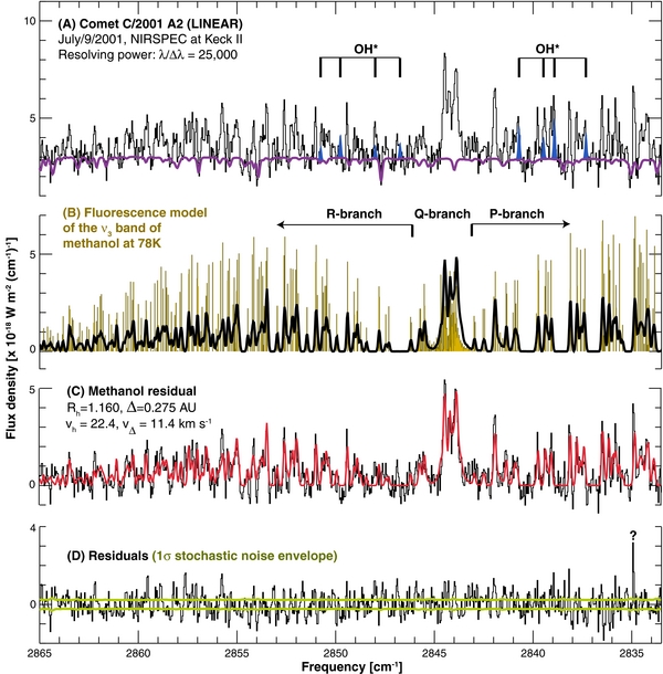
Figure 5. Comparison of measured and modeled spectra of methanol in comet C/2001 A2 (LINEAR). Measurements were acquired on 2001 July 9 UT using NIRSPEC at Keck-II (Magee-Sauer et al. 2008). (A) The upper trace shows a spectrum extracted from the sum of nine spatial rows centered on the comet nucleus (a model of the cometary dust continuum affected by terrestrial transmittance is overlaid). The positions of several OH multiplets are marked. Their difference (trace C) after OH removal reveals the residual methanol emission (ν3 band) from the comet, as affected by terrestrial atmospheric transmittance. (B) The line-by-line modeled stick spectrum (yellow) is compared with the convolved methanol emission (black). (C) The line-by-line modeled spectrum convolved to the instrumental resolution is compared with the measured emission spectrum. (D) Residuals after subtracting the new (convolved) methanol model from the measured spectrum.
Download figure:
Standard image High-resolution imageFrom A2 spectra acquired on 2001 July UT 9.5, we retrieved a global production rate [Q(CH3OH)] of (11.3 ± 0.04) × 1026 s−1 and a rotational temperature of 78 ± 5 K (using a chi-square minimization technique). The revised production rate is smaller by about 20% than the published value of (14.5 ± 0.4) × 1026 s−1 (Magee-Sauer et al. 2008), owing mainly to the revised g-factor for the integrated Q-branch. A re-analysis of the H2O, C2H6, and HCN spectra using our new analytical methods, reveals similar temperatures (Trot near 80 K) for these three species and consistent with the methanol value. Further details on the application of our new water model to this data set will be discussed elsewhere.
Our new production rate (Table 4) is very consistent with the value retrieved the previous night (2001 July UT 8.3) through radio observations (Biver et al. 2006), further validating our revised analytical methodology for computing non-LTE fluorescence efficiencies for this IR band system. We also explored the possibility of retrieving the nuclear spin temperature (Tspin) from these data, but uncertainties in line-by-line intensities introduced by the symmetric rotor approximation and by current unknowns of the CH3OH energy structure for K > 6 could introduce systematic uncertainties associated with such retrievals. Formally, our results indicate Tspin > 18 K for CH3OH, consistent with the findings of Tspin = 23+4−3 K for H2O in comet A2 (Dello Russo et al. 2005), and with Tspin derived for methanol in comet Hale–Bopp (Tspin > 15–18 K; Pardanaud et al. 2007).
Table 4. Methanol Abundances in Comets Retrieved Using the New Quantum Model of the ν3 Band
| Date | Source | Q(H2O) | Original Q(CH3OH) | Original abundance | Revised Q(CH3OH) | Revised CH3OH Abundance |
|---|---|---|---|---|---|---|
| (×1028 mol s—1) | (×1027 mol s—1) | % w.r.t. H2O | (×1027 mol s—1) | (%) | ||
| C/2001 A2 (LINEAR): long-period comet (Oort Cloud) | ||||||
| 2001 Jul 8 | Radio(1) | 3.77 ± 0.34(2) | 1.12 ± 0.16 | 2.97 ± 0.43 | 2.97 ± 0.43 | |
| 2001 Jul 9 | IR(2) | 3.77 ± 0.34 | 1.45 ± 0.04 | 3.85 ± 0.11 | 1.13 ± 0.04 | 2.99 ± 0.11 |
| C/2004 Q2 (Machholz): long-period comet (Oort Cloud) | ||||||
| 2005 Jan 19 | IR(3) | 27.3 ± 0.70 | 6.20 ± 0.21 | 2.27 ± 0.08 | 4.20 ± 0.20 | 1.54 ± 0.07 |
| 2005 Jan 30 | IR(4) | 34.2 ± 1.90 | 4.01 ± 0.21 | 1.18 ± 0.06 | 5.61 ± 0.29 | 1.65 ± 0.09 |
| 8P/Tuttle: Halley-type short-period comet (Oort Cloud) | ||||||
| 2007 Dec 22 | IR(5) | 2.28 ± 0.05 | 0.50 ± 0.01 | 2.18 ± 0.05 | 0.44 ± 0.01 | 1.91 ± 0.04 |
| 2008 Jan 29 | IR(6) | 5.97 ± 0.27 | 2.00 ± 0.19 | 3.36 ± 0.32 | 1.50 ± 0.11 | 2.51 ± 0.19 |
| 2008 Feb 4 | IR(7) | 3.00 ± 0.20 | 0.97 ± 0.13 | 3.23 ± 0.44 | 0.76 ± 0.10 | 2.52 ± 0.34 |
| 103P/Hartley 2: ecliptic short-period comet (Kuiper belt) | ||||||
| 2010 Sep–Dec | IR(8) | 0.21–0.77 | 0.06–0.20 | 2.77 ± 0.19 | 0.04–0.15 | 1.87 ± 0.13 |
| 2010 Nov 4 | IR(9) | 0.88–1.40 | 0.13–0.17 | 1.23 ± 0.08 | 0.18–0.24 | 1.72 ± 0.11 |
Notes. The sources of the data are: (1) Biver et al. (2006), (2) Magee-Sauer et al. (2008), (3) Bonev et al. (2009), (4) Kobayashi & Kawakita (2009), (5) Bonev et al. (2008), (6) Böhnhardt et al. (2008), (7) Kobayashi et al. (2010), (8) Mumma et al. (2011), and (9) Dello Russo et al. (2011).
Download table as: ASCIITypeset image
3.2. Comet C/2004 Q2 (Machholz)
Comet C/2004 Q2 (Machholz) (Q2 hereafter) was particularly active in 2005 January, with a very high water production rate (∼3 × 1029 mol s−1; Bonev et al. 2009; Kobayashi & Kawakita 2009). Like A2, Q2 presented a rich chemistry. On 2005 January 19, we obtained 8 minutes of integration with the KL1 setting of NIRSPEC, which samples the ν3 band of methanol in order 22. As shown in Figure 6, the methanol lines are noticeably strong and thus pose an excellent test for our newly developed model.
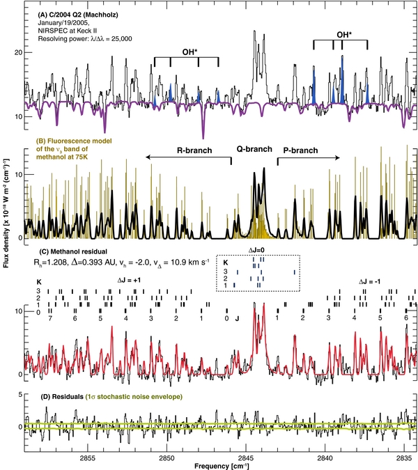
Figure 6. Comparison of the new methanol model and measured spectra of comet C/2004 Q2 (Machholz) taken on 2005 January 19 UT using NIRSPEC at Keck-II (Bonev et al. 2009). Line IDs (J'', K'') are presented in panel (C). Additional figure details are the same as in Figure 5.
Download figure:
Standard image High-resolution imageFor 2005 January 19, we retrieve a methanol production rate of (4.2 ± 0.2) × 1027 mol s−1 and a rotational temperature of 75 ± 5 K. The rotational temperature is similar to that derived for other molecules (78–83 K) by Kobayashi & Kawakita (2009). Considering the co-measured Q(H2O) derived by Bonev et al. (2009) of 2.7 × 1029 mol s−1, we obtain a methanol mixing ratio of 1.54% ± 0.07%. Kobayashi & Kawakita (2009) did not sample the ν3 band of methanol in their survey, but they retrieved methanol production rates from certain ν9 methanol features in the 2890–2934 cm−1 using empirical g-factors. The ν9 empirical g-factors were derived by scaling the observed fluxes measured in comet Lee (Dello Russo et al. 2006) and by considering a ν3 Q-branch g-factor of 2.17 × 10⁻⁵ s−1 derived from BM95. On the other hand, our new model predicts the g-factor of the ν3 Q-branch to be 1.55 × 10⁻⁵ s−1 at 70–80 K; see Table 3. The difference mainly originates because some K-ladders (e.g., K' = 3) are heavily perturbed and their Q-lines (ΔJ = 0) do not fall within the region normally defined as the Q-branch for this band system (2843.5–2845.0 cm−1). The fact that the new model considers a realistic torsional–rotational structure for the ν3 vibrational state solves this problem (see comparison in Figure 3 and line identifications in Figures 6 and 7). Correcting the methanol value reported by Kobayashi & Kawakita (2009) with a scaling factor of 1.4 (i.e., 2.17/1.55) brings their published mixing ratio (1.65% ± 0.09%) into agreement with our value (see Table 4).
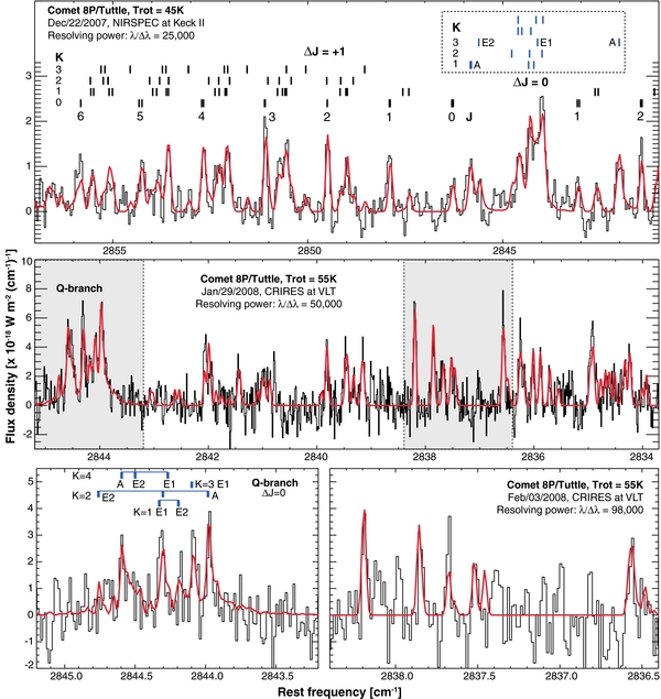
Figure 7. Comparison of the new methanol model and measured spectra of comet 8P/Tuttle obtained with different spectral resolutions.
Download figure:
Standard image High-resolution image
3.3. Comet 8P/Tuttle
The data available for comet 8P/Tuttle (8P hereafter) are extremely rich, since the comet was observed using two powerful high-resolution spectrometers (NIRSPEC/Keck II and CRIRES/VLT), by two independent teams and at different times during its apparition in 2007–2008. We re-processed our methanol data acquired with NIRSPEC (on 2007 December 22; Bonev et al. 2008) and CRIRES (on 2008 January 29; Böhnhardt et al. 2008), and compared the revised results with those acquired on 2008 February 4, with CRIRES (Kobayashi et al. 2010). The new model provides excellent agreement with 8P data recorded at high spectral resolutions (Figure 7), even when compared to data acquired using the narrowest slit in CRIRES (0.2''), which delivers an extremely high resolving power (λ/Δλ ∼ 98,000). Of particular significance is the high level of agreement between model and data near the Q-branch, which is the region used by astronomers to derive g-factors and whose differing models led to the disagreement among methanol values obtained for the same comet.
Our originally reported methanol production rates for 8P were reduced by ∼20% when the new model was applied, leading to a revised methanol abundance of 1.9%–2.5% with respect to water (see Table 4). The measurements of methanol by Kobayashi et al. (2010) targeted certain ν2 lines, but this time the empirical ν2 g-factors were scaled relative to the ν3 Q-branch after adopting a g-factor of 1.17 × 10⁻⁵ s−1 (DiSanti et al. 2009). Herewith they too should be revised downward by 20% (see Table 4). Their revised methanol abundance (2.52% ± 0.34%) then agrees very well with our value (2.51% ± 0.19%) measured a week earlier. The improved confidence levels (by removing modeling error) also suggest that the mixing ratio of methanol did change from December 22 to January 29.
3.4. Comet 103P/Hartley 2
The use of different g-factors to extract methanol abundances in comets became particularly problematic in 103P/Hartley 2, as two teams presented very different methanol abundances in this comet (Mumma et al. 2011; Dello Russo et al. 2011), even though most of the other abundances were consistent, and both teams used the same spectroscopic technique (NIRSPEC at Keck II) to sample methanol in this comet (ν3 band of methanol). As nicely summarized in Meech et al. (2011), the methanol abundances differed by a factor of ∼2. If we correct the abundances by applying the new g-factor for the methanol Q-branch of 1.55 × 10⁻⁵ s−1, both measurements now indicate a mixing ratio of ∼1.8% (see Table 4). More importantly, the new developed model not only brings consistency to the values of methanol measured in comets using different techniques and methods, but allows us to better understand this important spectral region (where many hydrocarbons are radiatively active) and it provides us with a robust tool to retrieve accurate rotational temperatures for this molecule from infrared spectra. The comparison of rotational temperatures among various species permits inferences regarding their common physical distributions and is needed when determining nuclear spin temperatures from the respective populations of individual nuclear spin species.
4. CONCLUSIONS
We constructed a line-by-line model for the ν3 band of methanol (CH3OH) and generated fluorescence efficiencies (g-factors) to retrieve methanol abundances in comets. The complex and spectrally dense rotational fine structure of the ν3-band system was described using a set of rotational constants for each torsional K-ladder, which includes a practical approximation of the three torsional modes of the ν3 vibrational level. The new band system, described with 2948 spectral lines, was integrated into our cometary GFM. The GFM includes a realistic solar pumping spectrum and a proper treatment of the Swings effect (a Doppler shift introduced by the comet's heliocentric (radial) velocity). Spectra synthesized with our methanol model agree very well with measured high-resolution spectra of three comets (A2, Q2, and 8P) recorded with NIRSPEC at Keck-II and CRIRES at VLT, and it reconciles radio and infrared production rates for methanol in C/2001 A2 (LINEAR). With the new model, highly accurate methanol production rates can be retrieved that are consistent with contemporaneous radio measurements.
Line lists and partition functions are available at http://astrobiology.gsfc.nasa.gov/Villanueva/spec.html.
G.L.V., M.A.D., and M.J.M. acknowledge support from NASA's Planetary Atmospheres and Astronomy Programs (08-PATM08-0031 (PI: G.L.V.), 09-PATM09-0080 (PI: M.A.D.), 08-PAST08-0033/34 (PI: M.J.M.), 09-PAST09-0034 (PI: M.A.D.)), NASA's Astrobiology Institute (NAI5/NNH08ZDA002C, PI: M.J.M.). L.H.X. gratefully acknowledges financial support from the Natural Sciences and Engineering Research Council of Canada. We thank Dr. Eva Wirström for helpful discussions.