


ABSTRACT
Using test-particle simulations, the off-diagonal elements of the diffusion tensor are evaluated numerically. The comparison of the so-obtained time-dependent drift coefficients with analytical approximations shows that, for weak turbulence strengths or for slab turbulence geometry, the weak scattering result provides an excellent agreement with the numerical results. For two- or three-dimensional turbulence geometry, however, neither the classical scattering result nor alternative analytical approaches provide an accurate description of the numerically obtained values. Furthermore, the influence is discussed of a non-constant energy range in the turbulence spectrum and of non-static turbulence, for which the time dependence is modeled using magnetohydrodynamic plasma waves.
Export citation and abstract BibTeX RIS
1. INTRODUCTION
Both astrophysical and laboratory plasmas are usually magnetized, with the magnetic field being composed of a mean component (often denoted as the "background" magnetic field or the guide field) and a turbulent component. In the astrophysical theater, such turbulence can be found for example in the solar system, where it is generated by the magnetized solar wind (e.g., Bruno & Carbone 2005), or in the interstellar medium, where the turbulent motion of gas clouds distorts the galactic magnetic field (e.g., Beck et al. 1996).
To describe the random motion of energetic charged particles parallel and perpendicular to a homogeneous magnetic field, several sophisticated nonlinear theories have been proposed in recent years, as is also the case for the diffusion of magnetic field lines. Examples are the second-order quasi-linear theory (Shalchi 2005; Tautz et al. 2008b; Shalchi et al. 2009a, 2009b; Tautz & Lerche 2010) for parallel scattering, which is based on the well-known quasi-linear transport theory (Jokipii 1966; see also Schlickeiser 2002; Shalchi 2009 for a detailed introduction) and the nonlinear guiding center theory (e.g., Matthaeus et al. 2003) together with more recent improvements (Shalchi 2010; Tautz & Shalchi 2011) for perpendicular scattering.
However, considerably fewer analytical investigations can be found in the literature for the off-diagonal elements of the diffusion tensor, which, in axisymmetric turbulence, have usually been named "drift coefficients." A notable exception is the use of a BGK–Boltzmann approach to derive the coefficients for diffusion, drift, and stochastic acceleration (le Roux & Webb 2007).
In particular, it has been shown that the inclusion of drift effects in the transport equation naturally leads to an explanation for features in the cosmic-ray energy spectrum such as the knee, the second knee, and the observed behavior of the composition and anisotropies between the knee and the ankle (Ptuskin et al. 1993; Candia & Roulet 2004, and references therein). Furthermore, the solar modulation causes a gradient in the galactic cosmic-ray density U, which gives rise to an effective source as S = −vD · ∇U (Levy 1975, 1976; Fisk 1976), where vD is a drift velocity that is connected to the off-diagonal diffusion tensor elements.
In the literature, the so-called classical scattering result for the drift coefficient and similar forms have been widely used to model the off-diagonal component of the diffusion tensor. A few examples are as follows.
- 1.Giacalone et al. (1999) compared the classical scattering result to numerical simulations, which showed good agreement provided that the parallel scattering mean free path is much larger than the Larmor radius of the particles;
- 2.Minnie et al. (2007) compared the effects of curvature drift due to a non-uniform magnetic field, and "micro drift," which is always present, and based on which the classical scattering limit has been derived. They concluded that, for sufficiently strong turbulence, the drift coefficient should be suppressed;
- 3.
- 4.
- 5.
It therefore seems appropriate to undertake a thorough investigation of the drift coefficients for different turbulence conditions. A numerical test-particle simulation code will be used to integrate the trajectories of charged particles that are scattered in turbulent magnetic fields. The analysis will include the effects of (1) the turbulence geometry, (2) the turbulence power spectrum, (3) the relative turbulence strength, and (4) time-dependent plasma wave turbulence.
The paper is organized as follows. In Section 2, the diffusion tensor will be introduced together with analytical approaches to derive the off-diagonal elements, i.e., the drift coefficients. Furthermore, in Section 3, the results of a series of numerical test-particle simulations will be shown to support the simple analytical formulae. Section 4 provides a short summary and a discussion of the results.
2. DRIFT COEFFICIENTS
For an axisymmetric system, the general expression for the diffusion tensor reads (e.g., Giacalone et al. 1999)
which, for  , simplifies to the well-known form
The anti-symmetric component of the diffusion tensor is denoted by the coefficient κA, usually labeled the "drift coefficient." Jokipii et al. (1977) noted that in the anti-symmetric part the effects of gradient and curvature drift (Parker 1957; Chen 2006) are contained, which lead to drift velocities in the form
As derived in detail by Burger et al. (1985), the average guiding center velocity of a particle with given momentum p and charge q is given through
of which, in the absence of an average parallel drift velocity and for vanishing electric fields, only the third term is retained. Introducing the Larmor radius RL = qB/(mc), the drift velocity can be expressed (Minnie et al. 2007) as
By using Equations (1), (3), and (5) one confirms that
with the so-called weak scattering limit for the drift coefficient
where Ω = qB0/(mc) is the gyrofrequency caused by the unperturbed mean magnetic field.
Great care has to be taken when distinguishing the effects caused by and contained in the drift coefficients, which, however, has not always been correctly done in the existing literature. In particular, note that
- 1.
- 2.
- 3.spatially dependent drift coefficients give rise to a drift velocity via the divergence of the antisymmetric part of the diffusion tensor (e.g., Perelstein & Shakya 2011);
- 4."macroscopic" drift velocities due to gradients and/or curvature of the mean magnetic field (Minnie et al. 2007; Schlickeiser & Jenko 2010; Tautz et al. 2011) also require knowledge of the drift coefficients. However, it is now the spatial dependence of the fields that is responsible for the drift velocity.
Hence, the knowledge of the drift coefficients is important both for small-scale effects due to turbulent magnetic fields (which modify the drift coefficients) and, at the same time, for large-scale effects because they determine the average drift velocity of the particles due to spatial variation of the mean magnetic field. Here, concentration will be focused on the drift coefficients in the case of a homogeneous background magnetic field, i.e., without taking into account large-scale effects.
2.1. Calculating Diffusion Coefficients
According to the Taylor–Green–Kubo (TGK) formula (Taylor 1922; Green 1951; Kubo 1957), time-independent diffusion coefficients are generally calculated using
for i, j ∈ {x, y, z}, where some care has to be exercised when extending the integration limits to zero and infinity (Schlickeiser 2002). If the particle motion is diffusive, i.e., if the coefficients κij approach a constant value for t → ∞, the usual prescription for the calculation of diffusion coefficients is4 (Weinhorst et al. 2008)
For axisymmetric turbulence, one has κ'xy = κ'yx = 0.
However, such does not agree with the TGK formula if i ≠ j (e.g., Forman 1977; Shalchi 2011). Furthermore, in many cases particle transport is not strictly diffusive but subdiffusive or even superdiffusive, corresponding to diffusion coefficients that have a non-constant value as the time increases (see Kóta & Jokipii 2000; Tautz & Shalchi 2010, and references therein).
A more careful investigation (Shalchi 2011) shows that instead running diffusion coefficients can be defined using either the derivative of the mean square displacement,
or, by replacing the upper integration limit in the TGK formula by a variable time,
Note that, for stationary systems, the definition of Vij does not depend on the lower integration limit, t0.
It is important to note (Shalchi 2011) that, for the off-diagonal elements κij with i ≠ j, the coefficients Dij from Equation (10) do not agree with the coefficients Vij from Equation (11) but instead are related through Dij = (Vij + Vji)/2. In fact, the tensor Dij is symmetric (i.e., Dij = Dji) whereas Vij is anti-symmetric (i.e., Vij = −Vji).
Here it will be shown that agreement between previous analytical results for the drift coefficients κA and simulation results as a function of time can be obtained for

with now i, j ∈ {x, y}, as had already been pointed out (Giacalone et al. 1999; Burger & Visser 2010) for the diffusive limit of large times.
2.2. Analytical Expressions for κA
The so-called classical scattering result (Jokipii & Parker 1970; Forman et al. 1974; Giacalone et al. 1999; Burger & Visser 2010) for the drift coefficient is given by
Here, λ∥ is the parallel scattering mean free path, which is related to the parallel diffusion coefficient through5 λ∥ = 3κ∥/v. For large parallel mean free paths λ∥ ≫ RL, the weak scattering result from Equation (7) is recovered.
With a different approach that employs exponentially decaying velocity correlation functions, Bieber & Matthaeus (1997) derived the so-called BAM model (see also Shalchi 2009), from which they obtained
Under the assumption that particle orbits are decorrelated due to the random walk of turbulent magnetic field lines, the BAM model yields the approximation Ωτ = 2RL/(3κFL), where κFL is the field line diffusion coefficient. For slab turbulence, one has (Shalchi 2009)
where ℓslab is a characteristic length scale of the turbulence and s is the inertial range spectral index. Furthermore, we have introduced the Gamma function Γ(z). The factors involving the gamma function stem from the use of a specific form for the turbulence power spectrum with a constant energy range (see Equation (16) below for q = 0). As can be easily verified, Equations (14) and (13) give different results. Furthermore, it should be noted that the BAM model is only applicable for diffusive field line transport, thereby ruling out some turbulence models (Tautz et al. 2008a; Shalchi & Weinhorst 2009). In the following, we will frequently compare the classical scattering result as well as the BAM formula with our numerical results.
In the next section it will be shown that, for most cases, Equation (7) provides a reliable result that is in excellent agreement with simulation results. Only for strong turbulence there is a suppression of the drift coefficient, which is in—qualitative, but not quantitative—agreement with previous test-particle simulations (Candia et al. 2002; Candia & Roulet 2004; Minnie et al. 2007).
3. NUMERICAL TEST-PARTICLE SIMULATIONS
In order to investigate the validity of the analytical results described in the previous section, numerical test-particle simulations are performed using the Padian Monte Carlo code (Tautz 2010a), which has been successfully applied to a number of problems related to cosmic-ray diffusion (e.g., Tautz & Shalchi 2010; Tautz & Lerche 2011; Dosch et al. 2011; Shalchi et al. 2011) Furthermore, the code has been benchmarked for a variety of standard problems, including that of parallel and perpendicular diffusion in magnetostatic slab turbulence.6
In the code, the trajectories of a large number of particles are integrated using the Dorman–Prince 853 method (Hairer et al. 1993; Press et al. 2007). The initial positions and the initial velocities of the particles are chosen randomly. With the resulting particle displacements and velocity vectors as a function of time, the drift coefficient can then be evaluated using Equation (12).
In numerical calculations as well as in analytical work, the properties of the turbulent magnetic field have to be specified. To implement the generation of turbulent magnetic fields, a Fourier ansatz is employed, which superposes a large number of plane waves (e.g., Batchelor 1982; Giacalone & Jokipii 1999; Tautz 2010a). For the turbulence energy spectrum, the model spectrum suggested by Shalchi & Weinhorst (2009) is employed, which reads
where s and q are the spectral indices for the inertial range and the energy range, respectively. Here, s = 5/3 and q = 0 are assumed unless stated otherwise. To allow for as general as possible results, in the numerical code all distances are normalized to the bend-over scale ℓ0. Furthermore, the so-called turbulence geometry has to be specified, which describes the orientation of the wave vectors relative to the mean field. In this paper, the drift coefficients are computed for different prominent geometry models, which are
- 1.the slab model, for which by definition one has δBx, y(r) = δBx, y(z) and δBz = 0 for the turbulent magnetic fields. In Fourier space, the spectrum depends solely on the parallel wavenumber k∥ in this special case;
- 2.the two-dimensional (2D) model, which is opposed to the slab model and, therefore, is defined through δBx, y(r) = δBx, y(x, y) with again δBz = 0. Here the spectrum depends only on the perpendicular wavenumber k⊥;
- 3.
- 4.the isotropic model, in which it is assumed that the turbulence has no preferred direction.
Whereas the slab, the 2D, and the isotropic models can be seen as a strong simplification to test our understanding of the underlying transport processes, the two-component model has often been considered a realistic model for solar wind turbulence. The latter model, for instance, is supported by spacecraft data, where a so-called Maltese cross structure has been observed (Matthaeus et al. 1990). Further support for the two-component model comes from both numerical and analytical work (e.g., Zank & Matthaeus 1993; Oughton et al. 1994; Matthaeus et al. 1996).
In Table 1, all simulation results are summarized that are described in detail in the following subsections. Note that q = 0 is used in all cases except in Section 3.3.
Table 1. Simulation Results for the Drift Coefficient, κA, in Magnetostatic Turbulence
| Geometry | (δB/B0)2 | q | R | λ∥/ℓ0 | κA/(ℓ20Ω) |
|---|---|---|---|---|---|
| Slab | 10−2 | 0 | 10−1 | 103 ± 5.6 | (3.34 ± 0.16) × 10−3 |
| Slab | 10−1 | 0 | 10−1 | 9.92 ± 0.67 | (3.36 ± 0.25) × 10−3 |
| Slab | 1 | 0 | 10−1 | 0.97 ± 0.06 | (3.43 ± 0.49) × 10−3 |
| Slab | 101 | 0 | 10−1 | 0.16 ± 0.01 | (3.35 ± 0.45) × 10−3 |
| Slab | 102 | 0 | 10−1 | 0.04 ± 0.003 | (3.35 ± 0.45) × 10−3 |
| 2D | 10−2 | 0 | 10−1 | 651 ± 41 | (3.28 ± 1.19) × 10−3 |
| Composite | 10−2 | 0 | 10−1 | 410 ± 25 | (3.05 ± 1.15) × 10−3 |
| Composite | 10−1 | 0 | 10−1 | 52.9 ± 3.6 | (2.99 ± 1.43) × 10−3 |
| Composite | 1 | 0 | 10−1 | 2.46 ± 0.17 | (1.52 ± 1.17) × 10−3 |
| Composite | 101 | 0 | 10−1 | 0.14 ± 0.01 | (0.48 ± 0.37) × 10−3 |
| Compositea | 102 | 0 | 10−1 | 0.02 ± 0.001 | (0.08 ± 0.31) × 10−3 |
| Isotropic | 10−2 | 0 | 10−1 | 168 ± 11 | (3.33 ± 0.32) × 10−3 |
| Isotropic | 10−1 | 0 | 10−1 | 16.3 ± 1.1 | (3.25 ± 0.52) × 10−3 |
| Isotropic | 1 | 0 | 10−1 | 1.61 ± 0.11 | (2.34 ± 0.91) × 10−3 |
| Isotropic | 101 | 0 | 10−1 | 0.32 ± 0.02 | (0.31 ± 0.32) × 10−3 |
| Isotropic | 102 | 0 | 10−1 | 0.18 ± 0.01 | (0.04 ± 0.27) × 10−3 |
| Isotropic | 1 | 0 | 10−2 | 0.66 ± 3.54 | (2.35 ± 6.18) × 10−5 |
| Isotropic | 1 | 0 | 1 | 5.53 ± 0.34 | 0.27 ± 0.02 |
| Isotropic | 1 | 0 | 101 | 89.9 ± 0.54 | 32.26 ± 0.35 |
| Isotropicb | 1 | 0 | 102 | 582.7 ± 0.39 | (3.25 ± 1.65) × 103 |
| Slab | 10−2 | −0.5 | 10−1 | 144 ± 8 | (3.35 ± 0.45) × 10−3 |
| Slab | 10−2 | 0.5 | 10−1 | 85.4 ± 5.4 | (3.32 ± 0.35) × 10−3 |
| Slab | 10−2 | 1 | 10−1 | 75.6 ± 4.7 | (3.33 ± 0.34) × 10−3 |
Notes. The comparison of the Larmor radius, RL = 0.1ℓ0, and the parallel mean free path, λ∥, illustrates that both the regimes λ∥ ≫ RL and λ∥ ≈ RL are covered, where the Bohm limit is almost reached. aNote that the diffusive limit may not have been reached so that the value for λ∥ underestimates the true value. bDue to the large rigidity value, only the initial unperturbed regime has been covered (cf. Figure 1), which might not represent the true value of the drift coefficient.
Download table as: ASCIITypeset image
3.1. Results for Weak Turbulence
For the simulation results shown in Figures 1–3, weak turbulence with δB/B0 = 0.1 has been assumed as well as a particle rigidity of RL/ℓ0 = 0.1 so that, except for very early times, the parallel mean free path is large compared to the Larmor radius.

Figure 1. Drift coefficient κA (red line) in slab turbulence with δBslab/B0 = 0.1 in comparison to the unperturbed result (gray line) from Equation (17). The black dashed line shows the classical scattering result from Equation (13), whereas the black dotted line confirms that the coefficient <Δx Δy > /2t is approximately zero. The particle rigidity has been chosen so that RL = 0.1ℓslab.
Download figure:
Standard image High-resolution image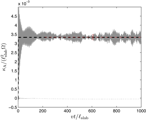
Figure 2. Raw data (gray area) and time average (red dashed line with error bar) of the drift coefficient κA in slab turbulence. The black dashed line shows the classical scattering result from Equation (13), whereas the black dotted line confirms that the coefficient <Δx Δy > /2t is approximately zero, as expected.
Download figure:
Standard image High-resolution image
Figure 3. Raw data (gray area) and time average (red dashed line with error bar) of the drift coefficients κA in 2D turbulence (panel (a)), composite turbulence with 15% slab and 85% 2D (panel (b)), and isotropic turbulence (panel (c)). In all panels, the black dashed line shows the classical scattering result from Equation (13).
Download figure:
Standard image High-resolution imageFor the unperturbed orbit—which, in the case of a homogeneous magnetic field and vanishing electric fields, is a spiral trajectory—the drift coefficient can be evaluated analytically (Minnie et al. 2007; Shalchi 2011). The exact result is
which illustrates that, unlike any macroscopic drift velocity, the drift coefficient does not require the presence of turbulence or of gradients in the mean magnetic field.
In Figure 1, simulation results for the drift coefficient in slab turbulence are shown for early times t ⩽ 10ℓslab/v in comparison to the unperturbed result. So long as parallel scattering is not important, the unperturbed result is retained, whereas for later times the transition to the late-time result is exhibited. Moreover, it is important to note that Figure 1 illustrates the collective behavior of all particles and not an individual particle trajectory. The relatively large fluctuations in the drift coefficients can be understood by using the analogy of beat tones in acoustics. Since all particles have the same rigidity, their (unperturbed) gyrofrequency will to some extent determine the velocity components entering Equation (12).
In Figure 2, the slab drift coefficient is shown for late times, illustrating the agreement with the classical scattering result from Equation (13). Furthermore, both Figures 1 and 2 demonstrate that the symmetric off-diagonal element, <Δx Δy > /(2t), is zero as expected from the remarks in Section 2.1. Furthermore, Figure 3 shows the drift coefficients for the remaining cases of 2D turbulence, composite turbulence7 with 15% slab and 85% 2D, and isotropic turbulence.
The overall conclusion is that, for low turbulence strengths, the weak scattering result κWSA = vRL/3 can be confirmed with good accuracy. The geometry of the fluctuating magnetic field only plays a role insofar as 2D turbulence seem to cause a higher fluctuation in the drift coefficient, whereas slab and isotropic turbulence result in a relatively smooth drift coefficient.
3.2. Results for Strong Turbulence
In Figure 4, the drift coefficient κA is shown as a function of the average turbulence strength normalized to the background magnetic field magnitude, i.e., δBslab/B0. A slab turbulence geometry is assumed and the particle velocity is chosen so that RL = 0.1ℓslab.
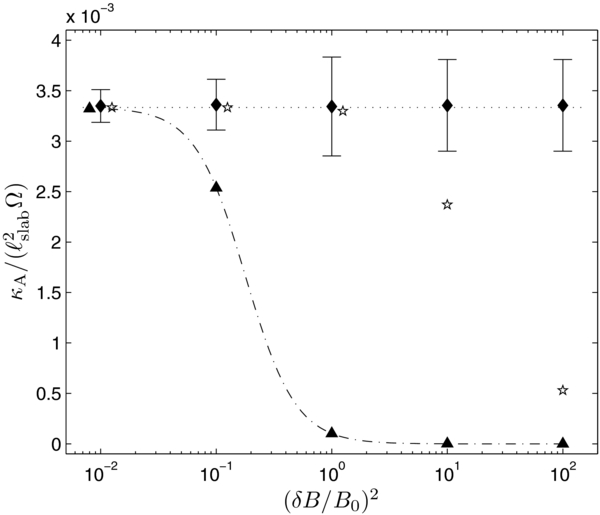
Figure 4. Time-averaged simulated drift coefficient κA (diamonds with error bars) in slab turbulence for different values of the turbulent magnetic field strength, δBslab, normalized to the background magnetic field, B0. The dotted line denotes the weak scattering limit from Equation (7), whereas the stars illustrate the classical scattering result from Equation (13). Furthermore, the BAM model from Equation (14) is shown (dot-dashed line with triangles), which underestimates the drift coefficient for intermediate turbulence levels.
Download figure:
Standard image High-resolution imageFirst one notes that, as a function of time, the drift coefficient κA exhibits stronger fluctuations as the relative turbulence strength, δBslab, is increased. The time-averaged mean value, however, remains in excellent agreement with the weak scattering limit from Equation (7). Moreover, it is shown in Figure 4 that both the classical scattering limit (13) and the BAM formula (14) do not give the correct value for the drift coefficient. The only exception is found at the lowest turbulence strength where λ∥ ≫ RL so that the Equation (13) approximately agrees with the weak scattering limit.
In Figure 5, the drift coefficient κA is shown for isotropic turbulence. For varying turbulent magnetic field strength, the best fit gives
with a = 0.42 ± 0.03 and b = 1.35 ± 0.09. Note that, despite the relatively large errors in the values for the drift coefficient, the results are only qualitatively compatible with a similar formula by Candia et al. (2002), who found a = 0.05 and b = 1.5. In general, Equation (18) describes a reduction of the drift coefficient at smaller turbulence levels than predicted by the classical scattering result, which is also shown for comparison. In the literature, this behavior has been named suppression.

Figure 5. Same as Figure 4, only that now isotropic turbulence is assumed. The dashed line illustrates the best fit from Equation (18). Furthermore, the dot-dashed line shows the result from Candia & Roulet (2004).
Download figure:
Standard image High-resolution imageIn Figure 6, the drift coefficient κA is shown for composite turbulence7 with 15% slab and 85% 2D. For the best fit in Equation (18), the parameters are now a = 1.09 ± 0.52 and b = 0.81 ± 0.35. Furthermore, the classical scattering result from Equation (13) is shown, illustrating that (with the example of the last data point, which, in view of the other results, must be seen as a coincidence) it predicts too large values for the drift coefficient. The comparison with the BAM model from Equation (14) shows that the drift coefficient is underestimated for strong turbulence, in contrast to the classical scattering result from Equation (13), which overestimates κA.
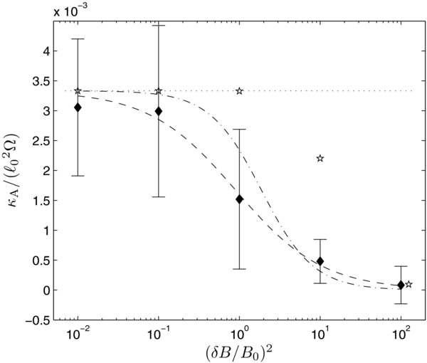
Figure 6. Same as Figure 4, only that now composite turbulence is assumed with 15% slab and 85% 2D. The dashed line illustrates the best fit from Equation (18). For comparison, the dot-dashed line repeats the result for isotropic turbulence (Figure 5).
Download figure:
Standard image High-resolution imageAdditionally, one could ask whether there is a rigidity dependence of the deviation between the simulated drift coefficient and the weak scattering result. Figure 7 illustrates that, for the case of isotropic turbulence with a relative strength δB = B0, such a relation exists but it is weak. However, the tendency shows that, for more energetic particles, the deviation of the drift coefficient from the weak scattering result becomes less pronounced.

Figure 7. Illustration of the weak dependence of the simulated drift coefficient κA normalized to the weak scattering result (diamonds with error bars) from the particle rigidity, RL/ℓ0. Shown is the case of isotropic turbulence with δB = B0. For comparison, the dotted line illustrates weak scattering result from Equation (7).
Download figure:
Standard image High-resolution image3.3. Non-constant Energy Range
A key parameter in the theory of wandering magnetic field lines and perpendicular diffusion of energetic particles is the energy range spectral index q, which describes the behavior of turbulence at largest scales (see, e.g., Shalchi & Weinhorst 2009, and references therein). Therefore, it is an interesting task to explore the influence of the parameter q on the drift coefficient.
In Figure 8, the drift coefficient κA is shown for a varying energy range spectral index of the turbulence power spectrum, i.e., for different values of q in Equation (16). Again, pure slab turbulence has been used with a relative strength of δBslab/B0 = 0.1 and the particle rigidity is RL = 0.1ℓslab. A series of simulations has been performed for q = −0.5, q = 0, q = 0.5, and q = 1. All our results are in excellent agreement with the weak scattering limit from Equation (7) (dashed line).
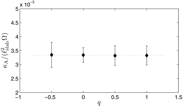
Figure 8. Time-averaged drift coefficient κA (diamonds with error bars) in slab turbulence with δBslab/B0 = 0.1 for different values of the energy range spectral index q which determines the behavior at large scales—see Equation (16). The dotted line denotes the weak scattering limit from Equation (7).
Download figure:
Standard image High-resolution image3.4. Plasma Wave Effects
In this subsection, it is assumed that the magnetic turbulence is no longer static but instead is composed of Alfvén plasma waves, which have the dispersion relation ω = ±vAk. Here,  denotes the Alfvén velocity with ρ the particle mass density (Schlickeiser 2002). Numerically, the turbulence now consists of a superposition of Alfvén waves instead of (time-independent) standing Fourier modes (e.g., Michałek & Ostrowski 1998; Tautz 2010b).
Using the spectrum from Equation (16) for q = 0, the drift coefficient has been investigated by Stawicki (2005) using plasma wave turbulence. The dominant contribution to the drift coefficient for the case of Alfvénic slab turbulence can be written as
whereupon the drift coefficient becomes independent of the particle rigidity and instead depends solely on the Alfvén velocity. Figure 9 shows the drift coefficient for the cases of Alfvénic slab turbulence with and without a turbulent electric field. Whereas, in the absence of an electric field, the weak scattering result is retained, the drift coefficient is considerably enhanced if the electric field is included, showing that the result is in good agreement with Equation (19).

Figure 9. Raw data (gray area) and time average (red dashed line with error bar) of the simulated drift coefficient κA in Alfvénic slab turbulence without (panel (a)) and with (panel (b)) a turbulent electric field, respectively. The black dashed line shows the weak scattering limit from Equation (7), whereas the green dot-dashed line in panel (b) illustrates the analytical result of Stawicki (2005) from Equation (19).
Download figure:
Standard image High-resolution image
Physically, it can be shown that, for plasma wave turbulence, κA is essentially a result of the δE × B0 drift in agreement with Equation (4), where the perpendicular force results from the electric component of the plasma waves (Stawicki 2005).
4. DISCUSSION AND CONCLUSION
In this paper, the asymmetric component of the diffusion tensor—which, for axisymmetric systems, is represented by a single drift coefficient—has been investigated using numerical Monte Carlo test-particle simulations. Special emphasis was focused on (1) the effect of the turbulence level relative to the mean magnetic field strength, (2) the turbulence geometry as well as the energy range in the turbulence spectrum, and (3) the time dependence of the turbulence, thereby illustrating that turbulent electric fields play an essential role for the drift coefficient.
To our knowledge, there has been no other numerical investigation of the drift coefficient that encompasses the combined effects of (1) all contemporary models for the turbulence geometry, (2) varying energy range spectral index, (3) magnetohydrodynamic plasma wave effects, (4) particle energy, and (5) magnetic turbulence strength.
The main conclusions that were obtained from the comparison of the simulation results to several analytical derivations and approximations are as follows.
- 1.For slab turbulence, the agreement between the simulation results and the weak scattering limit is excellent even in the case of strong turbulence. The BAM model, in contrast, predicts a decreasing drift coefficient for turbulence strengths δB/B0 ≳ 0.1.
- 2.For composite and isotropic turbulence, the simulation results for the drift coefficient are in agreement with the weak scattering limit only in the case of weak turbulence. For intermediate and strong turbulence, the drift coefficient is suppressed in agreement with previous simulation results (e.g., Candia & Roulet 2004; Minnie et al. 2007). The classical scattering result, however, which also predicts a decrease of the drift coefficient for a decreasing parallel mean free path (corresponding to higher turbulence strengths), could not be reproduced.
- 3.The value of the particle rigidity—as expressed through the ratio of the Larmor radius and the turbulence bend-over scale—has a negligible influence on the drift coefficient compared to that of the turbulence strength.
- 4.Only a weak influence could be found of the energy range spectral index q on the drift coefficient. Such is in contrast to, for example, the field line diffusion coefficient, which is dominated by the energy range spectral index (e.g., Shalchi & Kourakis 2007).
- 5.For time-dependent Alfvénic slab turbulence, the weak scattering result is accurate only if the turbulent electric field is neglected. With the inclusion of electric fields, stochastic acceleration processes and E × B drift motions increase the value of the drift coefficient.
The comparison with previous simulations by Candia & Roulet (2004) shows that a lower magnitude of the magnetic turbulence is needed to suppress the drift coefficients. First, the fact that Candia & Roulet used a different numerical technique should have no influence on the results. But the deviation can be understood when taking into account the difference spectra used in the simulations. Whereas Candia & Roulet assumed a pure power-law-type spectrum k−s, therefore effectively neglecting the large-scale structures, we included the small-wavenumber regime by assuming a spectrum with a variable energy range spectral index q. For q ≲ 0 in Equation (16), which corresponds to a turbulence spectrum with a negative slope also in the energy range, perpendicular transport is almost diffusive because the field lines are ballistic (Shalchi & Kourakis 2007). Such results in an additional contribution to the drift coefficient, which could increase the value of κA in the transition regime from small to large turbulence amplitudes—exactly what is exhibited by the previous results.
Future work should investigate the qualitative behavior of the drift coefficient in terms, for example, of the unified nonlinear guiding center theory by Shalchi (2010), which, for the first time, revealed agreement between simulations and analytical theory for the cases of magnetostatic slab and composite turbulence (Tautz & Shalchi 2011). Furthermore, the drift motion resulting from the stochastic electric field of plasma waves has to be investigated in more detail both qualitatively, using analytical theory, and quantitatively, by means of numerical simulations for different wave types and polarization properties.
In view of the application of drift coefficients, e.g., to the cosmic-ray density modulation induced by the solar cycle, the large-scale drift effects that result from the curvature of the mean magnetic field have to be included, for example, using the formalism of adiabatic acceleration. Such will then contribute to a more complete understanding of the relevant parameters that enter diffusion–convection equations.
R.C.T. acknowledges help with the ZAA computing cluster by S. Harfst and U. Bolick. A.S. acknowledges support by the Natural Sciences and Engineering Research Council (NSERC) of Canada.
Footnotes
- 3
- 4
- 5
A similar relation exists for the perpendicular mean free path, i.e., λ⊥ = 3κ⊥/v.
- 6
A reviewer has asked whether or not we have been able to reproduce any of the Giacalone & Jokipii (1999) results. Such is indeed possible if the same normalization for the turbulent magnetic field is chosen. Minor deviations can be explained by a slightly different form of the turbulence spectrum that has been used by Giacalone & Jokipii (1999). A discussion of both agreement and difference of the Padian code to other existing codes including that of Giacalone & Jokipii (1999) as well as a plot of the mean free path values is given in Tautz (2010a, 2011).
- 7
Note that for all simulations with composite turbulence, ℓslab = ℓ2D is assumed.