


ABSTRACT
We investigate the active galactic nucleus (AGN) sub-population of a 24 μm flux-limited galaxy sample in the Spitzer Extragalactic First Look Survey. Using deep Keck optical spectroscopy and a series of emission-line diagnostics, we identify AGN-dominated systems over broad redshift 0 < z < 3.5 and luminosity 9 < log (LTIR) < 14 ranges, with sample means of 〈z〉 = 0.85 and 〈log (LTIR)〉 = 11.5. We find that down to the flux limits of our Spitzer MIPS sample (f24 > 200 μJy), 15%–20% of sources exhibit strong AGN signatures in their optical spectra. At this flux limit, the AGN population accounts for as much as 25%–30% of the integrated 24 μm flux. This corresponds to an MIR AGN contribution ≈2–3 × greater than that found in ISOCAM 15 μm studies that used X-ray AGN identifications. Based on our spectroscopically selected AGN sample, we also investigate the merits of Infrared Array Camera (IRAC) color selection for AGN identification. Our comparison reveals that although there is considerable overlap, a significant fraction of spectroscopic AGNs are not identifiable based on their MIR colors alone. Both the measured completeness and reliability of the IRAC color selections are found to be strongly dependent on the MIR flux limit. Finally, our spectroscopic AGN sample implies as much as a 3 × higher AGN surface density at high redshift (z > 1.2) than that of recent optical surveys at comparable optical flux limits, suggestive of a population of heavily obscured, optical/UV reddened AGNs.
Export citation and abstract BibTeX RIS
1. INTRODUCTION
Cosmological models have demonstrated the feasibility of coeval active galactic nucleus (AGN) and spheroid growth via major mergers of gas-rich galaxies. The physical mechanisms include merger-driven gas inflows that trigger starbursts and black hole accretion, as well as supernova and AGN feedback that subsequently quench both star formation and black hole growth (Barnes 2004; Matteo et al. 2008; Croton et al. 2006; Hopkins et al. 2006, 2008; and references therein). These feedback mechanisms are a key component of the galaxy evolution models that predict observables such as the large population of red, passively evolving old stellar populations at high redshift, quasar luminosity evolution, and clustering and host galaxy properties (e.g., Bell et al. 2004; Hopkins et al. 2008).
From an observational standpoint, a complete census of AGN versus star formation activity and their respective bolometric luminosity evolution will provide an important further constraint on the models. Unfortunately, the compilation of such a census remains elusive due to physical mechanisms ranging from relatively mild reddening effects that bias large optical/UV surveys (Wolf et al. 2003; Croom et al. 2004; Richards et al. 2005; Casey et al. 2008) to severe dust obscuration at the cores of an elusive dust-obscured AGN population predicted by both the unified AGN model (Antonucci 1993; Urry & Padovani 1995) and the observed hard X-ray background (Brandt & Hasinger 2005; Comastri et al. 1995; Madau et al. 1994).
Despite the observational challenges, enormous strides in the development, calibration, and comparison of spectroscopic and photometric AGN selection techniques over wavelengths spanning X-ray and optical through MIR and radio have been made in recent years. Through these efforts it has become increasingly clear that though there is no single diagnostic that will provide a complete census of AGN activity over the full range of luminosities and redshifts, a combination of techniques should allow for the eventual reconstruction of the overall sample. As an example, it has been shown that the local sample can be characterized with optical emission-line diagnostics that not only separate star formation and various AGN-dominated sources (Seyferts versus LINERs), but also quantify relative AGN contributions within the composite population (Kewley et al. 2006; Yuan et al. 2010; Moustakas et al. 2010). Subsets of these optical diagnostics have also been applied to large intermediate redshift samples with great success (Montero-Dorta et al. 2009; Patel et al. 2010; Symeonidis et al. 2010). In more distant populations, our dependence on X-rays (Mushotzky et al. 2000; Alexander et al. 2003; Bauer et al. 2004), which themselves have been shown to be susceptible to extreme obscuration (Brandt & Hasinger 2005; Treister & Urry 2005; Donley et al. 2005; Martínez-Sansigre et al. 2007), has ended. A variety of MIR color (Lacy et al. 2004; Stern et al. 2005) and power-law (Alonso-Herrero et al. 2006; Barmby et al. 2006) selections have been shown to be effective diagnostics when properly applied. Despite some known redshift-dependent limitations regarding their reliability and completeness, Infrared Array Camera (IRAC) color selection (Chary et al. 2004; Barmby et al. 2006; Donley et al. 2008; Georgantopoulos et al. 2008) remains an attractive method for identifying AGNs, particularly for large area surveys for which other approaches become prohibitively costly.
More recently, MIR Spitzer Infrared Spectrometer spectroscopy has been shown to be incredibly effective at not only distinguishing even heavily enshrouded, Compton-thick AGNs from star formation (Polletta et al. 2008; Alexander et al. 2008), but also at quantifying their relative contributions for individual sources (Yan et al. 2007; Farrah et al. 2007; Veilleux et al. 2009; Fadda et al. 2010). Based on the results above, it is becoming increasingly clear that the ultimate census of AGNs in their various incarnations and over a large range of cosmic timescales will rely on a multi-wavelength patchwork of selection techniques (e.g., Sajina et al. 2008; Park et al. 2008; Kartaltepe et al. 2010).
In this paper, we take the approach of pre-selecting a flux-limited 24 μm sample and using deep spectroscopic follow-up observations to search for AGN signatures. We utilize a range of AGN-line diagnostics to achieve broad redshift coverage. Spectroscopic AGN identification has the advantage that emission-line diagnostics tend to be less impacted by reddening than broadband color selection or even spectral energy distribution (SED) fitting techniques. In many cases, the identification of a single high-excitation line or broad-line profile is sufficient to identify an AGN ionization source. Because line ratios are normalized to the continuum, they tend to be more robust to reddening than broadband colors. This approach is by no means impervious to attenuation effects, since the most heavily obscured populations have faint or no optical counterparts. Even in these cases, however, it is often possible to identify AGN emission lines in continuum-less spectra. Based on this spectroscopic 24 μm sample, we investigate the effectiveness of emission-line diagnostic and mid-infrared color selection. We then use our AGN sample to directly quantify the AGN component of MIR source counts and investigate the population of high-redshift luminous AGNs that may be missing from optical/UV-selected samples.
This paper is divided into the following sections. A summary of the various observational components and their basic analysis is given in Section 2. A description of our AGN identification and a comparison to IRAC color-selected samples is given in Section 3. Infrared luminosities and the total IR AGN contribution are computed in Section 4. Finally, a comparison to optical quasar samples is discussed in Section 5. The main points of this work are summarized in Section 6. Throughout the paper, we adopt the cosmology of Ωm = 0.27,  and H○ = 70 km s−1 Mpc−1. We also adopt the Vega system for all optical R-band magnitudes.
2. SAMPLE AND OBSERVATIONS
The Spitzer Extragalactic First Look Survey (FLS)5 region is a ≈4 deg2 region chosen to lie within the continuous viewing zone, having minimum cirrus and no bright radio sources. It is centered around R.A. = 17h18m00s, decl. = 59°30'00''. The extragalactic component of the FLS is comprised of IRAC (Fazio et al. 2004) 3.6, 4.5, 5.8, and 8.0 μm and Multiband Imaging Photometer for Spitzer (MIPS; Rieke et al. 2004) 24, 70, and 160 μm observations taken in 2003 December with a total exposure time of 63 hr. In addition to IR imaging, numerous ancillary data sets including radio, optical and near-IR (NIR) data have been taken in this field. The primary data sets used for this study, MIPS 24 μm imaging and Keck optical spectroscopy, are described below. Details about the IRAC and optical photometry that are incorporated into this work can be found in Lacy et al. (2005), Fadda et al. (2004), and Shim et al. (2006).
2.1. Spitzer MIPS 24 μm Selected Sample
The MIPS 24 μm areal coverage is 4.4 deg2 for the main field and 0.26 deg2 in a deeper verification field, with respective 3σ depths of 0.11/0.08 mJy (Fadda et al. 2006). All data were processed and stacked by the data processing pipeline at the Spitzer Science Center. MIPS photometry was performed using APEX, the Spitzer Astronomical Point Source EXtraction package, which performs point-response function (PRF) fitting for source extraction. A complete description of the 24 μm data reduction and source catalog can be found in Fadda et al. (2006).
A 24 μm flux-limited subsample of 337 sources with f24 > 200 μJy was targeted for spectroscopic follow-up (〈f24〉 = 400 μJy). Sources with f24 > 800 μJy, which account for 15% of the sample, were given highest priority in our selection, producing a slight bias toward luminous sources. We find that due to the relatively low surface density of these bright sources, the impact on our overall sample is small. Nonetheless, it is accounted for in our analysis with the adoption of a simple single-step selection function that will be described in Section 4.2.
2.2. Optical Spectroscopy
Optical spectroscopy was obtained with the Deep Imaging Multi-Object Spectrograph (DEIMOS; Faber et al. 2003) on the W. M. Keck II 10 m telescope over two nights from UT 2005 June 7–8. A 600 line mm−1 grating with a central wavelength setting of 7300 Å and a GG455 blocking filter produced spectra with a 0.65 Å pix−1 mean spectral dispersion and a total spectral coverage of 5300 Å.
Our spectroscopic sample is distributed over six 5' × 16 3 slitmasks that sample a non-contiguous ≈500 arcmin2 region of the FLS. In a typical mask, ≈100 slits were observed, roughly half of which make up our primary sample. Slitmask observing information is listed in Table 1, and for illustration, their positions are overlaid on a MIPS 24 μm image in Figure 1.
Figure 1. MIPS 24 μm image of the full 2 0 × 25 region of the FLS Verification region. Positions of six 5' × 17' Keck DEIMOS optical spectroscopy slitmasks are shown. A summary of the spectroscopic observations is given in Table 1.
Download figure:
Standard image High-resolution imageTable 1. Spectroscopic Observation Log
| ID | R.A. (J2000) | Decl. (J2000) | P.A. (deg) | Exp. Time (ks) |
|---|---|---|---|---|
| M1 | 17:12:32 | +58:47:52 | 140 | 2.7 |
| M2 | 17:23:17 | +59:08:09 | 160 | 3.6 |
| M3 | 17:15:15 | +60:12:19 | 0 | 2.9 |
| M4 | 17:17:05 | +60:17:53 | 124 | 2.3 |
| M5 | 17:22:02 | +58:49:06 | 155 | 3.6 |
| M6 | 17:20:40 | +59:12:17 | 140 | 3.0 |
Download table as: ASCIITypeset image
Source selection is based purely on the 24 μm flux; however, optical or NIR astrometry is adopted when available. To produce our band-merged source list, the MIPS catalog was matched independently to the IRAC 3.6 μm and R-band catalogs using a simple nearest neighbor matching algorithm with a 2'' search radius. The chosen search radius is based on an analysis of the distribution of astrometric separations between the different catalogs. For instance, the 1σ positional uncertainty for MIPS-to-optically matched sources, as well as the MIPS-to-IRAC sources is 0 6, consistent with the positional uncertainty of the MIPS catalog. At the depths of our optical and IRAC catalogs, we determined that with a 2'' search radius the probability of spurious matches is negligible.
Based on the band-merging approach described above, optical counterparts were identified for 80% of the MIPS targets; IRAC-only counterparts were identified for another 15%, and MIPS-only targets with no identifiable optical or IRAC counterpart accounted for the remaining 5% of the targets. For the slitmask design, no priority was given based on the detection of counterparts, so a MIPS-only source is just as likely to be targeted as one with an optical and IRAC counterpart. When detected in multiple bands (i.e., R and/or IRAC 3.6 μm ), the shortest wavelength data set was used for slit position refinement. Finally, we use 1'' wide slits tilted 10° from the spatial axis and require a minimum projected slit length of 7''. This results in a mean spectral resolution of 3.5 Å FWHM.
Total integration times for the six masks ranged from 2.3 to 3.6 ks, divided into multiple exposures. Typical observing conditions were ≈07 FWHM (R band), but varied from ≈05 to 10 FWHM. For the initial data reduction, we use the DEEP2 spec2d pipeline,6 which is based on the Sloan Digital Sky Survey (SDSS) spectral reduction package. This package performs cosmic ray removal, flat-fielding, co-addition, sky subtraction, wavelength calibration, and both two-dimensional and one-dimensional spectral extraction.
In Figure 2, redshift versus R-band magnitude is shown for the 24 μm spectroscopic sample. After the exclusion of 18 corrupt or contaminated slits and 14 spectroscopically confirmed stars, we were left with a sample of 305 sources for which spectra were obtained. Of these, 212 were determined to have high-quality spectroscopic redshifts in the range 0 < z < 3.4 and with a sample mean of 〈z〉 = 0.85. The remaining 93 sources have ambiguous or no redshift determinations and in many cases exhibit no measurable continuum. Excluding the stellar sources and corrupt sources, this translates to a 70% spectroscopic efficiency for our 24 μm selected, extragalactic sample. The overplotted redshift efficiency histogram clearly shows that our redshift efficiency exhibits a strong optical magnitude dependence. Brighter than R < 24 mag, our sample is 88% complete.
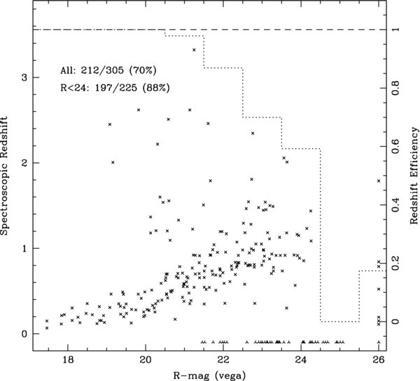
Figure 2. Spectroscopic redshift vs. R-band magnitude for our 24 μm selected sample. High-confidence redshifts are obtained for 212/305 (70%) of the targeted sample (crosses). Sources with no or poor-quality spectroscopic redshifts are assigned the redshift z = −0.1 (three-point stars). An overlaid histogram shows our spectroscopic redshift efficiency (scale shown on the right axis). Integration of this histogram shows that we are 88% complete down to R < 24.0.
Download figure:
Standard image High-resolution image2.3. Emission-line Measurements and Redshift Identification
The one-dimensional spectral output of the DEEP2 pipeline is analyzed using an in-house IDL package written by PIC and DF. Galaxy redshifts are identified through visual inspection and galaxy template cross correlation. Line flux, equivalent width, and kinematic measurements are made by performing Gaussian profile fits to the one-dimensional spectra. This is done interactively with the user identifying the lines to be fit and specifying the spectral region over which to perform the line+continuum fit. Most lines are fit individually, but in the case of the Balmer lines, two-component emission+absorption profiles are adopted. It is well known that nebular Balmer emission lines can suffer from contamination due to underlying stellar absorption and subsequently be underestimated. In terms of AGN classification, this would artificially boost line ratio diagnostics that rely on Balmer lines, most notably [O iii]/Hβ. Our high spectral resolution enables us to resolve and directly measure the nebular emission and the pressure broadened stellar absorption components, eliminating the need for a global correction.
3. AGN IDENTIFICATION
We rely primarily on optical spectroscopy for AGN classification. There is no single line diagnostic that will isolate both narrow and broad-line AGNs over the broad redshift range of our sample. Therefore, we adopt the following four emission-line diagnostics with overlapping redshift sensitivities: (1) [N ii]/Hα versus [O iii]/Hβ (classic BPT diagram), (2) [O iii]/Hβ, (3) [Ne v] strength, (4) and the FWHM of strong permitted lines. Example spectra of these classifications are shown in Figure 3.
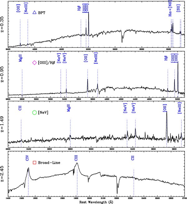
Figure 3. Keck DEIMOS spectra of representative AGNs in our sample. Spanning the redshift range 0.35 < z < 2.45, these spectra provide examples for our four different AGN diagnostics. Top to bottom: (1) a low-redshift (z = 0.35) AGN identified by its strong [N ii]/Hα vs. [O iii]/Hβ line ratios (BPT), (2) an intermediate redshift (z = 0.95) AGN with log([O iii]/Hβ) >0.9, (3) a z = 1.49 AGN with strong [Ne v] emission, and (4) a z = 2.45 broad-line AGN. Throughout this paper, these selection criteria are associated with the open symbols: triangle, diamond, circle, and square, respectively.
Download figure:
Standard image High-resolution imageThe first three diagnostics are sensitive to a redshift of z ≲ 1.5. The last is essentially uniformly sensitive to the limits of our survey. At low redshift (z < 0.5), the classic emission-line ratio plot of [N ii]/Hα versus [O iii]/Hβ separates AGN-dominated and starburst-dominated galaxies (Baldwin et al. 1981; Veilleux & Osterbrock 1987; Kauffmann et al. 2003; Kewley et al. 2006). In Figure 4, we show this plot for all sources with well-measured emission-line ratios along with the demarcation lines of both Kauffmann et al. (2003), who derive an empirical separation based on the SDSS sample and Kewley et al. (2001), who use theoretical models and derive a more conservative separation. The intermediate region between the two has been shown to be dominated by transition sources (Kewley et al. 2006), and since our primary interest is to identify AGN-dominated systems, we adopt the conservative approach of only including candidates above the more stringent Kewley extreme starburst demarcation line. Based on this selection, we find that three of 40 low-z sources are AGN-dominated, falling in the Seyfert/LINER region of the plot. Note that we only use this diagnostic to separate AGNs from transition and star-forming objects and make no attempt to further separate LINERs and Seyferts.
At intermediate redshifts (0.4 ≲ z ≲ 1.0), neither Hα nor [N ii] is accessible in the optical; however, the [O iii]/Hβ ratio can still be used. For sources with only this ratio available, we adopt a limiting value of log([O iii]/Hβ) > 0.9. Comparison to Figure 4 shows that this is a conservative limit that sacrifices completeness for reliability. Adopting this criteria, we find that six sources for which this ratio is accessible are clearly AGNs.
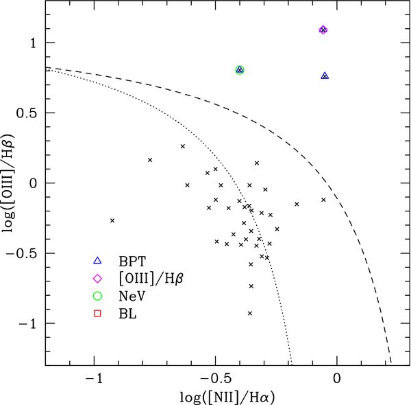
Figure 4. AGN-line diagnostic plot [O iii]/Hβ vs. [N ii]/Hα for a low-redshift subset (N = 40) for which both line ratios are well determined. The AGN–starburst demarcation curves of Kewley et al. (2001) and Kauffmann et al. (2003) are shown as dashed and dotted lines. Based on these diagnostics, we find that 3 of the 40 sources are unambiguously identified as AGNs (open symbols). An additional 11 sources satisfy the Kauffmann et al. (2003) criteria. By following the classification of Kewley et al. (2006), we adopt these as transition objects and exclude them from our AGN-dominated sample. Open symbols are overplotted on spectroscopically identified AGNs and are the same as in Figure 3.
Download figure:
Standard image High-resolution imageAt high redshift (z ≳ 0.9), where none of these line ratios are optically accessible, we rely on the presence of the high-excitation [Ne v] λ3426 forbidden lines. We find 18 sources with strong [Ne v] emission indicative of a dominant AGN. This population has a median redshift of z ∼ 1.
Finally, over the entire redshift range, we are sensitive to the detection of various broad permitted lines, including Balmer lines, Mg ii, C ii, C iii, C iv, and Lyα. In Figure 5, the maximum FWHM for all measured permitted emission lines is shown as a function of redshift. Broad-line AGNs are typically identified based on line widths in excess of 800–2000 km s−1. Based on the velocitymax distribution of our sample, we adopt a minimum line width of 2000 km s−1 and identify 23 of 212 sources that meet this criteria.
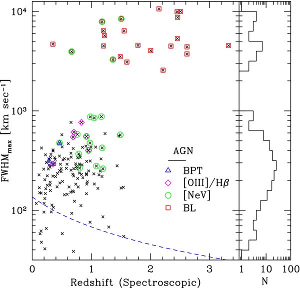
Figure 5. Emission-line FWHMmax vs. spectroscopic redshift. The FWHMmax is defined as the FWHM of the broadest measured emission line in a given galaxy's optical spectrum. Sources with FWHMmax > 2000 km s−1 are identified as broad-line AGNs. Open symbols are overplotted on spectroscopically identified AGNs and are the same as in Figure 3. Dashed line represents the spectral resolution limits of our data.
Download figure:
Standard image High-resolution image3.1. Comparison to IRAC Color Selection
Numerous independent efforts have attempted to utilize Spitzer IRAC colors to create an AGN diagnostic that is invariant to dust obscuration. We use our spectroscopically selected AGN sample to investigate the completeness and reliability of two of these MIR color selection techniques (Lacy et al. 2004; Stern et al. 2005, hereafter L04 & S05). In Figure 6, we show the MIR log (f8.0/f4.5) versus log (f5.8/f3.6) and log (f3.6/f4.5) versus log (f5.8/f8.0) color–color distributions for all sources in our spectroscopically targeted sample with four-channels IRAC detections. The distribution of our AGN sample in IRAC color space shows a good general correspondence between our spectroscopically identified AGNs and the AGN regions of color–color space defined by L04 and S05.
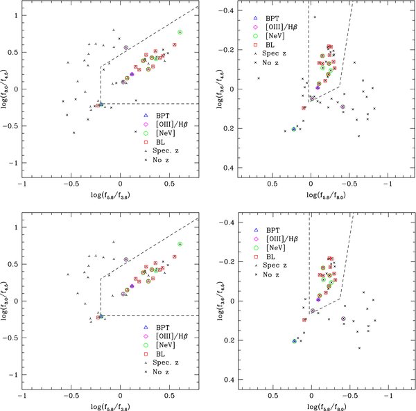
Figure 6. IRAC four-channel color–color plots for sources with measured four-color photometry (top) and a subset of the sample at the bright end of our IRAC flux distribution (bottom). Sources with and without spectroscopic redshift are shown as four-point and three-point stars, respectively. Open symbols are overplotted on spectroscopically identified AGNs and are the same as in Figure 3. The AGN regions defined by L04 (left) and S05 (right) are marked by dashed lines. Top panels: down to the IRAC flux limit of the Spitzer Extragalactic First Look verification survey, the L04 and S05 IRAC color criteria identify 70% and 50% of the spectroscopic AGNs, respectively. Conversely, of the sources in the IRAC-selected AGN regions, 50% and 60% are spectroscopically confirmed. Bottom panels: at the bright end of the IRAC flux distribution, the IRAC color selections are considerably more effective in terms of both completeness and reliability—80% and 70%, respectively for the L04 selection and 80% and 80% for the S05 selection.
Download figure:
Standard image High-resolution imageThe spectroscopic AGN fraction is seen to be 3–4 × higher inside these regions than outside, based on either of the two IRAC color criteria. This correspondence suggests that the IRAC color selection is a statistically efficient way of targeting AGN candidates. In terms of completeness of the IRAC selection criteria, we find that 70% and 50% of the spectroscopically identified AGNs are found in the L04 and S05 defined AGN regions, respectively. When restricted to broad-line systems, these percentages increase to 90% and 70%. Alternatively, if we make the extreme assumption that all of the IRAC color selected AGNs are missing from our selection due to heavy obscuration, the respective completeness fractions rise to 80% and 70%.
With respect to the reliability of IRAC selection, we find that 50% and 60% of sources found in the L04 and S05 IRAC AGN regions are spectroscopically confirmed AGNs. Though these fractions may appear low at first glance, it is also worth emphasizing that the quoted reliabilities above are only lower limits for the flux range of our sample. In both the L04 and S05 samples, as many as 1/3 to 2/3 of the IRAC AGNs without spectroscopic confirmation are spectroscopically unidentified. If we were to remove these sources from the calculation, the reliability percentages increase to 60% and 80%. Finally, if we make the assumption that all of the spectroscopically unidentified sources are in fact heavily obscured AGNs the reliability of the IRAC AGN criteria climbs to 70% and 80%. Not surprisingly, the two IRAC selections are fairly comparable down to flux limits of our sample (f24 > 200 μJy). The primary difference being that the S05 color selection casts a slightly more conservative net that produces a less complete, but more reliable AGN sample.
The values quoted above are notably lower than those of S05 who, using a larger, but shallower AGES spectroscopic sample (R < 21.5), find that both their completeness and reliability is ∼80%. A direct comparison between the samples is impossible given the differences in selection criteria of our samples. It is not clear how our 24 μm sample, which is biased toward AGN and star-forming systems, should compare to the optical+IRAC+X-ray selection of the sample used in S05. We initially suspected that the increased depth of our spectroscopic survey might be responsible; however, we found that restricting our sample to the AGES magnitude limit made no appreciable impact on the completeness fraction.
The FLS verification depth on which our sample is based is roughly 2× deeper than that of the AGES sample, so another possibility is that the measured completeness and reliability are strongly dependent on the IRAC flux limit. An increased contamination fraction would be consistent with previous findings that at fainter flux levels, MIR color selection picks up high-redshift LIRG populations (Chary et al. 2004; Barmby et al. 2006; Donley et al. 2008; Georgantopoulos et al. 2008). The decreased completeness is not as easily understood, but we investigate both effects by applying the 5σ flux limits of the IRAC shallow survey to our sample, 12.3, 15.4, 76, and 76 μJy at 3.6, 4.5, 5.8, and 8.0 μm, respectively. Application of this simple-minded flux cut pushes the completeness from 50% to 80% and the reliability from 60% to 80% perfectly consistent with the S05 claims of 80% completeness and 20% contamination. The degree of agreement is likely to be a bit coincidental given the significant differences in the spectroscopic selection effects; however, this test clearly reveals the strong flux dependence on both the reliability, as noted in previous works, as well as the completeness of the MIR color selection technique. For the remainder of this paper, we define our AGN sample based solely on our spectroscopic classifications.
4. 24 μm AGN CONTRIBUTION
4.1. Computing IR Luminosities
The extrapolation of MIR luminosities to a total infrared luminosity can have large uncertainties due in part to SED variations from galaxy-to-galaxy and also due to the variations in the rest-frame to observed-frame 24 μm luminosity ratio as a function of redshift, particularly as one moves to high redshift (Dale et al. 2005). The large intrinsic uncertainties associated with the MIR "k-correction" make it difficult to place tight constraints on LTIR. These uncertainties could be further constrained with 70 μm and 160 μm observations; however, for high-redshift samples and at the depths of our sample, those observations can be prohibitively difficult to obtain. Recognizing the large intrinsic uncertainties in extrapolating LTIR from f24 observations, even with known redshifts, we take a simple approach in computing LTIR and then use model SEDs to estimate our uncertainties.
We combine photometry, spectroscopic redshifts, and a suite of model and empirical SEDs to estimate IR luminosities for our sample. For each source with known redshift, we compute LTIR with a range of templates that include: (1) the Dale & Helou (2002) family of model SEDs adopting the approach of Choi et al. (2006), (2) the ensemble of 14 average template SEDs constructed by Rieke et al. (2009, hereafter R09), and (3) a set of purely empirical SEDs: M82, Arp220, PG1613, and Markarian 231. The constructed SED templates span the range of normal through ULIRG galaxies while the empirical SEDs are included to extend the sample to include sources with AGN contribution.
Numerous authors have quantitatively investigated the differences between popular SED templates (Rieke et al. 2009; Goto et al. 2010; Boquien et al. 2010; Elbaz et al. 2010). Most relevant to this effort, R09 offers an analysis of their templates compared to those of Dale & Helou (2002) and Chary & Elbaz (2001). We would not rehash that discussion here except to point out that the R09 templates target a larger luminosity range than either of the other sets, so naturally they produce a larger range of LTIR. Our focus here is a comparison between the R09 templates and our empirical SEDs. We compute LTIR based on their average templates by converting our spectroscopic redshifts into luminosity distances, computing rest-frame 24 μm luminosities based on each of the 14 average templates, and finally computing the LTIR based on their Equation (A6). For the empirical models, we split our sample based on the spectroscopic AGN criteria described in Section 3, and then adopt either a mean M82+Arp220 template or a PG1613+Markarian 231 template. In Figure 7, total IR luminosities based on our empirical SEDs are shown in comparison to those of the R09 templates. In the top panel, the LTIR values computed for the empirical templates (diamonds and stars) are shown in comparison to the envelope of the R09 family of templates, represented by the two extreme templates (triangles). The quantities are shown as a function of LTIR of the median Rieke template, plotted on the abscissa. In the bottom panels, residuals are shown as a function of luminosity and spectroscopic redshift. The extrapolation of LTIR shows its strong redshift dependence, which is a consequence of the fact that the MIPS 24 μm band samples strong polycyclic aromatic hydrocarbon and silicate absorption features over the redshift range of our sample. The uncertainty due to galaxy-to-galaxy variations hits a maximum at redshifts z ≈ 1.4 where the 9.8 μm silicate absorption feature is being sampled, and a minimum at z ≈ 0.6, where the relatively featureless 15 μm region of the MIR SED is being probed.
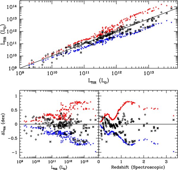
Figure 7. Comparison of our adopted total infrared luminosity (LTIR) to those based on the SEDs of Rieke et al. (2009). Top panel: LTIR based on our empirical SEDs for all sources with measured spectroscopic redshift are plotted against LTIR computed using a R09 median template. Star-forming and AGN-dominated galaxies are shown as diamonds and stars, respectively. The extreme model SEDs from R09 (triangles) represent the full range of LTIR that are consistent with their templates. Intermediate SEDs are excluded for clarity. Bottom panel: LTIR residuals, after subtraction of the median model, as a function of LTIR (left) and spectroscopic redshift (right). Overall, our LTIR estimates are consistent with those of the median R09 template, with particularly good agreement in the LIRG (1010 < LTIR < 1011) range. As one would expect, AGNs tend to trace out the lower edge of the envelope of SEDs, but over our redshift range are only ≈0.3 dex less luminous than the median. Only at low luminosity (LTIR < 1010) do significant inconsistencies arise.
Download figure:
Standard image High-resolution imageOur computed IR luminosities are shown in Figure 8 as functions of redshift and 24 μm flux. It is worth noting that in estimating the total infrared luminosity, different authors use different wavelength ranges as proxies for LTIR, including 3–1100 μm (Dale et al. 2007), 5–1000 (R09), 8–1000 (Sanders & Mirabel 1996; Chary & Elbaz 2001), and 0–∞ (Draine & Li 2007). In this paper, we adopt the 3–1100 μm for both the Dale & Helou (2002) and the empirical templates and the 5–1000 μm range for the R09 templates. The differences between the wavelength ranges are small compared to those due to the range of SEDs (Choi et al. 2006; Boquien et al. 2010), so for the remainder of this paper, we will refer to both estimates as LTIR.
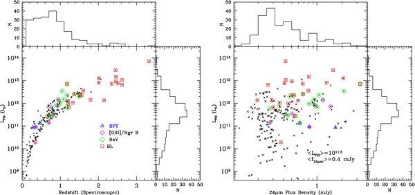
Figure 8. Total infrared luminosity (LTIR) vs. redshift (left) and 24 μm flux (right) plotted for the subsample with high-confidence redshifts. Open symbols are overplotted on spectroscopically identified AGNs and are the same as in Figure 3.
Download figure:
Standard image High-resolution image4.2. AGN Fraction
After removal of stars, the final spectroscopic AGN sample accounts for 20% (42/212) of our spectroscopic redshift sample and 14% (42/305) of our targeted sample. This fraction is expected to be flux dependent, so we determine the AGN 24 μm contribution as a function of MIR flux by applying a step-function correction that accounts for our non-uniform sampling of the 24 μm distribution, as mentioned in Section 2.1. This correction is computed based on a comparison to the 24 μm counts over the full FLS. Our spectroscopically targeted sample is 2.1 × overdense in the 0.8 mJy <f24 < 2.5 mJy flux range relative to the 0.2 mJy <f24 < 0.8 mJy range. This overdense population represents ≈7% of our entire sample and has only a marginal impact on the overall AGN counts; however, uncorrected, it can make a significant flux contribution.
In the top panel of Figure 9, the differential distribution of 24 μm intensity, I24 μm (Jy sr−1), as a function of source flux density, f24, is shown for the targeted sample (N = 305), the redshift sample (N = 212), and the AGN sample (N = 42), all normalized to the full field FLS. Comparison to the full field distribution suggests that our targeted sample does not deviate significantly from the background counts over the 0.2 mJy <f24 < 2.5 mJy flux range. In the bottom panel, the cumulative distribution of the AGN contribution to the I24 μm is shown based on spectroscopically confirmed sources only (solid line).
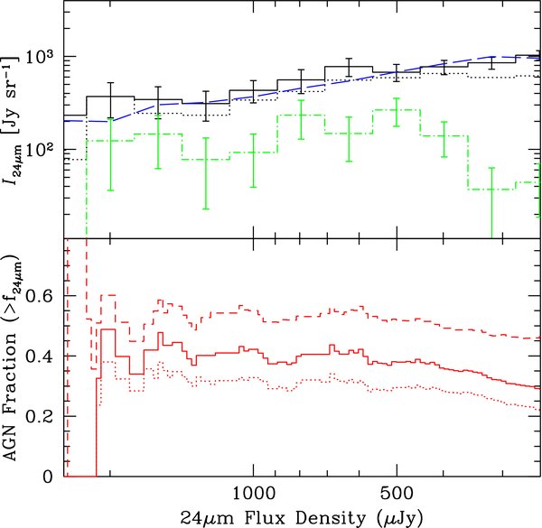
Figure 9. Top panel: the differential distribution of 24 μm intensity, I24 μm, as a function of source flux density for our targeted (solid), spectroscopic redshift (dotted), and AGN (dot-dashed) samples, along with the full-field FLS sample (long-dashed) for comparison. The distribution of our target sample is consistent with that of the full-field FLS sample, suggesting that it is free of any additional f24 selection biases. Bottom panel: the cumulative distribution of the AGN contribution to I24 μm based on the spectroscopically confirmed sample only (solid). Lower and upper limits on the cumulative distributions based on extreme assumptions about non-detections are shown for reference (dotted and dashed, respectively).
Download figure:
Standard image High-resolution imageWe estimate the potential bias due to spectroscopic incompleteness by also including two distributions based on the extreme assumptions that all sources without redshift identification are (1) z > 1.5 star-forming galaxies (dotted line) and (2) spectrally featureless, heavily obscured AGN (dashed line). Even with the adoption of the former conservative assumption, over the 0.3 mJy <f24 < 2.5 mJy range, the cumulative AGN flux contribution is found to be 25%.
In comparison to previous measurements, we find that the AGN contribution to the total 24 μm flux is considerably larger than estimates derived from the X-ray. For instance, in the flux interval 0.5 mJy <f24 < 2.5 mJy, we find a 24 μm AGN flux contribution of 30%–40%, which is 2–3 × higher than the 14.6% found by Fadda et al. (2002) over the 0.5 mJy <f15 < 3.0 mJy range in the Lockman Hole.
A comparison to X-ray selected AGN samples based on Spitzer data shows similar results. In Figure 10, our AGN fraction is compared to that of an X-ray selected sample of Treister et al. (2006) and an X-ray/MIR/Radio sample of Donley et al. (2008). At the brightest 24 μm flux levels we are in good agreement with Treister et al. (2006); however, at fainter fluxes, our corrected fractions are ≈2 × higher, and more in line with the "corrected" sample of Donley et al. (2008).
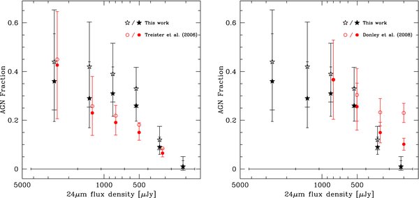
Figure 10. AGN fraction as a function of f24 flux density. In both panels, the AGN fraction based on our spectroscopically selected sample is shown before and after a correction for spectroscopic incompleteness solid vs. open stars. The X-ray selected sample of Treister et al. (2006) and X-ray/MIR/radio sample of Donley et al. (2008) are overplotted in the left and right panels, respectively. In both cases solid and open circles represent the X-ray selected AGN fraction before and after correction for sources that may have been missed in the X-ray sample. Vertical 1σ Poisson error bars are shown. For clarity vertical error bars are left off of our corrected sample as well as that of Treister et al. (2006). The various ratios are computed for the same flux bins, which are shown at the bottom of each panel, but slight artificial vertical offsets are applied to visually separate the samples.
Download figure:
Standard image High-resolution image5. AGN SURFACE DENSITY
The AGN fraction measured above is nearly a factor of two larger than previous measurements based on X-ray AGN identification. Unfortunately, since we lack X-ray coverage in this area, we cannot directly reconcile this discrepancy. Indirectly, we can investigate whether our selection is identifying a unique AGN population missing from previous surveys.
Our full sample is selected to include all sources with dominant optical AGN signatures (i.e., Seyferts and quasars) without explicit redshift, luminosity, or morphology restrictions. At bright optical fluxes, we are dominated by compact, luminous, broad-lined type-I quasars. A direct surface density comparison with minimal additional restriction should therefore reveal if there are any significant differences between the optically bright end of our AGN sample and various UV/optically selected AGN/quasar surveys such as COMBO-17, SDSS, 2QZ, and 2SLAQ that have probed this regime over large areas.
5.1. COMBO-17
The COMBO-17 AGN sample is selected based on multi-band photometry over 17 relatively narrow bandpasses that span the UV to optical wavelengths (Wolf et al. 2003). The "fuzzy spectroscopy" approach enabled the efficient classification of ≈50,000 sources and hundreds of AGN down to R < 24 mag over an solid angle of ≈1 deg2. A comparison of the bright end of our AGN sample (R < 22 mag) to that of the completeness corrected COMBO-17 AGN sample provides a simple test of sample completeness. For the comparison, we apply redshift constraints to our sample to match the sensitivity function of the COMBO-17, which is known to be incomplete below z < 1.2. No additional luminosity, morphology, or color cuts are applied. In Figure 11, we show the cumulative surface density of this sample as a function of R-band magnitude for two redshift intervals: z > 1.2 and z > 2.2. Not surprisingly, the z > 1.2 constraint removes most extended and low-luminosity sources that would not satisfy a classical quasar definition. Of the 17 AGNs that meet the z > 1.2 and R < 22 magnitude criteria, all have stellar-like profiles based on their SExtractor stellarity parameter (stellarity >0.8).
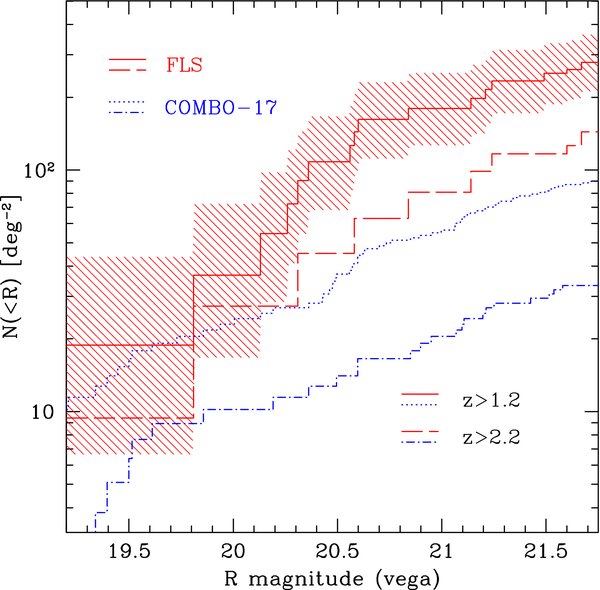
Figure 11. Surface density of spectroscopically identified AGNs as a function of R-band magnitude for subsamples with redshift limits of z > 1.2 (solid) and z > 2.2 (dashed). These redshift cuts allow for the direct comparison to COMBO-17 surface densities (Wolf et al. 2003) over comparable redshift ranges (dotted and dot-dashed). In both redshift ranges, we see that our derived surface densities are ≈3 × higher than those of the COMBO-17 survey. The 1σ confidence interval for the z > 1.2 sample, shown as a hashed region, is based on small number Poisson statistics (Gehrels 1986).
Download figure:
Standard image High-resolution imageThis figure reveals that despite a deficit at bright magnitudes resulting from our relatively small area coverage, by R > 20.5 mag our quasar surface density climbs well above that of COMBO-17 and we measure a ≳ 3 × higher surface density by R < 22 mag. We expected to detect five quasars in our survey area based on the COMBO-17 surface density, so based on simple Poisson statistics, our measured overdensity is significant at the 5σ level.
Given the small size of our sample, some of this overdensity could be attributed to simple cosmic variance. The proper treatment of this issue is beyond the scope of this work; however, the division of our sample into multiple redshift bins in Figure 11 reveals that our sample is not dominated by a single structure. Dividing our sample into low and high-redshift subsamples, we find that the z < 2.2 and z > 2.2 subsamples are both overdense, by factors of 2.6 × and 4.0 ×, respectively. Coupled with the redshift distribution shown in Figure 5, we can rule out the possibility that our elevated counts are due to a single cluster or filamentary structure.
5.1.1. Testing the Significance of the COMBO-17 Overdensity
Above, we assumed a Gaussian spatial distribution to estimate the significance of the measured quasar overdensity. Recognizing that this approach is a poor approximation for non-uniformly sampled clustered populations, we use a Monte Carlo approach to investigate whether our measured overdensity is simply a sampling effect. As discussed in Section 2, our sample is drawn from six non-contiguous regions in the FLS. If the locations of these regions were randomly selected, the summed area of these fields should be representative of the underlying distribution. Unfortunately, since our surveyed field locations were chosen to include luminous 24 μm sources, they are not completely random. This opens the door for two potential biases. The first is due to the primary 24 μm targets themselves contributing to the quasar counts. We can rule out this first scenario based on our spectroscopic data. The optical spectra of this sample confirms that although 10 primary sources were found to have AGN spectral signatures, only 1 of these was above the z > 1.2 redshift cutoff and it was too faint to meet the R < 22 mag limit. Therefore, none of these primary targets directly contribute to the measured quasar overdensity.
The second potential bias is due to the fact that since our fields are centered around bright 24 μm sources, we may be preferentially sampling regions of quasar overdensity. The vast majority of the primary targets with redshifts identification are found to be below the z > 1.2 redshift cutoff (20/23), so this is also not a likely scenario. Nevertheless, we further investigate this possibility below using the publicly released COMBO-17 database of a ≈0.25 deg2 region of the Chandra Deep Field South (CDFS).
To reproduce the uniformly sampled case, we take the full COMBO-17 catalog and draw sources from six randomly located sub-fields sized to match the coverage area of our DEIMOS fields. We calculate the R < 22 mag and z > 1.2 quasar surface density within these six sub-fields. In Figure 12, the distribution of quasar surface densities based on 10,000 realizations of this exercise is shown as Case A. The mean of the distribution reassuringly recovers the (N(R < 22; z > 1.2) = 87) catalog average. This value is slightly lower, but within the uncertainties of the overall density (N(R < 22; z > 1.2) = 108) quoted for their complete sample (Wolf et al. 2003). It is worth noting that the mode of the distribution underestimates the true surface density, but that this skewness is most likely a consequence of the non-Gaussian spatial distribution of the parent population and the relatively small size of the sampled regions with respect to the clustering scale.
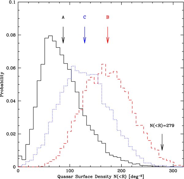
Figure 12. Measurement probability of the R < 22, z > 1.2 quasar surface density for various simulated sampling schemes meant to mimic our observations. Probabilities are computed based on simulated observations (N = 10,000) of the COMBO-17 CDFS field. The probability distribution expected from a random placement of 6 ≈80 arcmin2 fields is shown as case A (solid). The distributions resulting from a biased sampling in which the six fields are centered on known R < 22, z > 1.2 quasars are also shown. Case B (dotted) and C (dashed) histograms are the distributions with and without a central quasar correction. The mean values of each distribution are shown with arrows along with our measured surface density of N(R < 22; z > 1.2) = 279 (per square degree). Even the extreme biased sampling case is not able to reproduce our measured FLS quasar surface density.
Download figure:
Standard image High-resolution imageTo test the impact of biased sampling, rather than drawing random positions, we center each of six sub-fields on a known quasar within the desired flux and redshift range. This distribution (Case B) is meant to model the hypothetical situation that we previously ruled out, in which our primary targets are high-redshift quasars. Additionally, we compute the distribution from the same sub-fields, but with the targeted quasar excluded from the integrated counts (Case C). This last method provides an estimate for the situation in which our primary targets are not high-z quasars, but still trace regions of quasar overdensity. These biased simulations produce as much as a 2 × overdensity relative to the field average; however, neither adequately reproduces the measured FLS quasar surface density. The more realistic of these scenarios (Case C), in which the targeted ULIRGs might be tracing high-redshift overdensities, returns a <0.07% probability of measuring a surface density of 279 per square degree or higher. These results suggest that we are measuring a true overdensity of luminous (R > 22), high-redshift (z > 1.2) quasars in the FLS field. Whether this is simply due to cosmic variance or a selection bias in the COMBO-17 selection requires further investigation.
5.2. 2SLAQ/2QZ/6QZ
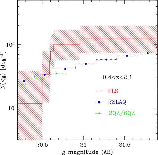
We also compare our sample to those of 2QZ/6QZ (Croom et al. 2004) and 2SLAQ (Richards et al. 2005), which offer complimentary quasar selections to that of COMBO-17. In contrast to the 17-band template fitting approach of COMBO-17, these employ UV–optical color selections with spectroscopic follow-up. One consequence of this difference is that they have different redshift sensitivities. Whereas COMBO-17 claims to have a uniform sensitivity above z > 1.2, the ultraviolet excess (UVX) approach is known to suffer from serious incompleteness at z ≈ 2.7, where quasars and main sequence stars are seen to be degenerate in UVX color space. Our 24 μm plus optical spectroscopy suffers no such catastrophic redshift bias, so we should have a fairly uniform census of AGN over all redshifts.
In Figure 13, the comparison between our g < 21.75 sample (2SLAQ limit) and the aforementioned UVX surveys is shown. The g-band photometry in this case is based on SExtractor AUTO magnitudes obtained with the Palomar large-field mosaic camera. We restrict our sample to redshifts 0.4 < z < 2.1 to match the sensitivities of the UVX surveys, but again apply no additional morphology, luminosity, or color selection. We do, however, apply an additional correction to our surface densities to account for a ≈20% g-band coverage incompleteness. This recovers an initial sample of eight AGNs with 0.4 < z < 2.1 and 18.0 < g < 21.75. One of these sources is an extended, low-redshift (z = 0.46), low-luminosity Seyfert that we exclude from the following comparison. The remaining seven sources all exhibit quasar-like luminosities and near stellar profiles (SExtractor stellarity >0.8).
Figure 13. Cumulative AGN surface density as a function of g-band magnitude. The AGN distribution is limited to sources with 0.4 < z < 2.1 (solid). This redshift constraint allows for the direct comparison to 2SLAQ and 2QZ/6QZ surface densities (Richards et al. 2005; Croom et al. 2004; dotted and dashed, respectively). In this redshift range, our derived surface densities are 2 × higher than either of these UVX-selected surveys. The 1σ confidence interval, shown as a hashed region, is based on small number Poisson statistics (Gehrels 1986).
Download figure:
Standard image High-resolution image
As in the COMBO-17 comparison, we suffer from poor number statistics at the bright fluxes. The integrated counts down to the SLAQ limit (g < 21.75) corresponds to a 2 × overdensity; however, due to the low counts, this carries only a 1.5σ significance. Examination of the UV–optical colors of these sources reveals that 6/7 sources have u–g versus g–I colors that are consistent with the 2SLAQ UVX color selection and one is significantly deviant, this is even without applying their full selection criteria, which includes a g–r and a morphology cut. Removal of this source brings the overdensity down to 1.7× at only a 1.2σ significance.
Based on this small sample, we infer that the initial overdensity is partially a real selection effect of the UVX survey. The magnitude of this bias is consistent with the 20% bias found by Brown et al. (2006) at brighter 24 μm fluxes (f24 > 1 mJy). After removal of this population, the resulting surface density is consistent with that of 2SLAQ.
6. SUMMARY
We use deep Keck optical spectroscopy to investigate the AGN sub-population of an N ≈ 300 24 μm selected galaxy sample (f24 > 200 μJy) in the Spitzer FLS. AGNs are classified based on the following emission-line diagnostics: (1) [N ii]/Hα versus [O iii]/Hβ, (2) [O iii]/Hβ, (3) [Ne v] strength, (4) and permitted emission-line line widths. Based solely on these classifications, AGN-dominated systems are identified over the redshift range 0 < z < 3.5. We use this sample to address the following questions. How does our spectroscopically selected, 24 μm AGN sample compare with that of an IRAC color-selected sample? What contribution do AGNs make to the overall 24 μm counts and flux density? How does our high-redshift AGN sub-population compare with those of recent wide-field optical/UV surveys?
Comparison of our sample with the four-color IRAC color selections of L04 and S05 confirms that at bright MIR flux levels, IRAC colors are an economical method for identifying AGN-dominated systems over a broad redshift range. Based on our spectroscopic identifications, we derive completeness and reliability estimates for the overall AGN sample of ≈70%/50% for the L04 colors and ≈50%/60% for the S05 colors. These fractions climb considerably when our sample is restricted to the MIR bright end of our sample. Given our survey's limited sensitivity to heavily obscured systems, the quoted reliabilities are lower limits for this flux range. The estimates for the overall sample do not adequately reflect the usefulness of the IRAC color selection for certain subsamples of the AGN population. In particular, the broad-line AGN population exhibits a very tight correlation in IRAC color–color space. Our completeness estimates for this sub-population are 90% and 70%, respectively, for L04 and S05.
Down to the flux limits of our Spitzer MIPS sample (f24 > 200 μJy), we find that 15%–20% of our targeted sources exhibit strong AGN signatures in their optical spectra. This population accounts for as much as 25%–30% of the integrated 24 μm flux from the population as a whole. This fraction is nearly 2 × higher than the 14.6% found by Fadda et al. (2002) over a comparable flux range using X-ray observations to identify the AGN population.
Isolating the optically bright end of our sample, we find that our quasar surface density is 3 × higher (5σ significance) than that of COMBO-17 over comparable optical flux (R <22) and redshift limits (z > 1.2). By contrast, over the lower redshift range (0.4 < z < 2.1), our quasar surface density is only marginally overdense relative to that of 2SLAQ (≈2 ×; 1.5σ significance), over a comparable optical flux range (g(AB) < 21.75). Part of this overdensity is attributed to optically reddened quasars that do not satisfy the 2SLAQ color selection. Of the quasars that overlap the optical and redshift limits, 6/7 have u, g, and i colors consistent with the 2SLAQ UVX color selection. Only one is significantly deviant, consistent with the 20% fraction found by Brown et al. (2006).
We thank the anonymous referee for the detailed and insightful comments that contributed greatly to the paper. This work is based (in part) on observations made with the Spitzer Space Telescope, which is operated by the Jet Propulsion Laboratory, California Institute of Technology under a contract with NASA. Some of the data presented herein were obtained at the W.M. Keck Observatory, which is operated as a scientific partnership among the California Institute of Technology, the University of California and the National Aeronautics and Space Administration. The Observatory was made possible by the generous financial support of the W.M. Keck Foundation. Support for this work was provided by NASA through JPL/Caltech contract 1287611. M.I. acknowledges the support from the Creative Research Initiative program, No. 2010-0000712 of the Korea Science and Engineering Foundation (KOSEF) funded by the Korea government (MEST). The analysis pipeline used to reduce the DEIMOS data was developed by the DEEP2 group at UC Berkeley with support from NSF grant AST-0071048. Finally, we wish to recognize and acknowledge the significant cultural role and reverence that the summit of Mauna Kea has within the indigenous Hawaiian community. We are grateful for the opportunity to conduct observations from this mountain.
Footnotes
- 5
For details of the FLS observation plan and the data release, see http://ssc.spitzer.caltech.edu/fls.
- 6