


ABSTRACT
We investigate the geometrical properties of energy release of synthetic coronal loops constructed using a recently published self-organized critical avalanche model of solar flares. The model is based on an idealized representation of a coronal loop as a bundle of closely packed magnetic flux strands wrapping around one another in response to photospheric fluid motions, much as in Parker's nanoflare model. Simulations are performed with a two-dimensional cellular automaton that satisfies the constraint ∇ · B = 0 by design. We transform the avalanching nodes produced by simulations into synthetic flare images by converting the two-dimensional lattice into a bent cylindrical loop that is projected onto the plane of the sky. We study the statistical properties of avalanches peak snapshots and time-integrated avalanches occurring in these synthetic coronal loops. We find that the frequency distribution of avalanche peak areas A assumes a power-law form  with an index αA ≃ 2.37, in excellent agreement with observationally inferred values and reducing error bars from previous works. We also measure the area fractal dimension D of avalanches produced by our simulations using the box counting method, which yields 1.17 ⩽ D ⩽ 1.24, a result falling nicely within the range of observational determinations.
Export citation and abstract BibTeX RIS
1. INTRODUCTION
In the last three decades a large amount of observational evidence had supported the idea that solar flares are generated by the storage and sudden, dynamical release of magnetic energy occurring in the solar atmosphere and lower corona. The very short observed timescales for flare onset point to magnetic reconnection as the most likely viable physical mechanism to convert magnetic energy to heat, although detailed quantitative models are still in the making.
Because the Sun's atmosphere is characterized by a high electrical conductivity, the stressing of magnetic field by fluid motions can press together magnetic flux surfaces of different magnetic orientations, and lead to the formation of electrical current sheets (e.g., Parker 1983). As the currents build up, magnetic reconnection sets in and causes a local topological reconfiguration and dissipation of the magnetic field within the current sheets. The many such currents sheets continuously undergoing reconnection everywhere in the corona power what amounts to a large number of very small flares. Parker (1988) estimated the energy release of one such elementary reconnection event at ∼1024 erg (and thus dubbed them "nanoflares"). In Parker's picture, stochastic photospheric fluid motions of convective origin shuffle the footpoints of magnetic coronal loops. With the frozen-in condition applicable within the loop to all but the very smallest spatial scales, in the low plasma-β characteristic of the corona the subsequent dynamical relaxation within the loop results in a complex tangled magnetic field essentially force-free everywhere except in numerous tangential discontinuities where strong current sheets build up and reconnection can set in.
On the observational front, numerous attempts have been made to verify of falsify Parker's nanoflare conjecture, and more specifically to extent flare observations, and determine distributions functions of their properties, all the way down to the nanoflare regime. One of the most remarkable observational facts derived from observed flare statistics is that the frequency distribution of the energy release takes the form of a tight power law spanning at least eight orders of magnitude in flare energy (see e.g., Dennis 1985; Aschwanden et al. 2000), indicative of self-similarity in the flaring process.
Motivated in part by this idea, Lu and Hamilton (Lu & Hamilton 1991) developed the first avalanching sandpile model of flaring active regions, which later gave rise to numerous variations on the same theme (Lu & Hamilton 1991; Lu et al. 1993; Georgoulis & Vlahos 1996; Georgoulis & Vlahos 1998; Charbonneau et al. 2001). All these models share common features, notably the fact that they are cellular-automaton (CA)-like, i.e., their spatiotemporal evolution is governed by discrete, simple local stability and redistribution rules. They all produce power-law distribution of avalanche energy, in many cases with logarithmic slopes comparing favorably to observations (see Charbonneau et al. 2001 for a review). However, all these models suffer from the same fundamental drawback, namely the difficulty in linking back in an unambiguous and quantitative manner their internal rules to the physical laws governing the evolution of coronal magnetic fields, namely magnetohydrodynamics.
In a recent paper Morales & Charbonneau (2008a) we presented a novel avalanche model of solar flares, using magnetic field lines as a basic dynamical element. While still CA-like in its use of local, discrete stability and redistribution rules, this model (1) can be unambiguously mapped onto a coronal loop, (2) allows the quantitative calculation of energy release in physical units, and (3) ensures by its very design that ∇ · B = 0. Our simulations showed that this driven dissipative CA evolves to a self-organized critical (SOC) state with avalanche of reconnection events collectively spanning a wide range of sizes and with frequency distribution of size parameters comparing to observations at least as well as earlier sandpile models.
Comparisons between geometrical properties of avalanches and flare observations at high spatial and temporal resolution are not abundant in the literature (McIntosh et al. 2002; McIntosh et al. 2001; Morales & Charbonneau 2008b; Aschwanden & Aschwanden 2008b; Uritsky et al. 2007). Nevertheless, all of them agree in suggesting that geometrical assumptions made in reconstructing the flaring volume from areas observed in the plane of the sky play a critical role when calculating the energy released by individual flares. Consequently, in this paper we investigate the geometrical properties of avalanches in our new SOC model for solar flares. To do this we reconstruct the cylindrical geometry of the coronal loop and study the geometrical properties and associated statistical distributions of projected avalanche areas.
In the following section we briefly review the design and operation of our recent SOC model for solar flares, and define the various geometrical measures to be used in what follows. In Section 3 we describe the sequence of transformation steps required to map our two-dimensional simulations results onto three-dimensional loop-like structures, which then allows us to synthesize pseudo-flare observations. Sections 4 and 5 are devoted to study the geometrical properties of projected avalanches. In Section 4 we calculate frequency distributions of flaring areas and in Section 5 we compute the fractal dimension of our synthetic solar flares by means of a box counting method. We summarize our results and conclude in Section 6.
2. THE STRAND-BASED MODEL FOR SOLAR FLARES
In this section we summarize the conceptually novel SOC model for solar flares we have recently developed. For full details concerning the model, implementation and numerical simulations, see Morales & Charbonneau (2008a). The model is basically an anisotropic CA that uses magnetic field lines as the main dynamical element. We define a two-dimensional regular Cartesian lattice of size N × N as an idealized representation of the outer surface of a straightened coronal loop. On this lattice we define a network of vertically interconnected nodes with periodic boundary conditions in the horizontal direction. Each vertical line so defined represents a magnetic flux strand (or tube), i.e., a bundle of magnetic fieldlines behaving as a coherent entity. Driving is introduced in the form of sequential, horizontal displacements (with nonzero mean) at randomly selected single nodes, mimicking the effects of random photospheric footpoint displacements propagating within the loop. Over time each node ends up executing a form of biased random walk that inexorably leads to an increase in the length of the flux strands, which, via mass and flux conservation within each strand, leads to an increase in the magnetic energy content of the strands. Consequently, the total magnetic energy collectively stored within all strands defines the lattice energy.
After many steps of this driving process, there will also inevitably come a point where two or more flux strands "cross" at certain lattice site, jointly subtending an angle hereafter denoted Θ. We use the value of this angle as a stability criterion, as suggested by theoretical considerations (Parker 1988), which have recently found support in numerical simulations (Dahlburg et al. 2005); whenever Θ exceeds some preset threshold Θc, we cut-and-splice the two flux strands and displace one of the two nodes away from the unstable site, in such a way that the magnetic energy of the system decreases. This, in turn, can lead to the formation of new unstable crossing angles at neighboring lattice sites, which are then themselves spliced and displaced, and so on in classical avalanching style. As in other "stop-and-go" classical SOC sandpile models, driving is suspended during the avalanche, mimicking in this way, the existing separation of timescales between photospheric driving (of the order of minutes to hours) and flare onset (seconds). In Figure 1 we illustrate the operation of the CA for a very small lattice.

Figure 1. Detail of a small lattice showing the basic lattice structure and driving mechanism. The "photosphere" corresponds to the top and bottom horizontal rows of nodes. Strands are numbered from left to right and nodes along a given strand, from bottom to top. In the left plot, node (2, 6) of strand 2 has been displaced two units to the right and for strand 6 the node (6, 6) has been displaced two units to the left. Both strands meet at the highlighted node (4, 6) forming an angle Θ = 4.1 rad>Θc. The actual first neighbors of node (4, 6) are shown as squares. In the right plot the redistribution rule has been applied and strands 2 and 6 have `reconnected' and a new unstable angle is formed at node (3, 6). Periodic boundary conditions are enforced in the horizontal direction, so that strands 1 and 8 always experience the same displacement (here one unit to the right).
Download figure:
Standard image High-resolution imageIn Morales & Charbonneau (2008a) we showed that this model produces spatially and temporally intermittent, avalanche-like release of magnetic energy, with frequency distributions of avalanche size parameters in the form of power laws with logarithmic slopes comparing well to observationally inferred values. We also calculated the so-called spreading exponents η and δ and verified that they satisfy the mutual numerical relationship expected from SOC, thus indicating that this CA does behave as a SOC system (Morales & Charbonneau 2008b).
In the present paper we take advantage of the unambiguous mapping onto loop-like structures that is possible within our model to synthesize artificial images of flaring loops, arbitrarily oriented with respect to the heliocentric radius vector and projected against the plane of the sky. This yields a geometrical setup that is entirely analogous to the way in which spatiotemporally resolved flare observations are analyzed.
3. FROM A TWO-DIMENSIONAL LATTICE TO A SYNTHETIC CORONAL LOOP
Our simulation is defined over an horizontally periodic two-dimensional Cartesian plane representing the outer surface of a "straightened" coronal loop, with the vertical direction parallel to the loop axis. To generate a three-dimensional synthetic coronal loop with appropriate shape, aspect ratio and orientation, we need to apply a sequence of transformations to our two-dimensional lattice: (1) wrapping into a cylinder; (2) stretching along the cylinder's axis; (3) bending in half into a loop-like structure; (4) rotate in a plane having an arbitrary orientation with respect to the line-of-sight; (5) project into the plane of the sky as a pixel image.
We first define a reference right-handed coordinate system where the coordinate z is in the vertical direction and the x, y coordinates define the photospheric plane. Assuming that the two-dimensional lattice is located at the plane y = 0, as shown in Figure 2(a), the nodes (i, j) can be written in terms of the three-dimensional coordinate system as (0, i, j). We then calculate the new loop coordinates of the wrap/stretched/bended lattice (xL, yL, zL) by performing the mathematical transformation detailed in the Appendix.
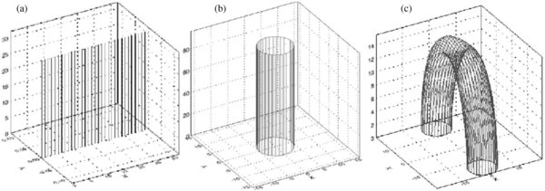
Figure 2. Pictorial representation showing how a two-dimensional lattice is converted in a cylinder and then bended in a loop. (a) Original two-dimensional lattice of linear size N = 32. (b) The formed cylinder that has tripled in length (Δ = 3). (c) A possible view of the synthetic coronal loop, after bending with R = (N − 1)/π.
Download figure:
Standard image High-resolution imageWhen analyzing microflares Aschwanden et al. (2000) suggested that observations are the projection of the flaring volume of a cylindrical loop onto the plane of the sky. With our model we can project the three-dimensional coordinates of the flaring nodes within the synthetic loop into any chosen plane by simply applying a projection matrix P to the vector (xL, yL, zL). The projection matrix can be easily expressed in terms of the components of the vector  normal to the projection plane: aX + bY + cZ = 0.2 For such a plane the corresponding projection matrix is
The projected coordinates of any given three-dimensional point belonging to the synthetic loop will be (xp, yp, zp) = P(xL, yL, zL).
We then produce a synthetic equivalent of an observed flare by covering the projected loop by a two-dimensional Cartesian grid of contiguous square pixels, and simply sum the number of avalanching nodes falling within each individual pixel, which then becomes a proxy for emitted flux. The upper panel of Figure 3 shows an example of a moderately large avalanche on a 32 × 32 lattice. Each solid dot corresponds to a node having avalanched at least once in the course of this event. The lower panel of Figure 3 (left) shows a 16 × 16 grid pixellization of the event illustrated above, with the dotted square showing the area in the plane of the page covered by this pixellization. The gray scale encodes the number of avalanching nodes falling within each pixel. The resulting synthetic image is clearly dependent on the assumed orientation of the loop, as can be seen by comparing the two projections depicted in the lower part of Figure 3, which shows the pixellization corresponding to a different projection of the same avalanche.
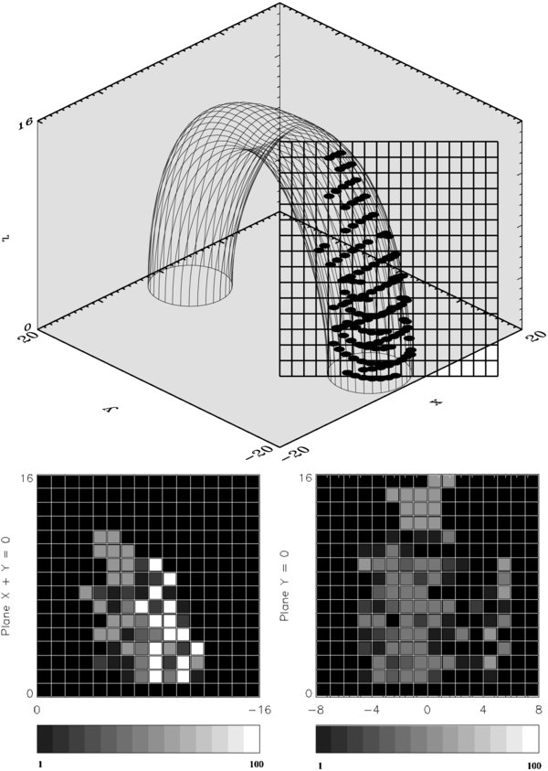
Figure 3. Synthetic flare structure for a 32 × 32 lattice converted in a synthetic coronal-loop (up). In this case Δ = 1 and R = (N − 1)/π. Each dot indicates a lattice node having became unstable at least once in the course of this avalanche The plane of projection X + Y = 0 is superimposed. The two bottom images show two (coarse) pixellizations of this synthetic flaring loop, for the planes defined by X + Y = 0 (left) and Y = 0 (right). The gray scale encodes the number of unstable nodes along the line of sight associated with each individual pixel (see the text).
Download figure:
Standard image High-resolution imageEvidently, the synthetic flare image associated with a given avalanche will also depend at least to some degree on the chosen values for the various numerical parameters involved in the wrapped/stretch/bend/project/pixellize sequence of steps described above. As an example of the range of possible "flare images" that can be produced from the same avalanche, consider the six synthetic images displayed in Figure 4, all produced from the same large avalanche on a lattice of 128 × 128 with a threshold angle Θc = 2. This avalanche lasted 1094 iterations, and involved a grand total of 1142 nodal energy release events, with 113 unstable nodes at the time of peak energy release. The synthetic images displayed in the left column are produced by using the distribution of time-integrated avalanching nodes, i.e., all the nodes that were unstable at least once during the life time of the avalanche. The middle column uses the distribution of avalanching nodes at the time of peak energy release. All images are projections in the plane X + Y = 0 and use two different values of the radius of curvature. For the first four panels R = (N − 1)/π and for the two bottom panels R = 100(N − 1)/π the loop length being respectively N − 1 and 100(N − 1). The first two rows use a stretching factor of Δ = 1 but two different levels of pixellization (12 × 12 versus 24 × 24). The bottom row retains the 12 × 12 pixellization, but now uses a stretching factor Δ = 100, i.e., 100 times that used to produce the images in the top and middle rows. As a visual comparison point, the three images displayed in the right column are TRACE observations of very small flares, taken from Aschwanden et al. (2000). For the synthetic flare displayed in the bottom row, the combination of high level of stretching (Δ = 100) and coarseness of the pixellization (12 × 12) washes out all internal structure, leaving only the same projected shape of the bent loop visible on either the time-integrated or peak energy release images. The examples displayed in Figure 4 illustrate that our synthetic flare images show a type of general structure that is at least qualitatively similar to observational results. This motivates the more quantitative comparisons to which we now turn.

Figure 4. "Observational" views of the projections of the time-integrated avalanches (left panels) and at the avalanche peak (central panels) and TRACE observations performed by Aschwanden et al. (2000; right panels). The two upper panels show the X + Y = 0 projection for a 128 × 128 lattice and Θc = 2 rad. The only difference between the first and second row panels is the pixel size. The third row panel shows the same set of nodes that took part in the avalanche but for loop longer loop (R = 100(N − 1)/π and Δ = 100). The pixel size is the same that in row number 2. The three images in the right column were kindly provided by M. Aschwanden.
Download figure:
Standard image High-resolution image4. STATISTICAL PROPERTIES OF PROJECTED AVALANCHES
Isotropic sandpile-like avalanche models of solar flares as well as our strand-based avalanche model both succeed in producing power laws for the probability distribution of avalanche areas. In the classical isotropic models the associated power-law index turned out much smaller than observationally inferred values (see e.g., McIntosh et al. 2002), while our recent SOC model yields numerical values in better agreement with observational inferences. However, this better agreement may be fortuitous to some extent, since the flaring areas were calculated directly in the two-dimensional Cartesian lattice, which is not a one-to-one representation of the observational plane. Following the sequence of steps described in the preceding section we are in a position to synthesize observations in a plane equivalent to the plane of the sky, and revisit this question in a more meaningful manner.
Starting from long simulation runs on lattices of various sizes, we calculate the avalanche areas for two different cases. The first case corresponds to the area covered by all the nodes that were unstable at least once in the course of the avalanche: the so-called time-integrated area and the second corresponds to the area covered by all the nodes unstable at the moment of the avalanche peak. For both cases we calculated the projections on the four planes defined by the equations: X + Y + Z = 0, X − Y = 0, X + Y = 0, and X − Z = 0. Not surprisingly, the frequency distributions of projected avalanche areas are found to take the form of well defined power laws, spanning over 2 orders of magnitude in area. A representative example is presented in Figure 5 for the case of a 128 × 128 lattice with Θc = 2.25. Distributions are calculated for both time-integrated area and area at time of peak energy release (cf. Figure 5). The top three lines of Table 1 compile the corresponding power-law indices for time-integrated areas (α*A) and peak area (αA) for three different lattice sizes. The error presented corresponds to the maximum one sigma uncertainty obtained by a least-squares linear fitting. Having established previously that the statistical properties of avalanches do not depend on the threshold angle (Θc; see Morales & Charbonneau 2008a, 2008b), all results presented in Table 1 used as threshold angle Θc = 2 rad. Whether working with time-integrated avalanches or peak snapshots, within error bars the inferred power-law indices are independent of lattice size, as one would expect from a SOC system.
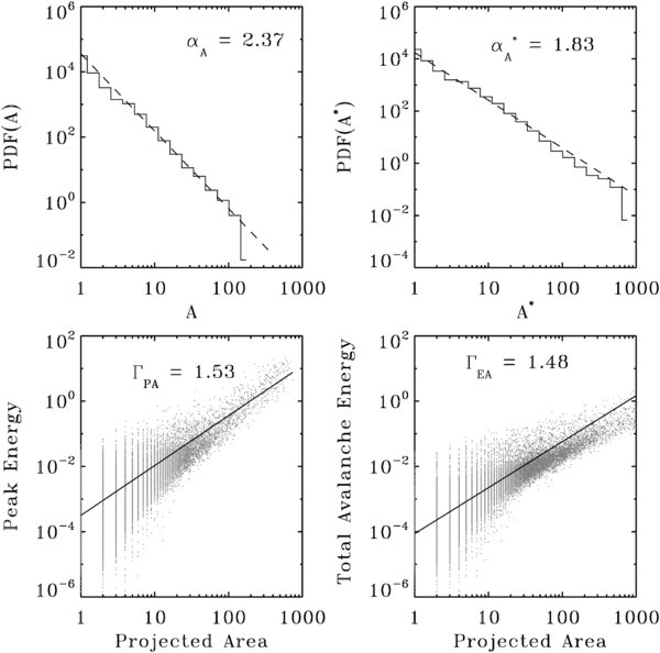
Figure 5. Illustrative case of the frequency distribution obtained for the projected area both for the time-integrated avalanches (top-right) and for the avalanche peak (top-left). In this case we worked with a 128 × 128 lattice a threshold angle Θc = 2.25 rad and Δ = 1. These correlation plots are constructed from ∼2.2 104 distinct avalanches. The two lower plots show the correlation between avalanches area and total released energy. The plot on the left shows the correlation between energy release and area at the time of peak energy release, while the plot on the right shows a similar plot for the time-integrated area and energy release over the duration of each avalanche.
Download figure:
Standard image High-resolution imageTable 1. Power-law Indices for Correlation Plots for Series of Lattice Simulations for Different Lattice Sizes and Compilation of Previous Results
| N | αA | α*A | ΓEA | ΓPA |
|---|---|---|---|---|
| 32 | 2.31 ± 0.09 | 1.73 ± 0.08 | 1.57 ± 0.15 | 1.37 ± 0.15 |
| 64 | 2.32 ± 0.09 | 1.73 ± 0.08 | 1.65 ± 0.10 | 1.56 ± 0.1 |
| 128 | 2.37 ± 0.09 | 1.83 ± 0.08 | 1.48 ± 0.10 | 1.53 ± 0.08 |
| LH-2D (64) | 1.05 ± 0.07 | 0.52 ± 0.03 | 1.07 ± 0.05 | 1.04 ± 0.04 |
| LH-2D (128) | 1.02 ± 0.06 | 0.55 ± 0.02 | 1.06 ± 0.04 | 1.04 ± 0.04 |
| LH-3D (64) | 1.12 ± 0.05 | 0.63 ± 0.03 | 1.59 ± 0.04 | 1.07 ± 0.03 |
| TRACE 19(A) | 2.16 ± 0.18 | |||
| TRACE 195(B) | 2.25 ± 0.04 | |||
| TRACE 171(A) | 2.45 ± 0.09 | |||
| TRACE 171(B) | 2.34 ± 0.09 |
Download table as: ASCIITypeset image
The three lines of Table 1 identified as LH-2D and LH-3D list the corresponding power-law indices for a selection of two-dimensional and three-dimensional simulations using the Lu & Hamilton isotropic sandpile model, as taken from McIntosh et al. (2002). In the three-dimensional case the areas correspond to projections on the three Cartesian planes of the lattice cube, while for the two-dimensional simulations is just the area of the avalanching region (as in Figure 4 herein). In the last four lines of Table 1 we reproduce the results presented in Table 3 of Aschwanden & Parnell (2002). In that table they used TRACE data obtained in two wavelengths (195 Å and 171 Å) on two dates. The campaign (A) took place on February 24th of 2000 and produced a database of 816 flare events (436 observed at 171 Å and 380 observed at 195 Å) with flare energies going from microflares all the way to nanoflares as shown in Figure 10 in Aschwanden & Parnell (2002). Campaign (B), on the other hand, took place on 1999 February 17. In this case, they registered 281 flare events with energies spanning a range going from 1024 erg to 1032 erg (see Aschwanden & Aschwanden 2008a) and measured the equivalent of the flare peak avalanching areas.
We also studied the correlation between the projected areas and the energy liberated by each avalanche. We found tight power laws extending over at least three to four orders of magnitude as illustrated in Figure 5. Aschwanden & Aschwanden (2008a) calculated the correlations measures between area and total emission measure and between area and thermal energy (Figure 7). They obtain correlation exponents of 1.539 and 1.634 respectively. These values are in agreement with those presented in the fourth column of Table 2.
Table 2. Area Fractal Dimension D for Different Lattice Sizes and Stretching Factors
| N | D | Δ |
|---|---|---|
| 32 | 1.28 ± 0.07 | 1 |
| 64 | 1.24 ± 0.08 | 1 |
| 128 | 1.34 ± 0.08 | 1 |
| 32 | 1.20 ± 0.07 | 10 |
| 64 | 1.19 ± 0.06 | 10 |
| 128 | 1.17 ± 0.07 | 10 |
| 32 | 1.12 ± 0.05 | 30 |
| 64 | 1.11 ± 0.06 | 30 |
| 128 | 1.12 ± 0.05 | 30 |
| 32 | 1.03 ± 0.04 | 100 |
| 64 | 1.06 ± 0.04 | 100 |
| 128 | 1.08 ± 0.05 | 100 |
| LH-2D(64) | 2.02 ± 0.05 | ≡1 |
| LH-2D(128) | 2.01 ± 0.06 | ≡1 |
| EIT/SOHO (Uritsky et al. 2001) | 1.5 ± 0.1 | ≡1 |
| EUV 171 Å (Aschwanden & Aschwanden 2008a) | 1.34 ± 0.24 | ≡1 |
Download table as: ASCIITypeset image
Having obtain a first evidence of the utility of the synthetic avalanching loop as a tool to model solar flares we turn now to a pure geometrical property of avalanches: the fractal dimension.
5. FRACTAL DIMENSION OF PROJECTED AVALANCHES
Solar flares have fractal and filamentary structure. Thermal energy or electron density can be determined more accurately when the volume fractal dimension or the filling factor is know (Aschwanden & Aschwanden 2008a). In the last 20 years several observational determinations of the flaring area's fractal dimension D have been carried out using different kinds of data such as photospheric magnetograms, EUV and soft X-ray images of nanoflares, and EUV images of the quiet Sun. The inferred values of D cover an extremely broad range, down from 1, corresponding to linear objects, to 1.93, i.e., almost a pure two-dimensional object (see Table 1 in Aschwanden & Aschwanden 2008a and references therein). Essentially all of these determinations use one of two approaches: calculating the area/volume or radius/area relationship, or the box-counting method.
For numerical avalanche models of flares, on the other hand, there exist comparatively few determinations of the fractal dimension. Only McIntosh et al. (2001) and McIntosh et al. (2002) have performed estimations of the fractal dimension using the ratio of area to linear dimensions. They obtained fractal index values in the range 1.55 ⩽ D ⩽ 1.79 for peak area, and D ≃ 2 in the case of time-integrated avalanche areas.
Calculating the fractal dimension of structures is analogous to measuring the length of a curve, the area of a surface, or the volume of a three-dimensional object. To do this one calculates the number of segments, or squares or cubes (depending on the structure's Euclidean dimension) of size δ needed to cover the whole structure. For the case of a segment of length L:

where N(δ) is the number of segments needed to cover the line of length L. If L = 1 then N(δ) = 1/δ. In the same way for a unit square N(δ) = 1/δ2 and for a unit cube N(δ) = 1/δ3.
To characterize more complicated geometric structures one may calculate its Hausdorff–Besicovitch fractal dimension (for a complete description, see Mandelbrot 1977, Feder 1988, and Schuster 1989). A straightforward way of estimating the Hausdorff–Besicovitch fractal dimension is the box counting method. Essentially this method consist in calculating the number of squares of size δ needed to cover the structure of interested assuming that the frame containing such a structure is of unit size. Under this circumstances,
from which
In order to estimate the value of D for the avalanches produced by our simulations we applied the following procedure: we start with a bitmap of the pixellized images associated with some chosen projection plane, as produced following the procedure described previously in Section 3. Two representative examples are shown in the leftmost column of Figure 6, for a reference pixel size δ = 1/32. White (black) pixels are those in which no (at least one) active lattice node is mapped for the chosen mapping and projection parameters. The middle and rightmost column show the result of the same procedure applied with pixels of successively doubled size (δ = 2/32 and δ = 4/32). It is then just a matter of counting the number N(δ) of black pixels associated with each pixellization, and using Equation (4) to compute D.
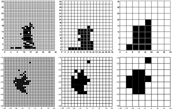
Figure 6. Box counting method displayed for two different lattices. In the upper figure we present the XZ projection of an avalanche produced in a 32 × 32 lattice. The avalanche involves 771 nodes and lasted 217 iterations. The lower figure presents the XY projection of an avalanche produced in a 64 × 64 lattice. The avalanche involves 2541 nodes and lasted 190 iterations.
Download figure:
Standard image High-resolution imageOne should rightfully expect that the computed values of D will depend on choices made for the numerical parameters used in converting our two-dimensional Cartesian lattice to a bent loop-like structure, and in particular on the stretching factor Δ. Table 2 lists the computed values of D for sets of simulations carried out on three different lattice sizes, for values of Δ varying from unity (thick short loop) to 100 (thin long loop) that corresponds to radius varying between ∼40 and 4000. For a given lattice size, the "database" of avalanches is always the same, and so are the projection planes used to construct the synthetic flare images. The error represents the maximum standard deviation from the mean value.
To exemplify the typical results obtained by calculating D for the different values of pixel size δ we have produce Figure 7. There we display the mean value of D calculated by applying Equation (4) to more than 500 avalanches that lasted at least 50 iterations. We worked with five different pixel sizes for a lattice of size N = 128 and for with three different pixel sizes for lattices of size N = 32 and N = 64.
Figure 7. Mean value of the fractal dimension calculated for lattices of size N = 32 and N = 64 for three different values of δ = [1/32, 2/32, 4/32] (triangles and diamonds respectively) and calculated for a bigger lattice of size N = 128 using five values of δ = [1/32, 1/24, 2/32, 2/24, 4/32] (squares).
Download figure:
Standard image High-resolution imageFor a given value of Δ, the calculated fractal dimension is independent of lattice size within error bars, as expected from the self-similarity characterizing avalanching dynamics in the model. Even at Δ = 1 the inferred fractal dimension D is far from the Euclidean limit D = 2; this is not surprising since a large fraction of the simulated avalanches tend to exhibit an elongated structure, a direct consequence of the strongly anisotropic nodal connectivity on the lattice. This leads to fractal dimension that look more like nearly unidimensional structures, such as the Koch's curve: D = 1.2618 (see, e.g., Figure 2.8 in Feder 1988).
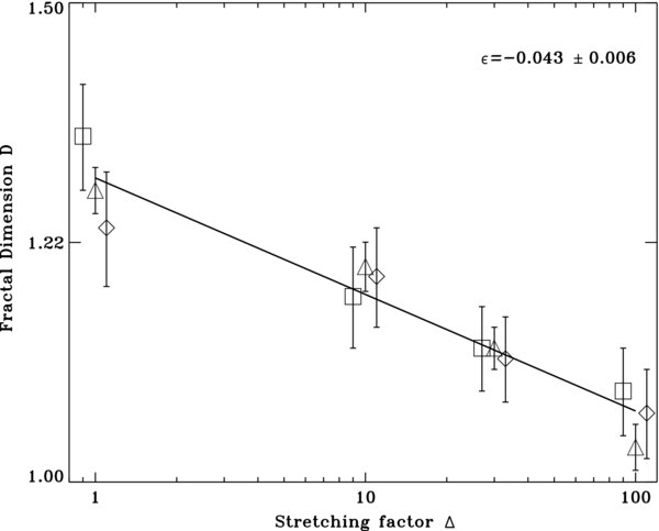
In Figure 8 we plot the fractal dimension (D) versus loop stretching Δ, for various lattice size, as coded by the various symbols. All these data can be well fit by a power-law relationship of the form

with a least-squares fit yielding a power-law slope  = −0.043 ± 0.007. The proportionality constant in this case, D0, is the value of the fractal index when the synthetic loop experiences no stretching (Δ = 1). That the fractal dimension should then toward unity as the loop is stretched to very large aspect ratio is of course not surprising. What is noteworthy is that even for rather large stretching factors (many tens), the flaring area retain a markedly nonlinear fractal dimension (D ≃ 1.2 at Δ = 10).
Figure 8. Best fit to Equation (5) obtained by performing linear regression analysis on the three different set of simulation results compiled in Table 2: triangles for a 32 × 32 lattice, diamonds for 64 × 64 and squares for the 128 × 128.
Download figure:
Standard image High-resolution image
Recent high time cadence observations presented by Aschwanden & Aschwanden (2008a) showed that the fractal dimension of flaring areas evolves with time with values ranging between [1, 1.64] for the initial fractal dimension, up to [1.78, 1.97] for the fractal dimension corresponding to the moment of maximum area. Since our model does not simulate the thermalization phase occurring in flares and we can only reproduce the initial energy release at flaring onset event, we believe that our results should be compared to the fractal dimension values obtained at the onset of the flare. Inspection of Table 2 of Aschwanden & Aschwanden (2008a) shows that 1 ⩽ D ⩽ 1.31 for 6 out of 10 of the initial fractal dimension values for the M-Class flares (see also their Figure 10), with the mean value of the whole data set 〈D〉 = 1.34 ± 0.24. This would suggest that our shorter loops offer a better geometrical representation of observed flares.
In Table 2 we also presented the results obtained by Uritsky et al. (2007). In that case they calculated the fractal dimension for an EUV-bright region at the peak of a brightening event. They identify an avalanching region as the region where EUV flux exceeded a certain threshold. For more than 7000 EIT images collected by SOHO in the 195 Å wavelength, they obtain D = 1.5 ± 0.1 for both solar maximum and minimum. This value is closer to that inferred by Aschwanden & Aschwanden (2008a) for the epoch of peak energy release than for the epoch of flare onset which, we believe, is more appropriate for comparison with our synthetic images.
6. SUMMARY AND DISCUSSION
In this paper we have generated synthetic flare-like spatiotemporal energy release events using the novel SOC avalanche model described in Morales & Charbonneau (2008a). This model is based on a two-dimensional isotropic CA designed to offer an idealized representation of a coronal loop, and, geometrically and operationally, is very much along the line of the physical picture of nanoflares proposed by Parker (1983, 1988). By virtue of its design, this avalanche model can be mapped onto a geometrically realistic coronal loop without ambiguity with regards to the physical correspondence of model elements. A sequence of straightforward transformations can then turn an avalanche taking place on the two-dimensional lattice into an avalanche occurring within a three-dimensional curved loop-like structure with realistic aspect ratio. This can then be projected at arbitrary angles onto the plane of the sky and turned into a two-dimensional pixel intensity image akin to those produced by high resolution EUV and X-Ray imaging instruments.
We have focused here primarily on the geometrical properties of synthetic flares images produced by our SOC model. In particular, we have computed the frequency distribution of flaring areas, which was found to take the form of a well defined power law with a logarithmic slope αA = 2.35 comparing very well to the observationally inferred value (1.86 ⩽ αA ⩽ 2.45, see e.g., Aschwanden & Parnell 2002), unlike earlier SOC models of flares based on conventional, isotropic sandpile-like CAs. This is a robust result that was found to depend very little on the adopted lattice size and other model parameters, or on the assumed aspect ratio for the loops. As shown in Morales & Charbonneau (2008a), this model also yields frequency distribution of flaring energy, peak flux, and duration that also compare favorably to observations.
We also studied the fractal dimension of our synthetic flares images. We first established that these images do obey the self-similar scaling expected of fractal structures, and then obtained a fractal dimension (D) in the narrow range 1.1 ⩽ D ⩽ 1.34, with the lower bound corresponding to "long thin loops" with length-to-diameter aspect rations of up to 100:1, and the upper bound to "short fat loops" with aspect ratio of order unity. This range compares quite well to the mean fractal dimension D = 1.34 inferred observationally using data from Aschwanden & Aschwanden (2008a) for M-Class flares.
The good agreement between the observed geometrical properties of real solar flares and their synthetic counterpart produced by our model suggests that the latter, despite its (relative) simplicity, could serve as a bridge between spatiotemporally resolved observations of flare energy release and the microscale physical processes underlying the flaring phenomenon, most notably magnetic reconnection, that are below the resolution limit of current and forthcoming instruments. In our model, the unfolding of an avalanche is intimately tied to the discrete rules introduced to mimic magnetic reconnection and destabilization of neighboring nodes. In principle, different reconnection scenarios could translate into different choices for these discrete rules, and therefore into distinct avalanching dynamics. Observational constraints on the latter then become constraints on the small-scale microphysics underlying the discrete rules. Conversely, we think that the synthetic flares produced by our model could be helpful in testing numeric algorithms for the automatic detection and tracking of flare energy release. We may be able to use the localized nodal energy release produced by our model as input to one-dimensional thermalization models of coronal loop (Klimchuk 2008), in order to synthesize actual EUV emission measures that would be comparable in detail to spatiotemporally resolved flare observations.
The fact remains that CA models such as the one used here remain far removed from the plasma and magnetohydrodynamical processes collectively producing what we call flares. Yet, these models evidently catch some essential aspect of the process. Self-similarity in energy release statistics and a non-integer, fractal dimension for the flaring volumes all hint that solar flares represent yet another instances of physical phenomena increasingly becoming known under the name of natural complexity. The hallmark of such systems is a global dynamical behavior governed by local threshold-interactions between a large number of degrees of freedom. Without denying the fact that the physical heart of the flaring process, magnetic reconnection, would be better described by magnetohydrodynamics rather than largely ad hoc discrete interaction rules, natural complexity offers a higher level framework unifying processes taking place in very different physical systems (Uritsky & Klimas 2004). As a case in point, it should be noted that energy release in the earth's magnetotail is increasingly being viewed as yet another instance of natural complexity (see, for example, Uritsky et al. 2001 and Uritsky & Klimas 2004), and modeling frameworks similar to that used here are gaining more and more recognition as viable descriptors of magnetospheric substorms (see, for example, Chang 1992, Liu et al. 2006, and references therein).
Many developments of our model are still possible, notably the generalization to a truly three-dimensional cylindrical lattice, which would allow the introduction of driving rules that would incorporate a preferred direction of twist. At a more theoretical level, it would be interesting to investigate whether our line-based, anisotropic CA belongs to a universality class distinct from the curvature-triggered isotropic sandpile models that have dominated the modeling of flares as avalanches of elementary reconnection events. Improved synthesis of pseudo-flare statistics could also make use of some of the loop parameter scalings established observationally (see, e.g., Aschwanden et al. 2000).
This research is supported in part by the Natural Sciences and Engineering Research Council (Canada) and by the Fond Québécois pour la Recherche sur la Nature et les Technologies (Québec).
APPENDIX
In this appendix we present in full detail the mathematical steps followed to transform the lattice two-dimensional coordinates into loop-coordinates as illustrated in Figure 2.
In order to obtain the loop coordinates of the originally two-dimensional lattice nodes we begin by wrapping the two-dimensional lattice around a vertical axis and placing the resulting cylinder so that its symmetry axis coincides with the (x, y) = (0, 0) line, as shown in Figure 2(b). Since the length unit on the lattice is by definition the internodal distance, the total width of a N × N lattice is N − 1; assuming that this is the total perimeter of the cylinder, then its radius is simply
Since the total angle covered by the nodes in the cylinder is 2π we can estimate the angle separation ϕ between node i and the i = 0 node as
Thus the new cylindrical coordinates of a node (i, j) will be


In order to bring the model closer to the real aspect ratios characterizing coronal loops we can stretch the cylinder by multiplying the z coordinate by a constant Δ, so that we now have

with Δ>1 since the length of coronal loops is typically much larger than their cross-section. Figure 2(b) shows the end result of the wrap and stretch steps. We must now proceed with the (mathematically trickier) bending step. To do this we assume that the total height of the cylinder is the typical length of the synthetic loop and thus determines (RL), so that
The angle formed between each node and the XY plane will be
Thus, the new coordinates for each node belonging now to the (bent) loop axis lying in the X = 0 plane are


The result of this bending step is shown in Figure 2(c). The calculated loop coordinates can then be projected in any desired plane by following the procedure described in Section 3.
Footnotes
- 2
This is the case for a plane passing through the origin (0, 0, 0) of the Cartesian coordinate system. We can work under this assumption without any loss of generality.