


ABSTRACT
Results of 974 speckle observations of 546 binary stars are presented. Observations were obtained at the WIYN 3.5 m Telescope at Kitt Peak National Observatory during the time interval from 2007 January to 2008 June. In all cases, the relative separation and position angle of the components are measured, and the magnitude difference is determined in 809 cases. The precision of the results as judged from repeat observations and objects with very well-determined orbits is similar to previous papers in this series, namely ∼3 mas in separation and <1° in position angle in most cases. Similarly, the photometric precision remains consistent with previous WIYN speckle data, on average ∼0.1 mag per observation. Six systems of special interest are discussed.
Export citation and abstract BibTeX RIS
1. INTRODUCTION
The WIYN speckle program has now entered its second decade, having commenced observations in 1997 with two detectors for recording speckle images: a multi-anode microchannel array (MAMA) detector, provided by J. G. Timothy (Nightsen, Inc.), and a fast-readout CCD, provided by Z. Ninkov (Rochester Institute of Technology). The goals of the program were to obtain high-precision relative astrometry and photometry of subarcsecond visual double stars, particularly those discovered by Hipparcos, prioritized by distance. (First results were presented in Horch et al. 1999, Paper I in this series.) Such observations are vital for obtaining orbital elements of the systems that are gravitationally bound as well as making determinations of mass sums. The latter can be obtained by using the parallaxes appearing in the Hipparcos Catalogue in addition to the relevant orbital elements.
The combination of both a microchannel plate-based detector and a CCD gave us a unique opportunity to understand and disentangle the problems with the photometry typically obtained in speckle observations up to that time. This has been an important focus of the program, since reliable photometry would allow for the precise determination of the magnitudes and colors of the components of observed systems. With this information, substantial progress can be made on understanding the details of the mass–luminosity relation and stellar evolution calculations. The CCD camera, aided by the superb median seeing conditions at WIYN (∼0.8 arcsec), has been able to give reliable differential photometry in the case of many observations, as discussed in Horch et al. (2004) and Horch et al. (2008) (Papers IV and V of this series). Therefore, only the RIT CCD was used from 1998 through 2006. Photometric information obtained during this time frame has been recently used to make comparisons with stellar evolution calculations in Davidson et al. (2009).
In 2001, the efficiency of our observational program was increased with the advent of the RIT-Yale Tip-tilt Speckle Imager (RYTSI), described in Meyer et al. (2006). The RIT chip has a format of 2033 × 2048 pixels, much larger than is needed for speckle observations, and prior to 2001 much of this detector area was unused in speckle observations. By including a two-axis galvanometer scanning mirror system in the RYTSI optics package before the detector, it became possible to use the entire area of the chip as a physical memory cache of speckle frames. This is accomplished by executing a serpentine step-and-expose pattern with the galvanometer mirrors.
The work presented in the current paper also made use of the RYTSI speckle optics, but instead of the RIT CCD, a new back-illuminated Princeton Instruments PIXIS 2048B CCD camera was used to capture the speckle patterns. This detector is one of the two identical systems that are now used in the Differential Speckle Survey Instrument (DSSI) at WIYN, a dual-port speckle camera based on the RYTSI principle and described in Horch et al. (2009). In addition to having a quantum efficiency of more than double that of the RIT CCD (which was front-illuminated), the PIXIS camera has a read noise of approximately 3–4 electrons, compared with 10 for the RIT chip. The combination of these two factors leads to a significantly fainter detection limit. For typical observing conditions, the RYTSI–PIXIS combination has a limiting magnitude of approximately V = 12, whereas the RYTSI–RIT combination was limited to objects brighter than magnitude V = 10.
This improvement means that virtually any object in the Hipparcos Catalogue can be successfully observed. In particular, nearby systems farther down the main sequence can be studied, as well as systems similar to those previously observed, but farther away. With the RIT CCD, we focused mainly on the Hipparcos doubles and suspected doubles within 100 pc of the solar system; with the newer instrumentation, systems as far away as 200 or 250 pc become feasible to observe. In this way, the observations presented here include many systems discovered by Hipparcos but unobserved since that time. If orbital elements and photometric data can be obtained on these systems, they can significantly add to our understanding of stellar astrophysics. Such systems also form a more diverse population of objects than the nearby sample in terms of kinematics, metallicity, and age.
2. OBSERVATIONS AND DATA REDUCTION
All of the observations discussed below were obtained at the WIYN 3.5 m Telescope, located at Kitt Peak National Observatory. We present results from six observing runs that occurred between 2007 January and 2008 June, where the instrumentation used was the RYTSI speckle camera and one of the two PIXIS 2048B CCDs now used in the DSSI. For all observations, the PIXIS camera with slightly lower read noise of the two described above was used to maximize our limiting magnitude and dynamic range for speckle observations.
Figure 1 shows two plots that characterize the data presented as a whole. In Figure 1(a), we show the magnitude difference obtained as a function of system separation, and in Figure 1(b), we show the magnitude difference versus the system V magnitude. Since we have focused heavily on the Hipparcos Double Stars in the current work, both plots show detection limits comparable to those of Hipparcos, except that we can clearly detect smaller separations, given a 3.5 m aperture. The latter plot also clearly shows the improvement in limiting magnitude over our work with the RIT chip. It is in fact nearly identical to our Figure 2(b) in Horch et al. (2008) (which shows the same plot for that data set), but the current data extend 2 mag fainter than the previous sample.
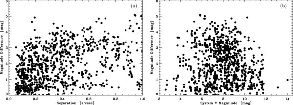
Figure 1. (a) Magnitude difference as a function of separation for the measures listed in Table 2. While a handful of separation measures above 1 arcsec appear there, the plot has been truncated in order to clearly show the behavior at subarcsecond separations. (b) Magnitude difference as a function of system V magnitude for the measures listed in Table 2.
Download figure:
Standard image High-resolution image2.1. Pixel Scale and Orientation
In the present work, we have continued our practice of determining the pixel scale by observing bright unresolved stars with a slit mask attached to the tertiary mirror baffle support structure of the telescope. The data obtained through the mask exhibit fringe patterns of separation that can be determined from the separation of the slits, the distance from the mask to the image plane, the telescope f/ratio, and the color of the light detected. As no changes in the telescope configuration have been made since the publication of our last set of measures, we used the same figures for all but the last parameter, namely the color of light detected. While we do use narrow bandpass filters with well-determined center wavelengths as described in Meyer et al. (2006), the color of the star can also have a small effect on the effective center wavelength. We accounted for this by using the spectral library of Pickles (1998) to estimate the spectral energy distribution for a star of the same type as that of the target. By combining the filter transmission curve with the atmospheric transmission, detector quantum efficiency, and the spectral energy distribution, we obtain a function that is an estimate of the light detected as a function of wavelength. The centroid of this function is determined in order to deduce the true effective center wavelength of the slit-mask observation. The scale values obtained showed a slight increase from run to run; this may be due to a small shift of one or more optical elements inside the speckle optics box over time. We chose therefore to apply the scale value obtained on each run to the data for that run. Although the uncertainty in the scale value varied from run to run, a mean uncertainty of about 0.1% was obtained, excluding two runs where the formal value was near zero. We judged these uncertainties to be unrealistically low; in these cases, we obtained good mask observations only in one filter and only on one star and so these uncertainties do not incorporate the uncertainty of the effective wavelength of the observation.
As in our past work, we determined the orientation of the pixel coordinate axes with the celestial coordinates by taking a series of short (typically 1 s) exposures of a bright star and offsetting the telescope in different directions from a home position by a small amount (typically 5 arcsec). This was normally done without autoguiding, so that small drifts in position were possible from the start of the sequence to the end. Our analysis made use of the redundant home position images to estimate and remove any drift. This method actually gives both scale and orientation values, but we have found that the mask method gives significantly higher precision for the pixel scale than the offset method. After examining the individual orientation angles obtained, there was no evidence for a change from run to run, so the results from all six runs were averaged to produce a final number applied to all data presented. Table 1 shows a summary of the calibration results obtained on each run.
Table 1. Scale and Orientation for Each Run
| Dates of the Run | Scale (mas/pixel) | Orientation Angle |
|---|---|---|
| 2007 Jan 2–5 | 29.530a | +0.213 ± 0.155 |
| 2007 Apr 28–30, May 1 | 29.730 ± 0.008 | +0.213 ± 0.155 |
| 2007 Jun 2–5 | 29.910 ± 0.004 | +0.213 ± 0.155 |
| 2007 Oct 26–29 | 29.920 ± 0.022 | +0.213 ± 0.155 |
| 2008 Jan 26 | 29.960a | +0.213 ± 0.155 |
| 2008 Jun 17–19 | 29.902 ± 0.064 | +0.213 ± 0.155 |
Note. aThe formal standard error associated with these measures was very close to zero as all observations analyzed gave nearly the same scale value.
Download table as: ASCIITypeset image
2.2. Reduction Method
Little about our reduction scheme has changed since our last large set of data was published in this series (Horch et al. 2008, Paper V). As described there and in previous papers, we performed a weighted least-squares fit to the average spatial frequency power spectrum of the speckle data frames, after this power spectrum had been divided by an unresolved source from The Bright Star Catalogue (Hoffleit & Jaschek 1982). This leaves the pure (deconvolved) fringe pattern, where the spacing of the fringes, their orientation, and the depth of fringe minima can be related to the separation, position angle, and magnitude difference of the system, respectively.
Two minor changes have been made, however. In the past, we determined the quadrant of the secondary from a reconstructed image made with two low-order subplanes of the bispectrum and the power spectrum. In this data set, we experimented with the use of several more bispectral subplanes, and found that this led to a somewhat more robust determination of the quadrant. This results in fewer "ambiguous" quadrant determinations in this work compared to our previous papers in the series. A second necessary adjustment was to incorporate the gain (in electrons per ADU) and read noise appropriate for the PIXIS CCD, so that the weights obtained for the fitting procedure reflected as best as possible the true signal-to-noise ratio (SNR) in the power spectrum.
3. RESULTS
Table 2 contains our main body of results. The column headings give (1) the Washington Double Star (WDS) number (Mason et al. 2001), which also gives the right ascension and declination for the object in 2000.0 coordinates; (2) the Bright Star Catalogue (i.e., Harvard Revised (HR)), Aitken Double Star (ADS), Durchmusterung (DM), or Gliese-Jahreiß (GJ) number of the object; (3) the Discoverer Designation; (4) the Henry Draper Catalogue (HD) number; (5) the Hipparcos Catalogue number; (6) the Besselian date of the observation; (7) the position angle (θ) of the secondary star relative to the primary, with north through east defining the positive sense of θ; (8) the separation of the two stars (ρ), in arcseconds; (9) the magnitude difference of the pair (Δm); (10) the center wavelength of the filter used for the observation (in nanometers); and (11) the full-width at half maximum (FWHM) of the filter transmission (in nanometers). In some cases, no magnitude difference measure is presented; this is due to the quality cut used for the photometry and described below in Section 3.2. Position angles have not been processed, and are therefore appropriate for the epoch of the observation shown.
Table 2. Double Star Speckle Measures
| WDS | HR, ADS | Discoverer | HD | HIP | Date | θ | ρ | Δm | λ | Δλ |
|---|---|---|---|---|---|---|---|---|---|---|
| (α,δ J2000.0) | DM, etc. | Designation | (2000+) | (°) | ('') | (nm) | (nm) | |||
| 00026 + 1841 | BD+17 5027 | HDS 2 | 225000 | 201 | 2007.8228 | 148.5 | 0.108 | 2.21 | 698 | 39 |
| 00061 + 0943 | BD+08 5172 | HDS 7 | 126 | 510 | 2007.0092 | 149.4 | 0.109 | 1.06 | 698 | 39 |
| 510 | 2007.0119 | 150.4 | 0.099 | 0.57 | 550 | 40 | ||||
| 510 | 2007.8173 | 162.2 | 0.119 | 0.24 | 754 | 44 | ||||
| 510 | 2007.8201 | 162.0 | 0.121 | 0.32 | 550 | 40 | ||||
| 510 | 2007.8255 | 161.9 | 0.121 | 0.31 | 550 | 40 | ||||
| 00062 − 0153 | BD−02 6098 | HDS 9 | 137 | 515 | 2007.8173 | 336.2 | 0.327 | 2.45 | 754 | 44 |
| 515 | 2007.8202 | 335.6 | 0.333 | 3.05 | 550 | 40 | ||||
| 00085 + 3456 | BD+34 3 | HDS 17 | 375 | 689 | 2007.8172 | 139.8 | 0.062 | 0.00 | 754 | 44a |
| 689 | 2007.8201 | 136.0 | 0.066 | 0.48 | 550 | 40a |
Notes. aQuadrant ambiguous, but consistent with previous measures listed in the 4th Interferometric Catalog. bQuadrant ambiguous, but inconsistent with previous measures listed in the 4th Interferometric Catalog. cQuadrant unambiguous, but inconsistent with previous measures listed in the 4th Interferometric Catalog.
Only a portion of this table is shown here to demonstrate its form and content. Machine-readable and Virtual Observatory (VO) versions of the full table are available.
Download table as: Machine-readable (MRT)Virtual Observatory (VOT)Typeset image
There are 53 objects in Table 2 that have not been previously resolved; we suggest discoverer designations of YSC "Yale-Southern Connecticut" 25–77, following the 17 objects with the same designation in Paper V and the 7 more (YSC 18–24) in Horch et al. (2009). Most of these objects were listed as "suspected double" in the Hipparcos Catalogue, though occasionally we have found a previously unreported component of a known binary or other bright star. Two hundred eighty nine objects in Table 2 were first reported in the Hipparcos Catalogue (these have discoverer designation HDS); of these, 187 have distances smaller than 100 pc, representing 65% of all HDSs in that distance range with separations below 2 arcsec and declination greater than −30°. (We do not generally observe systems with separations above 2 arcsec, as speckle offers little advantage over seeing limited observations in this case.) Forty-four of the HDS pairs have V > 10, meaning that these systems would not have been observable with the RIT CCD.
3.1. Astrometric Accuracy and Precision
We have studied the astrometric accuracy and precision of the measures in two ways: (1) by comparing our results with ephemeris predictions for objects with well-determined orbits, and (2) computing the relevant statistics for objects that we have observed three or more times on the same run. We detail the results of both studies below.
Since our observational program has shifted away from the "classic" speckle binaries in recent years, we have fewer observations of objects with the highest quality orbits to study than in the past. In order to obtain a sufficient sample of observations for statistical purposes, we have therefore relaxed the requirements on the quality of the orbits used somewhat from past work. We still considered only orbits of either Grade 1 or Grade 2 in the Sixth Catalogue of Orbits of Visual Binary Stars (Hartkopf et al. 2001a) which had stated uncertainties in the orbital elements, but we allowed the uncertainties in the ephemeris positions we calculated to be larger than in our previous work. To compensate for this somewhat, we also studied the trend of residuals from the orbit for the five most recent observations listed in the 4th Interferometric Catalog (Hartkopf et al. 2001b) and used this information as described below. Table 3 lists the objects and orbits used in this analysis.
Table 3. Orbits Used for the Measurement Precision Study
| WDS | Discoverer Designation | HIP | Coordinate(s) Used | Grade | Orbit Reference |
|---|---|---|---|---|---|
| 00121 + 5337 | BU 1026 | 981 | θ | 2 | Hartkopf et al. 1996 |
| 01072 + 3839 | A 1516 | 5249 | ρ | 2 | Hartkopf et al. 2000 |
| 01297 + 2250 | A 1910AB | 6966 | θ | 2 | Hartkopf et al. 1996 |
| 02262 + 3428 | HDS 318 | 11352 | ρ | 2 | Balega et al. 2005 |
| 04136 + 0743 | A 1938 | 19719 | θ,ρ | 1 | Hartkopf et al. 1996 |
| 04357 + 1010 | CHR 18Aa,Ab | 21402 | θ | 2 | Lane et al. 2007 |
| 06171 + 0957 | FIN 331Aa,Ab | 29850 | θ,ρ | 2 | Hartkopf et al. 1996 |
| 07277 + 2127 | MCA 30Aa,Ab | 36238 | θ | 2 | Mason 1997 |
| 07480 + 6018 | HU 1247 | 38052 | θ,ρ | 2 | Hartkopf et al. 1996 |
| 07518 − 1354 | BU 101 | 38382 | θ | 2 | Pourbaix 2000 |
| 07528 − 0526 | FIN 325 | 38474 | θ,ρ | 2 | Hartkopf et al. 1996 |
| 08468 + 0625 | SP 1AB | 43109 | θ,ρ | 1 | Hartkopf et al. 1996 |
| 09006 + 4147 | KUI 37AB | 44248 | θ,ρ | 1 | Hartkopf et al. 1996 |
| 09036 + 4709 | A 1585 | 44471 | θ | 2 | Barnaby et al. 2000 |
| 10083 + 3136 | KUI 48 | 49658 | θ,ρ | 2 | Hartkopf et al. 1996 |
| 10426 + 0335 | A 2768 | 52401 | θ,ρ | 2 | Hartkopf et al. 1989 |
| 12060 + 6842 | STF 3123AB | 59017 | θ | 2 | Hartkopf et al. 1996 |
| 12417 − 0127 | STF 1670AB | 61941 | θ,ρ | 2 | Scardia et al. 2007 |
| 13100 + 1732 | STF 1728AB | 64241 | θ,ρ | 1 | Mason et al. 2006 |
| 13396 + 1045 | BU 612AB | 66640 | θ,ρ | 1 | Mason et al. 1999a |
| 15232 + 3017 | STF 1937AB | 75312 | θ,ρ | 1 | Mason et al. 2006 |
| 17080 + 3556 | HU 1176AB | 83838 | θ,ρ | 1 | Hartkopf et al. 1989 |
| 17217 + 3958 | MCA 47 | 84949 | θ,ρ | 2 | Muterspaugh et al. 2008 |
| 17121 + 4540 | KUI 79AB | 84140 | ρ | 2 | Hartkopf et al. 1996 |
| 17372 + 2754 | KUI 83AB | 86221 | ρ | 2 | Mason et al. 1999a |
| 17490 + 3704 | COU 1145 | 87204 | θ,ρ | 2 | Hartkopf et al. 1996 |
| 17542 + 1108 | FIN 381 | 87655 | ρ | 2 | Hartkopf et al. 1996 |
| 18384 − 0312 | A 88AB | 91394 | θ,ρ | 1 | Hartkopf et al. 1989 |
| 19026 − 2953 | HDO 150AB | 93506 | θ | 1 | Mason et al. 1999a |
| 19598 − 0957 | HO 276 | 98416 | ρ | 2 | Pourbaix 2000 |
| 21135 + 1559 | HU 767 | 104771 | θ,ρ | 2 | Hartkopf et al. 1996 |
| 21145 + 1000 | STT 535AB | 104858 | θ,ρ | 1 | Muterspaugh et al. 2008 |
| 21446 + 2539 | BU 989 | 107354 | θ,ρ | 1 | Muterspaugh et al. 2008 |
| 21501 + 1717 | COU 14 | 107788 | θ | 2 | Hartkopf et al. 1989 |
| 22388 + 4419 | HO 295AB | 111805 | θ | 2 | Hartkopf et al. 1996 |
| 23052 − 0742 | A 417AB | 113996 | θ,ρ | 1 | Hartkopf et al. 1996 |
Download table as: ASCIITypeset image
Figure 2 shows the main result. In Figure 2(a), the observed minus ephemeris residuals in position angle are plotted as a function of separation while in Figure 2(b), a similar plot is presented for separation residuals. There are two subsamples for each plot. For position angle, open circles represent cases where the ephemeris uncertainty is less than 4°, and filled circles are cases where both the recent residual trend and the ephemeris uncertainty are less than 2 0. For separation, open circles are systems with ephemeris uncertainties of less than 5 mas, while filled circles have ephemeris uncertainties and residual trends of less than 3 mas. Both subsamples give average residuals very near zero, and the standard deviation of the residuals in the latter case is 2.92 ± 0.50 mas. Although some small portion of this dispersion is no doubt due to the orbital uncertainties, it nonetheless gives an approximate upper limit for the measurement precision of the data set. The measurement precision in position angle is inversely related to the separation of the system, since the linear measurement uncertainty corresponds to a larger angle at small separation. We have used the figure of 2.92 mas to estimate the position angle uncertainty expected as a function of θ, and we find that the data plotted in Figure 1(a) are consistent with this value.

Figure 2. (a) Residuals in position angle when comparing measures in Table 2 with the predicted position angle in the case of orbits of Grade 1 or 2. Open circles are orbits with predicted uncertainties <40 and filled circles are those with predicted uncertainties <20 that also have the average residual of the last five measures in the 4th Interferometric Catalogue <20. The dotted curves indicate the expected uncertainty in θ given a linear measurement uncertainty of 2.92 mas. (b) Residuals in separation when comparing measures in Table 2 with the predicted separation in the case of orbits of Grade 1 and 2. Open circles are orbits with predicted uncertainties <5.0 mas and filled circles are those with predicted uncertainties <3.0 mas that also have the average residual of the last five measures in the 4th Interferometric Catalogue <3.0 mas. The dotted lines indicate the offsets in separation residuals that would be generated by ±1σ errors in the typical scale determination as shown in Table 1. In both plots, the gray band at the left marks the region below the diffraction limit at 550 nm and the error bars indicate the predicted uncertainties derived from the uncertainties of the published orbital elements.
Download figure:
Standard image High-resolution imageWe also studied cases where we obtained three or more measures of the same system within a few days of one another (over which time it can be assumed that no orbital motion would be detected). As with the orbit study, we have fewer systems of this type here than presented in previous papers, but we find that the average standard deviation in these cases is 3.39 ± 0.71 mas in separation, indistinguishable within the errors from the orbit study result. In Figures 3(a) and (b), we plot the standard deviation in position angle and separation, respectively, obtained on these objects. In Figure 4, we plot the standard deviation in separation as a function of both total (system) V magnitude, and as a function of ΔHp, the magnitude difference appearing in the Hipparcos Catalogue. (Some systems did not have a ΔHp listed, so this plot has fewer points.) We can see particularly in the plot of σ(ρ) versus total magnitude that there is a trend toward higher values of the standard deviation at fainter magnitudes. This is to be expected as the SNR of the observation decreases. Table 4 summarizes the results of the astrometric precision studies. The results of the two studies are consistent, and these results are generally consistent with our previous work.
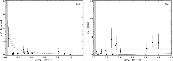
Figure 3. (a) Standard deviation of the position angle determination for objects observed three or more times. The dashed line is 0.17/ρ, where ρ is in arcseconds, which is the function expected for a linear measurement precision of 2.92 mas, the figure obtained in the speckle orbit study. The dotted curve is 0.19/ρ, which is the function expected for a linear measurement precision of 3.39 mas, the value obtained from multiple observations of the same targets. (b) Standard deviation of the separation determination for object observed three or more times. The dashed line is drawn at 2.92 mas, the figure obtained from the speckle orbit study, and the dotted line is drawn at 3.39 mas, the value from the study of multiple measures of the same targets. The solid line indicates the offset that would be produced by a 1σ error in the scale determination. In both plots, the gray band at the left marks the region below the diffraction limit at 550 nm.
Download figure:
Standard image High-resolution image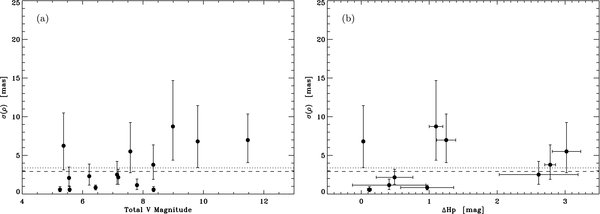
Figure 4. (a) Standard deviation of the separation determination for objects observed three or more times as a function of the total (system) V magnitude as it appears in the Hipparcos Catalogue. (b) Standard deviation of the separation determination for objects observed three or more times as a function of magnitude difference. In both plots, the dashed line is drawn at 2.92 mas, the value obtained from the speckle orbit study, and the dotted line is drawn at 3.39 mas, the value obtained from repeat observations of the same targets.
Download figure:
Standard image High-resolution imageTable 4. Astrometric Measurement Precision
| Object Type | Parameter | Average Residual | rms Deviation from Average Residual | Number of Measures |
|---|---|---|---|---|
| Orbits with δρ < 5.0 mas | ρ | −0.99 ± 0.71 mas | 4.11 ± 0.50 mas | 34 |
| Orbits with δρ and res. trenda <3.0 mas | ρ | −0.61 ± 0.71 mas | 2.92 ± 0.50 mas | 17 |
| Multiple Measures | ρ | ... | 3.39 ± 0.71 mas | 15 |
| Orbits with δθ < 40 |
θ | −0.18 ± 018 |
1.48 ± 013 |
69 |
| Orbits with δθ and res. trenda <20 |
θ | −0.05 ± 012 |
0.83 ± 009 |
45 |
| Multiple Measures | θ | ... | 0.65 ± 022 |
15 |
Note. aIn this study, the residual trend is defined as the mean residual of the last five measures appearing in the 4th Interferometric Catalog.
Download table as: ASCIITypeset image
3.2. Photometric Accuracy and Precision
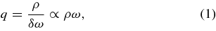
Our method of ensuring that the differential photometry obtained from the speckle observations is reliable is to estimate the degree of decorrelation between the speckle patterns of the primary and secondary stars. This depends linearly on the separation of the two stars and inversely on the size of the isoplanatic angle, as discussed in our previous papers, e.g., Paper V. In turn, the size of the isoplanatic angle is inversely related to the seeing itself, so that
where ρ is the separation of the two stars in arcseconds, δω is the size of the isoplanatic angle, and ω is the seeing. Defining q' = ρω in arcseconds squared, we can then plot the difference between the observed magnitude difference from our observations minus the magnitude difference appearing in the Hipparcos Catalogue as a function of q'. This is shown in Figure 5. We plot only objects that are near the main sequence in terms of their system magnitude and color; we require that the object have no flags for variability and that the Hipparcos magnitude difference has an uncertainty of less than 0.5 mag as shown in the Hipparcos Catalogue. Figure 5 shows a slight trend toward positive residuals as the q' becomes larger. This is expected, since the signature of decorrelation is a larger observed magnitude difference, leading to a larger observed residual in magnitude difference in this plot.

Figure 5. Observed magnitude difference minus ΔHp as a function of seeing times separation. Filled circles are measures taken in the 550 nm filter, and open circles are measures taken in the 698 and 754 nm filters.
Download figure:
Standard image High-resolution imageIn previous papers, we chose to only present a magnitude difference measure if an observation had a q' value of less than 0.6 arcsec2. In the case of Figure 5 presented here, it might be possible to argue for extending this to a slightly larger value since the function appears to remain relatively flat, but we would prefer to study this situation further before changing the cutoff value for two main reasons. First, there may be a color dependence to the cutoff value that could lead to a systematic error if not properly accounted for, and second, our ultimate goal is a proper understanding of the curve that would allow for a calibration of magnitude difference to be determined even in the case of high q' values. Therefore, in order to minimize any decorrelation error in our data and in order to be consistent with previous work, magnitude differences only appear in Table 2 if the observation has q' < 0.6 arcsec2.
With the collection of magnitude differences remaining after making this cut (leaving 809 of the 974 observations), it is then possible to study the photometric data quality further. Figure 6 shows the magnitude difference obtained in our study versus that appearing in the Hipparcos Catalogue, again excluding systems not near the main sequence, those with a variability flag in the catalog, and those with δ(ΔHp)>1.0. In our observations, three different filters were used, all redder and much narrower than that used in the Hipparcos observations; however, the bluest of the three filters, 550 nm, has a center wavelength most comparable to that of the Hp filter, and so in Figure 6 only the observations in the 550 filter are plotted. Using these data, we can compute the mean difference and standard deviation for various subsamples of data; these are listed in Table 5.

Figure 6. Observed magnitude difference vs. ΔHp for observations with seeing times separation less than 0.6 arcsec2. Only speckle data in the V and 550 nm filters are plotted. Open circles are measures with uncertainties in ΔHp ⩾ 0.10 mag, and filled circles are measures with uncertainties in ΔHp < 0.10 mag. The dashed line marks the line y = x.
Download figure:
Standard image High-resolution imageTable 5. Δm − ΔHp Results
| ΔHp Range | Average Residual | rms Deviation from | δ(ΔHp) | Number of |
|---|---|---|---|---|
| Average Residual | Measures | |||
| 0–1 mag | +0.18 ± 0.04 | 0.34 ± 0.03 | <1.00 | 76 |
| 1–2 mag | +0.07 ± 0.03 | 0.25 ± 0.02 | <1.00 | 55 |
| 2–3 mag | +0.13 ± 0.03 | 0.20 ± 0.02 | <1.00 | 50 |
| 3–4 mag | +0.12 ± 0.05 | 0.25 ± 0.03 | <1.00 | 28 |
| 4–5 mag | +0.14 ± 0.13 | 0.26 ± 0.09 | <1.00 | 4 |
| All | +0.13 ± 0.02 | 0.27 ± 0.01 | <1.00 | 147 |
| 0–1 mag | +0.18 ± 0.04 | 0.19 ± 0.03 | <0.10 | 26 |
| 1–2 mag | +0.06 ± 0.04 | 0.14 ± 0.03 | <0.10 | 12 |
| 2–3 mag | +0.08 ± 0.04 | 0.16 ± 0.03 | <0.10 | 14 |
| 3–4 mag | +0.02 ± 0.04 | 0.11 ± 0.03 | <0.10 | 8 |
| All | +0.11 ± 0.02 | 0.17 ± 0.02 | <0.10 | 60 |
Download table as: ASCIITypeset image
In previous papers, we have noted a slight positive trend to the Δm − ΔHp residuals, but argued that this is mainly due to the systems of small magnitude difference. Since a "negative" magnitude difference is usually reported as a positive number with a flip of the quadrant, there is a bias toward too large an average value in magnitude difference if the distribution of random errors crosses the zero-magnitude difference boundary. We can see that effect in the values shown in Table 5, where the average residual in the 0–1 mag bin is the largest. However, that does not completely explain the offset with the current data set, which extends to all magnitude differences at the level of a few hundredths of a magnitude. Combining the data of this paper and of Horch et al. (2008), which represents eight years of data with the same filter system, we see that there is evidence for an offset in the range of perhaps 0.02–0.06 mag for 1 < Δm < 4, with higher values obtained in the current work. The most likely explanation for this offset is color dependence of the quantity Δm − ΔHp. For example, in the current data, if we study the systems having δ(ΔHp) < 0.1 and 1 < ΔHp < 4, then the average value of this residual for systems with B − V < 0.6 is 0.04 ± 0.03, whereas for B − V > 0.6 it is 0.11 ± 0.03. The fact that the results presented in this paper have a larger offset than in Paper V can be explained by noting that the overall collection of objects is redder (with mean B − V color of 0.53 in the current data set versus 0.40 in Paper V), which is in turn due mainly to focusing here on fainter systems. In addition, information in Volume 1 of the Hipparcos and Tycho Catalogues (ESA 1997) concerning the definition and calibration of the Hp filter (specifically, Tables 1.3.5 and 1.3.6) suggests that a color effect in magnitude difference of order 0.1 mag exists between Hp and the Johnson V filter. It is not unreasonable to suppose that a similar effect exists between Hp and our 550 nm filter, which has not been seen clearly in previous papers because the distribution of colors for objects observed were bluer than the current data set. Obviously, this situation warrants further study, and its resolution will be needed to fully understand the systematics of our speckle photometry at the level of a few hundredths of a magnitude. Nonetheless, Figure 6 shows unequivocally that good photometric information is retained in the speckle data.
Turning now to the rms deviations from the average residuals (Column 3 of Table 5), in general these values are larger when the sample includes ΔHp values of larger uncertainty. This is expected, since the rms deviation will have statistically independent contributions from the uncertainties in the speckle data as well as those of Hipparcos which should in theory add in quadrature. In the case of sample with δ(ΔHp) < 1.00, the average value for δ(ΔHp) is 0.27 mag, whereas it is 0.052 mag for the subsample with δ(ΔHp) < 0.10. In the latter case, we may therefore roughly conclude that the values in Table 5 for the rms residuals represent an upper limit in our photometric precision, since the contribution of the Hipparcos uncertainty in this case, though present, will be relatively small. Thus, our photometry should have precision no worse than the range 0.1–0.15 mag in general.
There are a small number of cases of objects in Table 2 where we have three or more magnitude difference measures in the same filter. This allows us to study the repeatability of the photometry. These results are shown in Figure 7 and Table 6. In our past work, we modeled the uncertainty in our magnitude difference measures in terms of the SNR in the spatial frequency power spectrum. Due to factors such as seeing and the magnitude of the source, systems with a given magnitude difference can have a range of signal-to-noise ratios under typical observing conditions. In Figure 7, we have plotted high, low, and average cases of signal-to-noise at WIYN from our previous work. We find that, although we do not have many cases to compare to in the current data, they are nonetheless consistent with previous results. Likewise, in Table 6, the data overall indicate a typical uncertainty of 0.10 mag per observation.

Figure 7. Standard deviation in Δm as a function of average Δm for objects observed three or more times in one filter. The heavy solid line is the best-fit curve based on SNR as described in Paper V, and the dotted curves are parameterized curves for high and low values of the SNR observed at WIYN. The large filled circles are average values of σ(Δm) for the open circles clustered nearby.
Download figure:
Standard image High-resolution imageTable 6. Δm Repeatability Results
| Δm | rms Deviation from | Number of |
|---|---|---|
| Average | Average Value (σ) | Measures |
| 0.31 | 0.111 ± 0.031 | 3 |
| 1.15 | 0.079 ± 0.032 | 2 |
| 2.93 | 0.072 ± 0.036 | 3 |
| All | 0.088 ± 0.018 | 8 |
Download table as: ASCIITypeset image
It may seem contradictory that, with a much better detector than in previous work, we obtain comparable results in terms of both astrometric and photometric precisions. However, this is expected because the (SNR) per frame in speckle interferometry is constant in the relatively photon-rich regime, essentially a limit imposed by the atmosphere. As the target becomes fainter, the detector read noise and quantum efficiency do limit the SNR of the observation, and indeed the SNR falls off dramatically at that point, especially for CCDs, as discussed in Horch et al. (1997). With a better detector, the theoretical SNR curve is merely shifted to fainter magnitudes, but remains relatively flat until the cutoff is reached. Thus, no significant gains in precision are realized.
3.3. Orbit Determinations
When the above measures are combined with the list of existing observations in the 4th Interferometric Catalog, several objects exhibit motion sufficient for either orbit redetermination or the first determination of orbital parameters. We limit the discussion to the six most obvious cases, two of which lead to orbit revision and the other four to preliminary orbits. To calculate the orbits discussed below, we have used the code of MacKnight & Horch (2004), and we have only used data from the 4th Catalog. We have estimated uncertainties in the orbital parameters by assuming 3 mas linear uncertainties in the individual measures and adding Gaussian random deviates to the position angles and separations based on that assumption. In this way, we can calculate the orbit many times with different random deviates added in each case, and then compute the standard deviation in the collection of each orbital element obtained. We discuss first the orbit revisions below.
- 1.HDS 3083 (HIP 106972). The current orbit in the 6th Orbit Catalog is that of Balega et al. (2005), where the quadrant of the Hipparcos observation was assumed to be incorrect, and an orbit of period 18.57 ± 0.06 years was obtained for this system of composite spectral type M1.5 and modest magnitude difference. However, our observation of 2008.4641 has very large residuals from the ephemeris position. Computing a new orbit that includes the new astrometric data, we find the orbital elements shown in Table 7. This orbit requires no quadrant flip of the Hipparcos data point and shortens the orbital period to 11.7 years. This does raise the implied mass sum from 0.89 ± 0.25 solar masses (using the Balega et al. orbit) to 1.29 ± 0.41 solar masses (for our orbit) if the Hipparcos parallax is used, but either value is essentially consistent within the uncertainties with what one would expect in the case of two early M dwarfs. The two orbits are shown together in Figure 8.
- 2.HEI 88 (HIP 115279). In this case, the current orbit is due to Seymour et al. (2002). However, two recent observations reported in Horch et al. (2008) are significantly off the orbital trend. Quadrant determinations for these observations are also difficult to understand in the context of the Seymour et al. orbit, as one which was not ambiguous appeared to be incorrectly determined, and the second observation had a quadrant determination that was reported as ambiguous but was apparently consistent with previous data. Our 2007 observation from Table 2 is also unambiguous in terms of the quadrant, but again inconsistent with the Seymour orbit. Our orbital parameters for this system, calculated with the new data, are shown in Table 7. The two orbits are shown side-by-side in Figure 9. In our orbit, the only point which requires a quadrant flip is the point labeled ambiguous in Horch et al. (2008). Both the period and semi-major axis are reduced from the Seymour et al. values, and the mass sum is reduced from two solar masses to 1.57 ± 0.55. This system also has a modest magnitude difference, so that one might worry about this decrease in the mass for a late-F system on the main sequence. However, the Geneva-Copenhagen spectroscopic survey of the solar neighborhood (Nordström et al. 2004) lists the metallicity for HEI 88 as −0.39, significantly metal poor. The mass sum for a given spectral type will be decreased in the metal poor case, so that, given the uncertainties, our mass sum is not unreasonable at this stage.
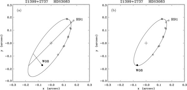
Figure 8. (a) Orbital data for the binary HDS 3083 = HIP 106972. The orbit plotted is that of Balega et al. (2005). (b) The same data plotted with a revised orbit based in part on the data appearing in Table 2. In both plots, the plus symbol marks the location of the primary, open circles are points appearing in the 4th Interferometric Catalog, filled circles are points appearing in Table 2, and line segments are drawn from the ephemeris prediction to the observed location of the secondary in each case. "H91" indicates the Hipparcos measure, and "W08" indicates a WIYN measurement with "08" corresponding to the year of the observation (2008).
Download figure:
Standard image High-resolution image
Figure 9. (a) Orbital data for the binary HEI 88 = HIP 115279. The orbit plotted is that of Seymour et al. (2002). (b) The same data plotted with a revised orbit based in part on the data appearing in Table 2. In both plots, the plus symbol marks the location of the primary, open circles are points appearing in the 4th Interferometric Catalog, filled circles are points appearing in Table 2, and line segments are drawn from the ephemeris prediction to the observed location of the secondary in each case. "H91" indicates the Hipparcos measure, and "W07" indicates the WIYN measurement appearing in Table 2 from 2007. In our orbit, one measure has the quadrant reversed from the Seymour orbit; that measure has an ambiguous quadrant determination in Paper V.
Download figure:
Standard image High-resolution imageTable 7. Orbital Revisions for Two Systems
| Parameter | HDS 3083 | HEI 88 |
|---|---|---|
| P (years) | 11.73 ± 0.24 | 32.86 ± 0.50 |
| a (mas) | 0.224 ± 0.011 | 0.156 ± 0.001 |
| i (deg) | 71.7 ± 3.0 | 0.3 ± 3.1 |
| Ω (deg) | 147.9 ± 2.9 | 13.8 ± 8.0 |
| T0 (years) | 2006.26 ± 0.60 | 2003.02 ± 0.04 |
| e | 0.357 ± 0.035 | 0.617 ± 0.006 |
| ω (deg) | 106. ± 14. | 16.6 ± 7.8 |
Download table as: ASCIITypeset image
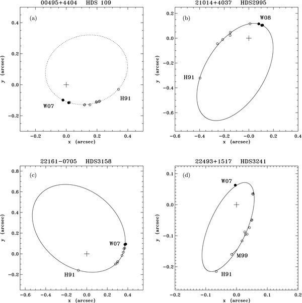
We have also determined preliminary orbits for four Hipparcos double stars. Orbital elements for these system appear in Table 8, and graphical representations of the orbit are shown in Figure 10. We discuss these briefly below.
- 1.HDS 109 (HIP 3857). Judging from the spectral type and magnitude difference appearing in the Hipparcos Catalogue (G0 and 2.30 ± 0.11, respectively), this system consists of a primary star near G0 with a companion of approximate spectral type K3, assuming the pair is on the main sequence. Nordström et al. (2004) state the metallicity to be very near solar. Thus, a guess of perhaps 1.75 solar masses for the mass sum based on this information is reasonable. So far we have seen the system only traverse about 90° in position angle since the discover observation, so the orbital elements are very uncertain at this stage. They imply a mass sum of 0.94 ± 0.38, lower than expected. While it is nearly certain that this orbit will need revision eventually, the orbital elements here should provide adequate ephemerides for observers over the next decade.
- 2.HDS 2995 (HIP 103749). Orbital data span approximately 180° for this system, with decreasing separation since the discovery observation. However, the system passed through periastron in 2007, and observed separations should begin to increase over the next few years. With spectral type F5 and magnitude difference of 3.37 ± 0.09 according to the Hipparcos Catalogue, one would expect roughly an F4-F5 primary with a K4 secondary, yielding a mass sum of approximately 2 solar masses for a system of solar metallicity. The mass sum implied from our orbital elements is 1.45 ± 0.19 solar masses, but like HEI 88 discussed above, this is a metal poor system (with metallicity −0.21 in the Geneva-Copenhagen Catalogue), so a true value of below 2 solar masses is certainly possible.
- 3.HDS 3158 (HIP 109951). In this case, we have orbital data spanning 130° in position angle, which yield an orbit with a period of 134 years. The dynamical mass sum implied is 2.98 ± 0.91 solar masses, which appears to be too high to be consistent with the composite spectral type of G5 with a magnitude difference of approximately 2. These data would suggest a primary of perhaps G4 and a secondary of K4, leading to a mass sum of approximately 1.7 solar masses.
- 4.HDS 3241 (HIP 112695). It was necessary to flip the quadrant of the observations in the interval 2000.88 to 2004.84 in order to obtain the orbit shown in Figure 10(d) of this system. Most observations of the system to date have been made by Balega et al. (2002, 2006, 2007). Given the magnitude difference of over 2, it seems unlikely that a quadrant determination would be ambiguous or incorrect, but nonetheless there is a clear discontinuity in the position angle between 1999 and 2000 that is also equally unlikely. Our measure in Table 2 marks a second discontinuity in position angle, and the orbit obtained (after quadrant reversals) gives a period of 34 years. Because there is still a large uncertainty in the period, the dynamical mass sum obtained is still quite uncertain, 3.2 ± 1.9 solar masses. Nonetheless, it is consistent with what we could reasonably guess as the spectral types of the components, say G5 and K5, leading to perhaps 1.7 solar masses.
Figure 10. Orbital data for four binaries discussed in the text. (a) HDS 109. Here we draw the orbit with a dotted line to indicate the relative uncertainty of this calculation. (b) HDS 2995. (c) HDS 3158. (d) HDS 3241. In all plots, "H91" indicates the Hipparcos measure, and "WXX" indicates a WIYN measurement with XX corresponding to the year of the observation. In (a), "M99" corresponds to a measure by Mason et al. (1999b), where the authors state that the measure is of reduced quality.
Download figure:
Standard image High-resolution image
Table 8. Preliminary Orbital Elements for Four HDS Systems
| Parameter | HDS 109 | HDS 2995 | HDS 3158 | HDS 3241 |
|---|---|---|---|---|
| P (years) | 97. ± 10. | 97.68 ± 0.64 | 134.0 ± 1.4 | 34.4 ± 6.6 |
| a (mas) | 0.307 ± 0.022 | 0.464 ± 0.004 | 0.567 ± 0.007 | 0.156 ± 0.006 |
| i (deg) | 144.4 ± 8.4 | 133.05 ± 0.89 | 45.3 ± 2.2 | 63.5 ± 4.8 |
| Ω (deg) | 246.0 ± 5.0 | 313.0 ± 3.1 | 248.7 ± 3.6 | 153.8 ± 2.1 |
| T0 (years) | 2009.57 ± 0.22 | 2007.25 ± 0.64 | 2128.0 ± 1.3 | 2006.76 ± 0.56 |
| e | 0.626 ± 0.059 | 0.695 ± 0.006 | 0.580 ± 0.014 | 0.502 ± 0.031 |
| ω (deg) | 295. ± 11. | 146.3 ± 4.9 | 119.5 ± 1.2 | 12. ± 15. |
Download table as: ASCIITypeset image
4. CONCLUSIONS
We have presented 974 speckle observations of binary stars taken at the WIYN 3.5 m Telescope. Astrometric and photometric quality of these observations appears consistent with our previous work, namely linear measurement precision of approximately 3 mas, and photometric precision of approximately 0.1 mag per observation. A slight offset between magnitude differences obtained here in the 550 nm filter and those in the Hipparcos Catalogue exists on the level of ∼0.05 mag, judging from well-determined ΔHp values. Further work will be needed to conclusively determine the source of this offset, but current evidence suggests that it is related to the color of the source. Orbit redeterminations have been suggested for two systems, and orbital elements have been obtained for the first time for four other systems. While these orbits are not yet high enough in quality to use the implied dynamical mass sums in astrophysical studies, it is clear that these systems merit future observations for that purpose.
We thank George Will, Charles Corson, Doug Williams, Karen Butler, and Dave Summers for their assistance at the telescope. This work was funded by NSF grants AST-0307450 and AST-0504010, and AST-0908125. It made use of the Washington Double Star Catalog maintained at the U.S. Naval Observatory and the SIMBAD database, operated at CDS, Strasbourg, France.
Footnotes
- *
The WIYN Observatory is a joint facility of the University of Wisconsin-Madison, Indiana University, Yale University, and the National Optical Astronomy Observatories.