
ABSTRACT
The future direct imaging of exoplanets depends critically on wave-front corrections. Extreme adaptive optics is being proposed to meet such a critical requirement. One limitation to the performance of adaptive optics is the differential wave-front aberration that is not measured by a conventional wave-front sensor because of the so-called non–common-path error. In this article, we propose a simple approach that can be used to eliminate differential aberration with extreme adaptive optics and is optimized for best image performance or directly optimized for high-contrast coronagraphic imaging. The approach that we propose can correct differential aberration in a single step, which guarantees high accuracy and allows adaptive optics to correct the differential aberration on a real-time scale. This approach is based on an iterative optimization algorithm that commands the deformable mirror directly and uses the focal-plane point-spread function as a metric function to evaluate the correction performance.
Export citation and abstract BibTeX RIS
1. INTRODUCTION
With more than 700 exoplanets known to date, it is clear that exoplanets are common. Most exoplanets have been discovered with radial velocity and transiting techniques, which are both indirect detection methods. A few have been found with direct imaging. Future direct imaging discoveries of exoplanets will be one of the most important scientific advances in astronomy. It is generally agreed that the characterization and detailed study of an exoplanet require direct imaging. Direct detections of exoplanets remain challenging, since exoplanets are very faint, compared with their nearby parent stars. In theory, a high-contrast coronagraph can be used to suppress the star's diffracted light, so that the exoplanet can be detected. For imaging of Jupiter-like exoplanets in the visible, a contrast of 10-8–10-9 is required, and no ground-based instrument can currently achieve such performance. The actual performance of a ground-based coronagraph is seriously limited by the incoming wave-front aberrations that are induced by atmospheric turbulence. For such direct imaging, an extreme adaptive optics (AO) system is required (Baudoz et al. 2010).
For an AO-corrected point-spread function (PSF), the wave-front error-induced speckle noise will limit the performance for high-contrast imaging (Racine 1999). The current extreme adaptive optics systems will be optimized for ultimate system performance, which will be able to deliver a contrast on the order of 10-7 for coronagraphic imaging. The correction of non–common-path error is one of the critical issues for an extreme AO system (Fusco et al. 2006). Extreme adaptive optics systems are being developed for GEMINI, VLT, and Palomar 200 inch telescopes (Severson et al. 2006; Baudoz et al. 2010; Dekany et al. 2006). Studies for future exoplanet finder coronagraphs such as SPHERE/VLT or GPI/GEMINI show that one of the performance limitations is the differential wave-front error that is introduced by the so-called non–common-path error and is not measured by the AO wave-front sensor, which is physically separated from the wave-front sensor and the science camera (Baudoz et al. 2010). Such a residual static and quasi-static wave-front error limits the contrast of coronagraphic imaging and must be effectively eliminated before an extreme AO system can be fully functional (Sivaramakrishnan et al. 2002; Macintosh et al. 2006; Sivaramakrishnan et al. 2008).
Different approaches were proposed to measure the differential wave-front error, and the wave-front measurement data are subsequently used to characterize the AO system or remove the differential aberration. Phase diversity algorithms are used to measure the differential wave-front aberration (Sauvage et al. 2007; van Dam et al. 2004; Hartung et al. 2003; Rousset et al. 2002), which involves an estimation for both amplitude and phase. The phase-diversity approach is being used for the extreme AO system for the Spectro-Polarimetric High-contrast Exoplanet REsearch (SPHERE) with the VLT (Fusco et al. 2006; Sauvage et al. 2007). Recently, dedicated interferometers have been proposed that can deliver high-precision measurement. The Palomar Hale Telescope high-contrast imaging program uses a postcoronagraph calibration interferometer to measure the differential aberration (Hinkley et al. 2011). To achieve high measurement accuracy, the Gemini Planet Imager (GPI) system uses a phase-shifting interferometer (Wallace et al. 2010). The measurement accuracy required for these interferometer approaches is on the order of a few to 10 nm (Hinkley et al. 2011; Wallace et al. 2010). Although successfully demonstrated, such a requirement is still challenging, and a dedicated interferometer is required to achieve such a goal.
All of the preceding approaches require two steps: The first step is for the measurement of the wave-front error only, such as using an interferometer or the phase-diversity algorithm, in which only pure wave-front measurement is conducted and no deformable mirror wave-front correction is involved. The second step is the wave-front correction that is based on the information from the measured wave front. The performance of the two-step approach is limited by a number of factors (Sauvage et al. 2007; Hartung et al. 2003; Blanc et al. 2003), since errors may be introduced in this process, which will be added into the AO in step 2. Therefore, the measurement precision required is extremely high. Also, the deformable mirror may not be able to exactly reproduce the measured wave front that will be corrected, or the measurement performance might be limited by the number of terms/orders of Zernike polynomials. The phase diversity for the VLT measured 15 orders of Zernike polynomials only (Hartung et al. 2003), and higher-order aberration information has been missed. A deformable mirror (DM) for extreme AO, in general, may have hundreds or thousands of actuators and will be able to reproduce much higher orders of Zernike polynomials. Most of these limitations are inherited from these two individual steps.
In this article, we present an alternative approach that can be used to remove the differential wave-front error. This is achieved by using a focal-plane PSF evaluation algorithm that directly commands the AO DM and is optimized for best imaging performance or directly optimized for high-contrast coronagraphic imaging, which results in direct correction of the differential aberration in a single step. The elimination of the pure wave-front measurement greatly simplifies the correction of the differential aberration and makes it easy to implement. For our approach, no dedicated interferometer is required, and for an existing AO, the only hardware required is a high-quality camera for PSF evaluation. In such a way, a conventional AO system can not only eliminate the differential wave-front error that an AO wave-front sensor cannot measure, but it can also provide high-quality imaging performance on a real-time scale. In addition, we will show that our one-step approach is more flexible and can also be used with an AO system with a Shark-Hartmann wave-front sensor (S-H WFS) to create a dark hole for high-contrast coronagraphic imaging. In § 2, we discussed the general principle of our algorithm. In § 3, we present our laboratory results. Conclusions are given in § 4.
2. PRINCIPLE
The schematic diagram of the system for the non–common-path error correction is shown in Figure 1. A single-mode fiber (SF) that can be inserted onto the telescope focal plane is used for the correction and calibration of the AO system, in which the light emitted from the fiber is served as a perfect point source. The fiber is only used for the calibration/correction and can be removed. The light is collimated by lens L1 and reflected by a tip-tilt mirror (TM), as well as a deformable mirror (DM) that can be commanded to correct possible wave-front error. A beam-splitter (BS) directs part of the incoming light to the S-H WFS, which consists of lenses L3 and L4, a microlens array (MLA), and a high-speed camera (C2). At the science-image focal plane, a science camera (C1) is used for PSF evaluation. The configuration of the hardware is a typical AO system, except for the fact that the science camera is used on the focal plane.
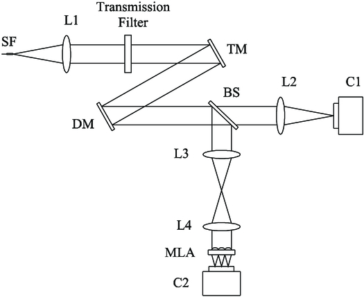
Fig. 1.— Schematic diagram of the SPGD differential wave-front correction and the AO system.
For a point-source image, a perfect PSF consists of a bright Airy disk surrounded by minimal diffraction fringes. If a wave-front aberration is presented, more intensity energy will be pushed into the diffraction fringes, reducing energy in the Airy disk. Therefore, the best PSF corresponds to an Airy pattern that has maximum energy in the bright Airy disk and has minimum energy in the diffraction fringes. For our direct focal-plane PSF evaluation and AO-correction algorithm, the goal is to find a minimum value for a system performance metric function J, by optimizing voltages applied on DM actuators. The metric function should be determined according to actual applications. For example, for best Strehl ratio, the metric function can be chosen as the relative energy in the diffraction fringes. For the correction of the static differential wave-front error, an iterative approach is acceptable, and we use the stochastic parallel gradient descent (SPGD; Vorontsov et al. 1997; Vorontsov & Sivokon 1998; Vorontsov & Yu, 2004) algorithm, which is an improved version of the well-known steepest-descent algorithm. It applies small random perturbations to all control parameters (voltages of actuators) simultaneously and then evaluates the gradient variation of metric function. SPGD is an iterative technique, which is applied for wave-front correction when the bandwidth is not a critical issue. Traditionally, since SPGD uses the focal-plane PSF for wave-front sensing, no S-H WFS is required for such an AO system that uses the SPGD technique (Vorontsov et al. 1997; Vorontsov & Sivokon 1998; Vorontsov & Yu, 2004). In fact, compared with a conventional AO system that uses an S-H wave-front sensor, a SPGD system can be viewed as the AO that has no wave-front sensor. The differential wave-front error can be compensated by optimizing the metric function that is calculated from the measured PSF on the focal plane. The control signals are updated in an iterative process using the following rule:

where k is the iteration number; u = {u1,u2,...,un} is the control signal vector (i.e., voltages applied on DM actuators); n is the control channel number (i.e., the actuator number); γ is the gain coefficient, which is positive for minimizing and negative for maximizing the metric function; δu denotes small random perturbations that have identical amplitudes and Bernoulli probability distribution; and ΔJ is the variation of the metric function:
To improve the estimation accuracy of δJ, a two-sided perturbation is used as

The gain coefficient γ adaptive to the metric function J is used to accelerate the convergence:

In our case, a point source is imaged onto the focal plane for PSF evaluation. Although other metric functions were used to evaluate imaging performances for a general system (Vorontsov 1997), for our specific applications, better metric functions exist. Considering an AO system with a goal to remove the differential wave-front error or to achieve best contrast in a local area (i.e., dark hole), we propose an improved metric function for the SPGD only, which has better performance for our applications and is optimized for minimum intensity energy in a specific area:
where Ii(x,y) is the focal-plane intensity in the PSF Airy disk that should have maximum value, while Io(x,y) is the intensity in an area around or near the Airy disk that should has minimum value. The metric function J is used to find the minimum value of sum Ii(x,y) relative to sum Io(x,y) in the defined areas. Figure 2 shows two possible applications of the algorithm. In Figure 2 (left), Ii(x,y) is the intensity defined in the Airy disk and Io(x,y) is the intensity defined in an annulus area (diffraction pattern) around the Airy disk. This can be used for optimization to remove the non–common-path error (i.e., maximum Strehl ratio). In Figure 2 (right), Ii(x,y) is still the intensity defined in the Airy disk, while Io(x,y) is the intensity defined in a located area nearby the Airy disk. This can be used to optimize for a local dark hole in an area defined by Io(x,y), which can provide an extra gain for high-contrast coronagraphic imaging.
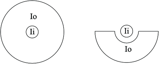
Fig. 2.— Definition of optimization area. Left: Optimized for minimum differential wave-front error. Right: Optimized for a local dark hole.
Please note that the algorithm defined by equation (5) has twofold results: (1) ensures a maximum energy in the Airy disk and (2) guarantees minimum energy in an area that is defined according to the specific application. These will be demonstrated with different examples in § 3.
For an AO system using S-H WFS, the slope vector is used for the wave-front measurement and wave-front correction by applying voltages on associated DM actuators. The slope vector ΔS is calculated as
where S is the centroid vector measured by S-H WFS in the AO-correction process, S = (x1,x2,...,xm,y1,y2,...,ym), m is the subaperture number of the S-H WFS, S0 = (xr,1,xr,2,...,xr,m,yr,1,yr,2,...,yr,m) is the centroid vector for the reference wave-front that is used for the AO calibration, xr,i and yr,i are the x and y coordinates of the number i subaperture for the reference wave front, and xi and yi are the x and y coordinates of the number i subaperture that are measured in the AO-correction process. When each component in the ΔS is zero, no voltage will be applied on the actuators. Therefore, the reference vector S0 determines what wave front will be viewed as perfect wave front by the AO system.
For an AO system using S-H WFS, the static non–common-path error is related with the reference vector S0, which is further associated with the reference wave front used for the AO calibration. Without the non-common-path correction, the WFS cannot see this error, so the AO cannot correct it. Once the PSF is corrected by the SPGD, DM voltages are locked and are used as the initial voltages for the AO calibration. In such a way, the reference wave front will be updated by the DM and the non–common-path error can be seen and corrected by the AO system. Although the SPGD is used for static or slow-variable wave-front correction, it has never been used to calibrate the non–common-path error for an AO system that uses a S-H WFS.
3. LABORATORY TEST
The schematic layout of the AO system for this test is shown in Figure 1. The wavelength for the test light source is 0.6328 µm. The DM we used for this test was purchased from the Boston Micromachines Corporation and has 140 actuators (12 × 12, excluding those in the four corners). Since the actuators at edges are restrained and cannot move freely, the DM has only 10 × 10–11 × 11 effective actuators. The tip-tilt system is based on a fast-tilting platform provided by Physik Instrumente. In this test, the tip-tilt mirror is not commanded. The WFS has a 13 × 13 lenslet (excluding those in the four corners), and Zernike polynomials up to 66 orders are used. The AO system used for this test is being used for high-resolution imaging with ground-based telescopes and was described in detail elsewhere (Ren et al. 2009, 2010, 2012).
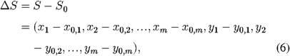
In our test, one DM actuator near the aperture center is defective or less active. The wave front can only be compensated by using its neighborhood actuators, which somewhat limits the DM performance. Figure 3 shows the PSF at different exposures delivered by the AO system, without the SPGD calibration. The left panel shows the PSF with proper exposure, and the right panel shows the same PSF with overexposure, in order to show details of the diffraction pattern. Since the AO WFS cannot see the differential wave-front error induced by the optical elements from the calibration single-mode fiber to the science camera, the PSF is somewhat aberrated, resulting in a low Strehl ratio. For the science camera, the transmission BS and L2 consist of the non–common path, while for the WFS, the reflective BS, L3, L4, and MLA belong to the non–common path. The differential error between these two cannot be seen by the WFS and thus cannot be corrected by the AO system. Compared with a perfect wave front with the differential aberration corrected, the rms wave-front error output from the WFS is 0.093 wavelengths, which corresponds a Strehl ratio of 0.71.
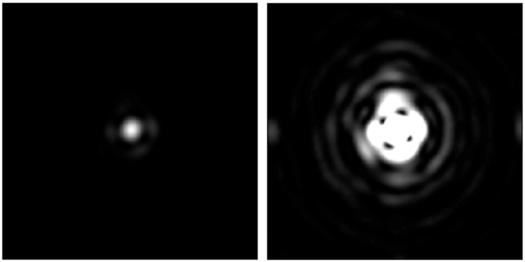
Fig. 3.— AO PSFs at different exposures without SPGD correction.
The aberrated PSF is corrected by using our SPGD algorithm. Figure 4 shows the PSF at different exposures directly corrected by the SPGD. In this optimization, Ii(x,y) is defined in the Airy disk, which has a radius up to 1.22λ/D, where λ is the wavelength of the test light source (0.6328 μm), and D is the effective aperture of the optical system. Io(x,y) is defined in an annulus area that has a radius between 1.22 ∼ 10λ/D, which is large enough to cover the remaining intensity energy, excluding the Airy disk (see Fig. 2, left). As a result of the SPGD correction, the PSF has a maximum enclosed energy in the Airy disk and a minimum energy in the remaining area. Since the image is good enough to be viewed as a perfect PSF, the SPGD-corrected wave front is defined as the perfect wave and is used as a reference wave front, which corresponds to a Strehl ratio of 1.0. Other wave-front errors are calculated in comparison with this wave front. Of course, the quality of the actual reference generated by the SPGD correction is determined mainly by the DM performance (i.e., how many actuators the DM has, which determines how accurately a wave front can be created), not by the SPGD algorithm.
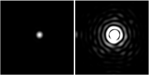
Fig. 4.— PSFs at different exposures achieved with the SPGD correction.
Once the best PSF is achieved on the focal plane, as shown in Figure 4, the DM voltages are locked. Now, the AO S-H WFS can see the updated reference wave front. The reference vector S0 is measured from the S-H WFS, is saved as a readable file, and will be used for future AO real-time correction. Subsequently, each time the AO is executed, it will automatically read and use the new reference vector S0, providing perfect correction on a real-time scale without further need of SPGD correction; the SPGD is only needed once during the AO calibration. Our AO system has a closed-loop bandwidth of ∼100 Hz, which provides real-time wave-front correction. Figure 5 shows the PSF at different exposures generated by the AO system, after the SPGD calibration. The rms residual wave-front error output from the corrected-AO WFS is 7.4 × 10⁻⁴ wavelengths, which defines the AO accuracy that can lock on a wave front corrected by the SPGD. Since the test system is located on a rigid optical table with an open surface in the air, the AO accuracy is determined by a number of factors, including the AO performance, vibration, and local air turbulence in the AO system. The 7.4 × 10⁻⁴ wavelength wave-front error corresponds to a Strehl ratio of ∼1.0. The PSF is almost totally identical to that in Figure 4 generated by the SPGD correction, indicating that the SPGD-created PSF is totally locked by the calibrated AO system.
Fig. 5.— PSFs at different exposures achieved with the adaptive optics calibrated by the SPGD algorithm.
The SPGD algorithm has the potentiality to allow a conventional S-H WFS AO system to create high-contrast imaging in a local dark hole on a real-time scale. The dark hole algorithm was originally proposed by Malbet et al. (1995) and was recently demonstrated by Trauger & Traub (2007), as well as by Give'On et al. (2007). Figure 6 shows the PSF of a dark hole generated by the SPGD algorithm. Again, Ii(x,y) is defined in the Airy disk with a radius up to 1.22λ/D, and Io(x,y) is defined as a rectangle with an small area of 1.5 × 4λ/D, but only including half of the PSF area (top half). In the local dark hole area, the intensity changes from 10-1.7 to 10-3.5, and an extra contrast gain of 65-times improvement has been achieved. Again, once the dark hole is generated by the SPGD, the DM voltages are locked. The new reference vector S0 is then recorded and saved as a readable file. The AO calibration is subsequently conducted. After the SPGD calibration, the AO is able to create a local dark hole on a real-time scale, no matter how the incoming wave front is changing. Figure 7 shows the PSF that is generated by the AO system with the updated reference vector S0. The PSF is again almost identical to that in Figure 6 directly generated by the SPGD, with an extra contrast gain of 65 times achieved in the dark hole. The AO system is able to lock on the SPGD-created wave front with a residual wave-front error of 2.98 × 10⁻⁴ wavelengths, which is consistent with the AO accuracy of 7.4 × 10⁻⁴ wavelength error. According to our knowledge, this is the first time that an AO S-H WFS is able to "see" and create a dark hole for possible high-contrast imaging.
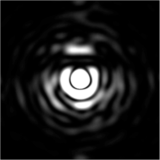
Fig. 6.— Dark hole image achieved with the SPGD algorithm.
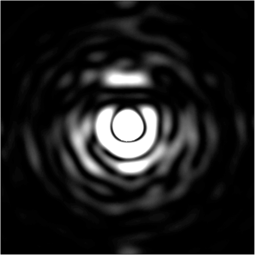
Fig. 7.— Dark hole image achieved with adaptive optics calibrated by the SPGD algorithm.
Please note that the dark hole test that we have conducted is a very initial result. In this test, further increasing the contrast in the dark hole is limited by a number of factors. The focal-plane camera is a commercial-grade camera that has a dynamic range of 14-bit digital depth and can only measure a contrast down to 10-4. No coronagraph is used in the system, which makes very high contrast extremely difficult or impossible. The small DM actuator number is a major limitation for the dark hole contrast. The edge actuators for the DM that we used are restrained, which further reduces the number of effective actuators. A calibrated transmission filter (Trauger & Traub 2007) that can reduce the image-plane Airy disk intensity so that the camera can measure a higher contrast is also needed.
The typical iteration number for the preceding tests is ∼300, which is determined from the metric function in each iteration. If the output metric function has no change or the change with each iteration is too small, no further iteration is needed and a solution is found. Figure 8 shows the evolution of a typical metric function during the SPGD optimization for the correction of the AO differential wave-front error. The running speed of the SPGD AO calibration is acceptable for our application. With a commercial Dell XPS 9100 personal computer equipped with an Intel i7 980 CPU, the AO calibration with the SPGD algorithm takes 3–5 minutes. The calibrations for both best Strehl ratio and the dark hole are only needed once, which is similar to the calibration of a conventional AO system. After the calibration, the reference vector S is saved. Therefore, after the SPGD calibration, our AO system can automatically lock on the new reference wave-front and provide a real-time correction up to 100 Hz bandwidth, which corresponds to ∼1000 open-loop corrections per second. Please note that the AO system that we discussed here is fundamentally different from the dark hole AO system discussed by Give'On et al. (2007), which has no S-H WFS and cannot provide real-time wave-front correction. The SPGD dark hole technique is also different from the conventional dark algorithm (Malbet 1995; Trauger & Traub 2007; Give'On et al. 2007). The conventional dark algorithm needs to know the DM influence function (Give'On et al. 2007), and the voltages applied on the DM are based on the solution of a first-order approximation equation. The SPGD does not need this information, and it automatically searches for the direction of gradient in the n-variable space that will be used for the next iteration, which makes the SPGD extremely simple and robust. The SPGD dark hole technique, however, is more time-consuming, which is not a problem for a "one-time" AO calibration.
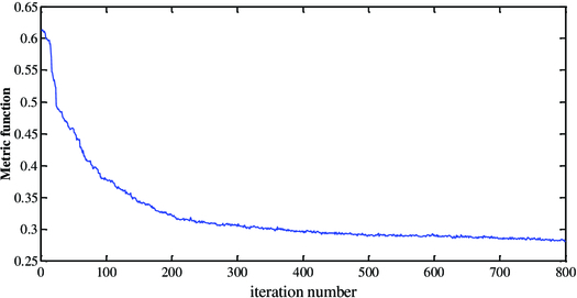
Fig. 8.— Evolution of metric function as a function of iteration number.
Since the physical relationship between the science-camera focal plane and the AO WFS is fixed, any wave-front variations upstream of the telescope focal plane can be seen by the SPGD-calibrated AO system and will thus be corrected on a real-time scale. These variations include the wave-front error induced by the telescope optics (which may change slowly), as well as that induced by the atmospheric turbulence (which may change rapidly).
4. CONCLUSIONS
We have shown that the SPGD algorithm can be used to directly command the AO DM and efficiently correct the non–common-path error, which can be used to find the perfect reference wave front for the AO calibration. After the SPGD calibration, the AO system can use its own S-H WFS automatically to correct the non–common-path error on a real-time scale. This approach is based on an iterative optimization algorithm that commands the AO DM directly, until the focal-plane PSF is fully corrected or a satisfactory result is achieved. Compared with other approaches, our approach involves only a single wave-front-correction step, and no extra wave-front measurement is required. The elimination of the wave-front measurement makes it simple and more accurate, and it will facilitate the implementation of extreme AO for high-contrast coronagraphic imaging. We showed that the SPGD-calibrated AO system can be optimized for best Strehl ratio and can lock on a wave front with accuracy on the order of 7.4 × 10⁻⁴ wavelengths. We also demonstrated that the SPGD calibration can allow an AO S-H WFS to lock on and create a dark hole for an extra contrast gain, with a wave-front lock accuracy of 2.98 × 10⁻⁴ wavelengths. In the experiment discussed in this article, no coronagraph is used. A potential application of the SPGD AO calibration is that it can be used with a coronagraph, and the AO system that deploys an S-H WFS can be calibrated for high-contrast imaging over the entire coronagraphic discovery area.
We thank the anonymous referee for valuable comments, which significantly improved the article. This work is supported by the National Science Foundation (grant ATM-0841440), the National Natural Science Foundation of China (grants 10873024 and 11003031), the National Astronomical Observatories' Special Fund for Astronomy-2009, and the Advanced Research of Space Science Missions and Payloads of the Space Science Strategic Pioneer Program, Chinese Academy of Sciences.