
ABSTRACT
On‐orbit data characteristics of the Space Telescope Imaging Spectrograph (STIS) CCD aboard the Hubble Space Telescope have been explored with early calibrations in a number of limiting conditions. At a gain of 4 e− DN−1, STIS CCD data show excellent linearity at high count levels, even for extreme oversaturation of individual central pixels. At low count levels we interpret a position‐ and intensity‐dependent nonlinearity in terms of charge transfer (in)efficiency in the parallel clocking direction and provide a simple model that accounts for this. A short time series of spectra was acquired at short‐exposure times and high signal‐to‐noise ratio (S/N) on the binary system α Cen A and B enabling the shutter repeatability to be quantified at 0.0002 s. A direct demonstration of near‐Poisson–limited time series with S/N>3000 is shown.
Export citation and abstract BibTeX RIS
1. INTRODUCTION
CCDs and their associated electronics are known to provide generally stable and linear response, but with various exceptions such as nonlinearities at low and/or high count levels. We present the results of exploratory on‐orbit calibrations of the Space Telescope Imaging Spectrograph (STIS) CCD on board the Hubble Space Telescope (HST) in limiting data regimes of both low and high exposure levels. Of particular interest are findings of (1) excellent high count level linearity when the gain = 4 e− DN−1 (electrons per data number) electronics are used even for count levels well beyond saturation, (2) a low count level nonlinearity probably resulting from imperfect charge‐transfer efficiency (CTE), and (3) excellent time series signal‐to‐noise (S/N) limits in excess of 3000 per exposure when using a spectroscopic mode to allow counting a sufficient number of e− from the source. Background information on the design of STIS in general and the CCD subsystem in particular can be found in Woodgate et al. (1998) and Kimble et al. (1994), respectively.
The observations used to investigate each data attribute will be referenced in sections devoted to individual topics. Most of the observations were obtained from the Cycle 7 STIS calibration program STIS/CAL‐7666 "CCD Linearity and Shutter Stability" which used three external target orbits and four internal calibration lamp occultation intervals. We will also refer to results from ground‐test data and use information regarding the operation of the CCD shutter mechanism in interpreting the results. In § 2 we discuss linearity at high count levels for gain = 4. The behavior at high count level for the 4 times fewer electrons per data number gain = 1 case is presented in § 3. Effects at low count level, including a detailed interpretation of CTE and an empirical model that can be used to linearize the data, are discussed in § 4. The exposure time repeatability is quantified in § 5 along with discussion of a technique for reaching S/N>3000 per exposure with expectations that S/N levels in excess of 10,000 can be reached with longer exposure times and collection of adequate charge. An overview of current results and open issues is provided in a closing discussion section.
2. HIGH COUNT LEVEL LINEARITY: GAIN 4
We adopted the general empirical approach of taking exposures at several levels from order 10% of full well depth, to (and even well beyond) saturation, and then simply comparing resultant count levels to establish the degree to which linearity is maintained. Data were acquired in three different modes: (1) A sparse field in M67 was imaged for which count levels ranged from well below to 50 times above saturation. (2) Simultaneous slitless, spectroscopic observations of α Cen A and B with the spectra separated by about 7 pixels in cross‐dispersion at exposure levels from well under to 5 times saturation. (3) Flat‐field internal calibration lamp exposures taken with an interleaved standard exposure to allow removal of possible drifts in lamp intensity, and covering 1/8 of full well to near saturation in 1/8 steps. Results from these tests were all consistent in showing that the STIS CCD has a nearly perfect linear response at gain = 4. A somewhat surprising result follows that both photometric and spectroscopic fidelity are maintained to well beyond saturation as long as the signal extraction algorithm counts electrons that have bled into adjacent pixels along columns.
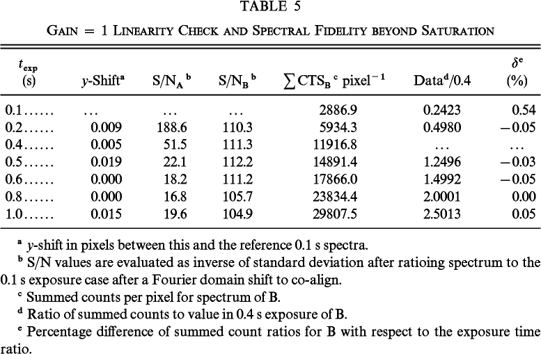
One orbit of Continuous Viewing Zone (CVZ) observations (obtained 1998 May 5) was devoted to simultaneous slitless spectroscopy of α Cen A and B to explore linearity at both gain = 1 and 4 and to provide a test of shutter stability and high S/N time series capability. Exposure times ranged from the minimum commandable value of 0.1 s for optical spectra to 180 s for a few UV exposures. A total of 36 spectra used the G430M grating at the central wavelength of 3423 Å for gain = 1, and 67 spectra used G430M, 5471 Å for gain = 4, with an order‐of‐magnitude spread in individual exposure times for each.
Table 1 provides the primary gain = 4 linearity results. The pipeline‐calibrated data with cosmic rays eliminated have simply been averaged over the primary pixel domain of x = 66–592, y = 2–19. The full 1024 range in x was not utilized; a subarray of 32 cross‐dispersion rows was specified, and inadequate subarray centering coupled with a sloping spectral order led to the (G430M, 5471 Å) spectrum of α Cen B touching the edge of the subarray for x≳600.
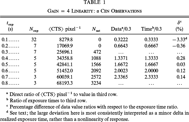 |
As was pointed out in the STIS Instrument Handbook (Baum et al. 1998), CCD saturation is position dependent and varies by over 10% from ∼33,500 DN near the center to lower values at the edges. The column Nsat in Table 1 simply reports the total number of pixels with values greater than 31,000; central pixels in the α Cen A spectrum clearly reach saturation at texp = 0.3 s, and multiple pixel cross‐dispersion bleeding is noticeable at the longer exposure times. At texp = 0.8 s bleeding beyond the summation box has occurred, and the data are not tabulated. The direct ratio of data values to the shortest exposure time value suggests a substantial greater than 3% nonlinearity, if the commanded exposure times are exactly as listed.
However, detailed knowledge of the STIS CCD shutter and its control at different exposure times allows a natural interpretation of the data that results in a conclusion of highly linear CCD response. The CCD shutter is a simple rotating mechanism whose axis of rotation is offset from one corner of the CCD. Two opaque blades cover 90° of azimuth each, with 90° of clear space between them. Between exposures, an opaque segment is in front of the CCD. When an exposure is commanded, the blade accelerates and the trailing opaque‐to‐clear interface sweeps across the CCD. When the rotation angle nears 90°, the blade decelerates and stops right at 90° rotation. All of the CCD is now clear, and there is now a clear‐to‐opaque interface just below the CCD where there had been an opaque‐to‐clear interface. After t seconds (for desired exposure time t), the blade rotates another 90°, with the same acceleration and deceleration profile. The clear‐to‐opaque interface now sweeps across the CCD in exactly the same manner as the opaque‐to‐clear interface did the first time. As long as the angular velocity profile is the same for the two 90° mechanism rotations, the result is a uniform exposure over the full CCD of duration t. This is how all exposures ≥0.3 s work. With the high time precision available from the on‐board clock, the delta t between the two rotate‐90° steps should be extremely well determined.
The mechanism cannot rotate the blades fast enough for exposures shorter than 0.3 s to operate in the discrete, two‐step manner described above. For the 0.1 s exposures, there are not two separate rotations; instead, the blade is accelerated quickly to a constant angular velocity and the mechanism rotates at that speed for the full 180° required to open and close the shutter, with no stop in the middle. For the 0.2 s exposure, the wheel does go in two motions, but it just barely stops; hence the first motion has not settled out when the second motion is commanded. For 0.3 s exposures on up, the 90° rotations should be well stabilized and standard, and realized exposure times should be accurate.
With the above prior knowledge on shutter behavior, it is appropriate to use the 0.3–0.7 s exposures reported in Table 1 as a linearity check but to explicitly allow for minor offsets in exposure times of 0.1 and 0.2 s and use these data and a self‐consistent assumption of linearity (reinforced by preflight confirmation of linearity at these signal levels) to derive the actual exposure times. The refined estimates for the shortest exposure times become 0.1 s (0.0964 s), 0.2 s (0.1993 s) with 1 σ uncertainties of about 0.0003 s on each. The count levels for α Cen A and B separately and in both the gain = 4 and gain = 1 data have quite different mean count levels, but all are consistent with this simple interpretation of minor deltas on the actual 0.1 s and 0.2 s exposures. At 0.1 s the α Cen A spectrum peaks at ∼13,500 counts, or 40%–50% of saturation, with much of the information content coming from pixels at ≲25% of saturation. At 0.7 s some pixels have reached a level of ∼4 times saturation, and much of the information content is from saturated pixels. Linearity over this full domain holds to order 0.1% based on these global sums.
We note that in § 4 a nonlinearity is identified that suppresses count levels at low intensity. However, all of the high count level linearity test data discussed in §§ 2 and 3 have sufficient counts, even at the shortest exposure times, that a correction for low count level nonlinearity would be negligible.
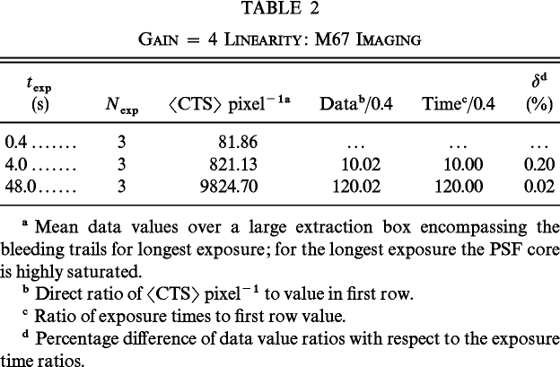
To further probe the linearity at gain = 4 to well beyond saturation a sparse field of bright stars in M67 was imaged using the CLEAR (50CCD) aperture at exposure times providing up to 50 times saturation on the central pixel. These results are summarized in Table 2 for a bright star pair near x,y = 895,395. Tabulated data means are taken over an extraction box including full bleeding trails for the longest exposure case. In this instance, even with an oversaturation equivalent to greater than 4 mag, linearity is maintained to ≪1%.
 |
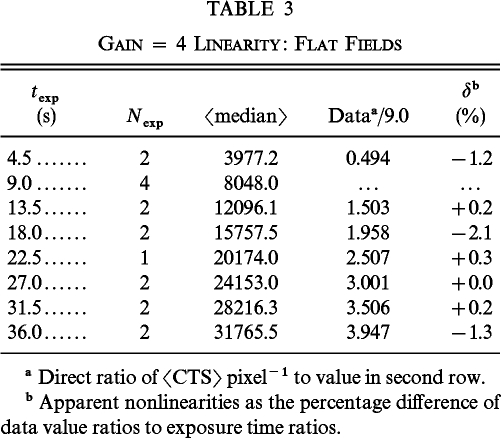
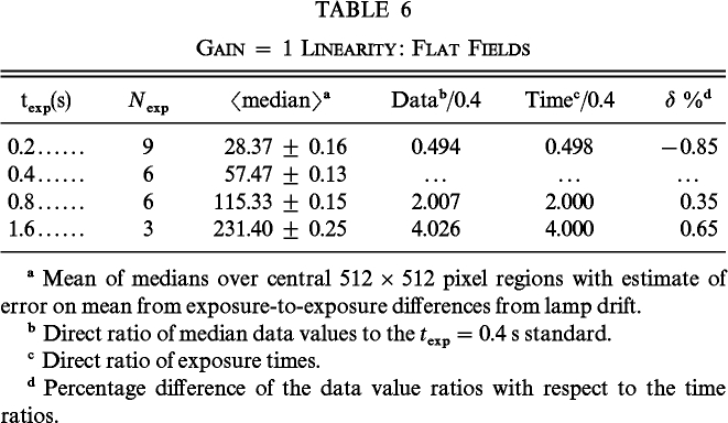
A series of imaging flat fields from 1997 November 11 (using internal calibration lamps) using exposure times of 4.5–36.0 s providing mean exposure levels from ∼12% to 94% of saturation are summarized in Table 3. Exposure times of 9.0 s were interleaved in the series to track possible lamp intensity drifts (corrections based on the 9.0 s exposure values over time were made but never exceeded 0.8%, except for the first exposure in a set which has been ignored). These results follow from two occultation periods of data collection. The tabulated values are the mean at a given exposure time of median values (median used to avoid influence of possible cosmic rays) evaluated over the central 512×512 pixels of the CCD. The confidence level in tracking lamp intensity variations is roughly 1%. The results are consistent with linearity over the range from 12% to 94% of saturation, although the potential lamp variations prevent this from being a very precise test. Preflight data of higher precision gave constraints on linearity over this domain of ≲0.2%.
 |
As with WFPC2 operated at the low gain of 14 e− DN−1 (Gilliland 1994), STIS CCD data at gain = 4 can provide accurate photometry well beyond saturation. (Assuming the bleeding columns do not cross other significant sources, and of course saturation results in loss of spatial information along the columns.) In the STIS gain = 4 case saturation occurs on the CCD, not in the subsequent electronics, thus allowing a trivial summation to include the pixels bled into.
As a final investigation of high S/N and saturated data at gain = 4 we have examined the spectral fidelity of extracted α Cen A and B spectra corresponding to the first six exposure levels in Table 1. We have tracked the following measures of spectral fidelity over the range of exposure times (and thus signal levels): (1) the S/N of the α Cen A and B spectra, defined as the inverse of the standard deviation obtained after ratioing individual spectra to the mean 0.1 s spectrum for each star (after a Fourier domain shift to co‐align), and (2) the depth and width of an isolated, sharp absorption line in α Cen A evaluated via a nonlinear, least‐squares Gaussian fit. These results are shown in Table 4. Unfortunately for these spectra, being only marginally sampled in the dispersion direction, a small amount of drift along the dispersion has significantly compromised simple conclusions. It is clear that for spectra spanning cases of central intensity ∼15% of full well (B at 0.1 s) to ∼3 times saturation that spectral fidelity remains high. Figure 1 compares extracted spectra for α Cen A at 0.1 s (no saturation) and 0.4 s (central 2–3 pixels in cross‐dispersion are saturated). Even with noise introduced by Fourier domain shifting (note the characteristic "ringing" signature of such noise in the bottom panel of Fig. 1) to align the spectra in the dispersion direction, the maximum deviation in the ratio is ±0.7%. Variations in the depth and width of a strong, isolated line (at column 365) are only 0.5% and 0.8%, respectively, with no dominant trend with count level. The drop in S/N with increasing count level probably results to first order from noise generated in shifting (Fourier domain shift used) poorly sampled data, rather than any degradation of intrinsic spectral fidelity. The S/N of A and B spectra (which experience the same shifts) decline in a very similar manner despite the factor of 3 difference in mean count level. The Poisson limits for S/NA and S/NB in the first line of Table 4 are 961 and 555, respectively, with comparable values for the other lines. Entries are not included for the 0.7 and 0.8 s exposures since bleeding occurred beyond the edges of 7 pixel tall extraction boxes.
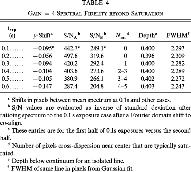 |
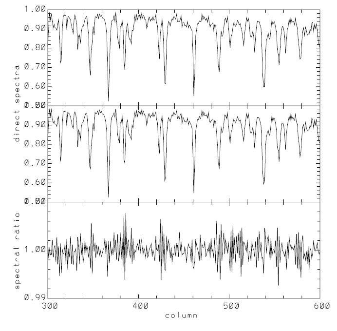
Fig. 1.— The upper panel shows a spectrum of α Cen A using the G430M grating at central wavelength 5471 Å averaged over 32 exposures each of 0.1 s at gain = 4 e− DN−1 yielding a high S/N result without reaching saturation. The middle panel shows the same based on an average of five exposures of 0.4 s, each of which has 2–3 saturated pixels in cross‐dispersion. The bottom panel shows the ratio (after a 0.1 pixel Fourier technique shift of the 0.1 s spectrum) on an expanded scale. Even with strong saturation the response is linear at gain = 4.
Saturation obviously results in loss of spatial information as a result of charge bleeding along columns. For the purposes of point source photometry or spectroscopy, excellent precision and fidelity are, however, maintained to well past saturation.
3. HIGH COUNT LEVEL NONLINEARITY: GAIN 1
As for gain = 4, we took a series of short exposures on α Cen A and B to test for linearity from well below to well above saturation at the high gain of 1 e− DN−1. Saturation in this case is ∼38,000 e− per pixel at the CCD edges increasing to ∼44,000 e− at the CCD center (or a factor of about 3 shallower than gain = 4 saturation in e−). To allow nonsaturation at 0.1 s, a shorter central wavelength (3423 Å) of the G430M grating was adopted here. The behavior at gain = 1 for levels up to saturation is similar to that for gain = 4; again the results at texp = 0.1, 0.2, and 0.4 s are consistent with a small decrement existing on the 0.1 and 0.2 s commanded times. The response beyond saturation shows a steep departure from linearity in stark contrast to the gain = 4 case. The limitation near saturation for gain = 1 was already known from preflight calibration and discussed in the STIS Instrument Handbook (Baum et al. 1998).
Separately extracted spectra for α Cen A and B provide further confirmation of good linearity for gain = 1 up to saturation but poor fidelity beyond. Table 5 presents results at gain = 1 analogous to the gain = 4 case in Table 4. At texp = 1.0 s the α Cen B spectrum reaches ∼90% of saturation for the brightest pixel at longest wavelengths. The full range (see Table 5) of B spectra exposure times therefore map out the range from 10% to 90% of full well depth. The Poisson limit for α Cen A spectral ratios is ∼250 and for B∼110–120 with only mild variation over different exposure times, since the product of texp×Nexp does not vary greatly. The α Cen B spectra maintain excellent fidelity and overall linearity. The only significant departure from linearity (0.5% at 0.1 s exposure time) could be accounted for completely by a small change (<2 σ) to the 0.1 s exposure time correction derived in § 2. The α Cen A spectra at texp = 0.2 s reach to 65% of full well; spectral fidelity drops precipitously beyond saturation.
 |
At gain = 1 e− DN−1 the STIS CCD electronics provide excellent linearity to near saturation, but beyond saturation charge is not conserved (in contrast to the gain = 4 case), and the results are highly nonlinear. We have not attempted to define the character of this nonlinearity further; clearly at high count levels for which the central pixel counts might exceed ∼30,000 e− it would be prudent to use gain = 4 to acquire the data and thus assure inherent linearity.
4. LOW COUNT LEVEL NONLINEARITY AND CTE
We have explored linearity at low count levels in three different ways: (1) with series of low S/N spectra at stepped exposure levels, (2) imaging at low S/N, and (3) with a series of low count level internal flat fields.
Low‐intensity flat‐field exposures were acquired (1997 November 11) only for gain = 1 using four levels of exposure time in factor of 2 steps resulting in exposure levels of 28–231 e− per pixel. The results are tabulated in Table 6 and are consistent with linearity over this domain, to within the roughly 1% accuracy permitted by potential lamp variations. A small deficit at the lower count levels is suggested but not firmly established.
 |
The low count level flat‐field exposures also allow a check for any columns that might show deferred charge—a nonresponsiveness to input until a certain "fat‐zero" is accumulated after which linearity is restored. The full 1024 × 1024 images were analyzed for columns possibly showing deferred charge using standard techniques (see Tyson & Seitzer 1988; Gilliland & Brown 1988). These data support a per‐pixel precision of about 4 e− and less than 1 e− for averages over columns. The results were remarkably clean with no evidence whatsoever of deferred charge behavior on the STIS CCD.
The primary information on low‐intensity nonlinearity follows from series of slitless spectra acquired in two orbits (1997 December 24 and 29) on a sparse M67 field for point source spectroscopy (as opposed to the flat‐field illumination described above). The gain = 1 exposures were taken at four different exposure times of a field covering a range of stellar brightnesses and allow tracking of response over a broad range of CCD signal levels. The full CCD format is used and stars of similar magnitude located at different positions on the format allow testing for positional dependence as would be expected from imperfect CTE.
For the high count level data discussed in earlier sections, careful background subtraction was not needed. At low count levels a correct estimate and subtraction of the background may be important. Ferguson (1996) details issues that can arise in computing sky background for WFPC2 data; the same limitations arise for STIS data, particularly at gain = 4. We have evaluated sky levels as either the mean of points windowed to ±3 σ of the mean, or via taking the centroid of a histogram of sky pixel values over ±3 σ with consistent results.
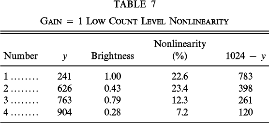
Figure 2 shows the G750M 6768 Å spectral image of the M67 field made from the cosmic‐ray–eliminated sum of four exposures, each of 97.2 s at gain = 1. A direct test of linearity follows from comparing the counts in extracted spectra at this exposure level with the counts extracted from the sum of eight shorter exposures of 3.6 s each (27 times shorter per individual exposure). The star near y = 241 has an average of 1211.13 counts per pixel in dispersion (per long exposure) using an extraction box of 7 pixels cross‐dispersion. The mean is 36.58 counts per dispersion pixel for the short exposure for a ratio of 33.11. The counts in the deeper exposure are 22.6% above the prediction (time ratio of 27) scaled from the shallower exposure. The counts for this star in the shallower individual exposures peak at 17 e− per central pixel, and the extracted sum corresponds to a S/N of 4.4 per dispersion pixel. The substantial nonlinearity observed here represents a significant departure from the behavior observed at similar signal levels in the flat‐field exposures described above.
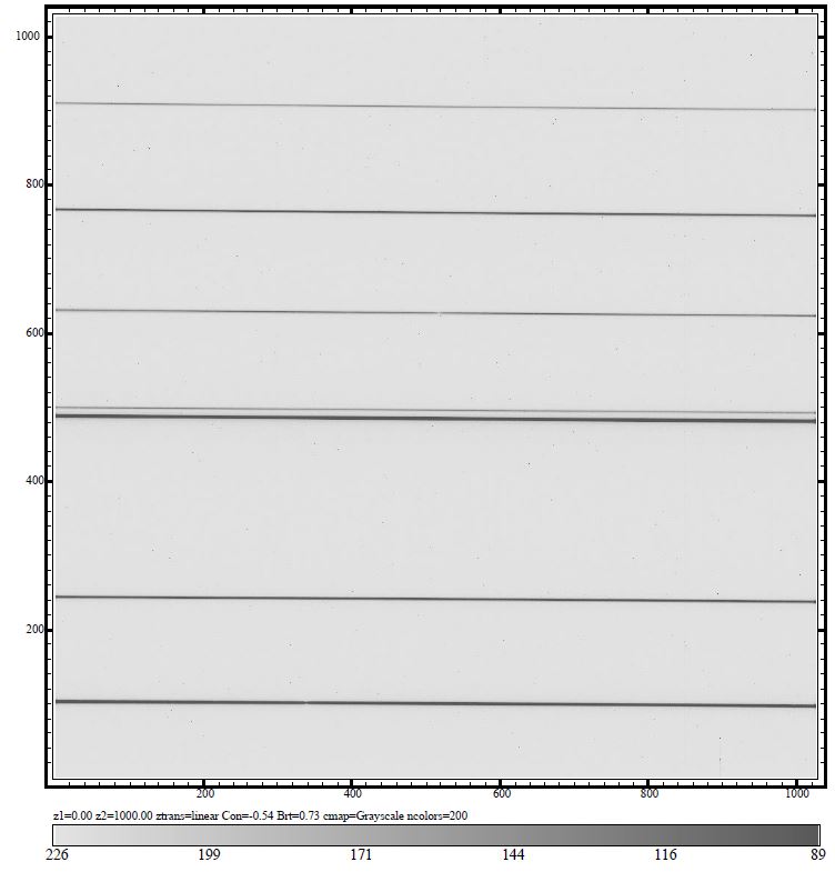
Fig. 2.— STIS CCD slitless spectroscopy image of sparse field of M67 stars used in determining low count level nonlinearity. The coordinates shown are x and y pixels of the CCD data.
Charge loss due to CTE effects is a natural suspect for accounting for the difference observed between the "flat‐field" and "sparse‐field" linearity performance. The STIS CCD readout amplifier is located at the upper right‐hand corner for the Figure 2 display. Imperfect CTE in the parallel clocking direction should thus lead to a successively larger nonlinearity at lower row numbers. The spectrum located at y = 763 is about 25% fainter than that for y = 241; the intensity effect alone would therefore predict a larger nonlinearity for the upper spectrum. The y = 763 long‐ and short‐exposure count means are 962.34 and 31.74, respectively, i.e., a ratio of 30.32—in this case the nonlinearity expressed as the ratio of counts to ratio of exposure times is 12.3%. The nonlinearity is larger for the star at lower row number, despite its being slightly brighter. This is fully consistent with a CTE effect.
Stars at rows 626 and 904 provide an additional check, at the long‐exposure time these spectra average 525.50 and 346.00 counts per dispersion pixel, respectively. Again the star lower down shows a larger nonlinearity of 23.4% compared with only 7.2% for the slightly fainter star at a row near the readout amplifier.
The nonlinearity between 3.6 and 97.2 s exposures for these four stars is summarized in Table 7. These results suffice to demonstrate correlations of the nonlinearity with both y‐position and relative brightness with the expected signs. Mean background levels per exposure ranged from 0.1 e− per pixel for the 3.6 s case to 1.6 e− per pixel at 97.2 s. For these gain = 1 data, uncertainties in estimating sky are not an important limitation.
 |
We have also checked for possible dependence of nonlinearity on the distance from the readout amplifier in the serial clocking direction. We have evaluated the equivalent of Table 7 entries, but using extractions restricted to x = 50–250 and 775–975, respectively. In the case of imperfect serial CTE, we would expect any correlation to show a larger nonlinearity for the lower x interval. The mean difference in nonlinearity (%) between low and high x was less than 2%, which is near a reasonable estimate of a confidence interval given limitations on estimating background, and this showed the larger effect for high x. Hence, any dependence on x must be an order of magnitude smaller than the y dependence. We will assume there is no x‐dependent CTE or nonlinearity for the purposes of further discussion. We realize of course that for spectroscopic applications with the spectral order roughly parallel to the shift register a dependence on x may be masked; it is possible that imaging data would show such a dependence.
Following Stetson's (1998) analysis of WFPC2 corrections to remove the effects of CTE on photometry, we seek a solution to correct STIS CCD spectroscopy for CTE. We allow only for Y‐dependent ramp and the spectral count level expressed as the number of e− per pixel following a standard extraction. The reduced Stetson (1998) equation set (1)–(9) becomes


The corrected count level for spectroscopy is then
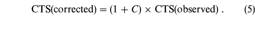
It is essential in applications of these equations to use a consistent definition of CTS: number of e− summed over a 7 pixel cross‐dispersion box per dispersion pixel per individual exposure. (Note that CR‐SPLIT exposures are summed by the pipeline reductions for the CRJ‐EXTENSION data; these would need to be divided by the number of splits and multiplied by the gain value for use here.) Stetson (1998) adopted a "softened" sky in order that the predicted photometric correction approach a finite constant value as the estimated sky brightness approaches zero. Recognizing that our data provide very little leverage to determine the effect of a varying sky background, we further simplified this exploratory analysis by eliminating Stetson's equation (2) and his c2 term. Our derivation may therefore only apply for the limit of negligible sky background (as would often be the case for narrow‐slit spectroscopy of point sources or short‐exposure slitless spectra as in our data). In this solution we have not subtracted the background sky. Since sky is both small and scales with the exposure time, subtracting sky first would only slightly modify the solution. The problem has now been reduced to finding the coefficients c1 and c2 of equation (3) that in a least squares sense account for the nonlinearities of Table 7, but using all seven of the stars in these data.
For each of the seven stars we derive mean extracted spectral intensities at each of the four available exposure times each in three successive ratios (3.6, 10.8, 32.4, and 97.2 s). The faintest star at 3.6 s averages 6.8 e− from a 7 pixel wide extraction while the brightest at 97.2 s reaches 3390 e−. Ratios of the longer exposure time means are taken against the 3.6 s value and further normalized by the ratio of exposure times. This yields 21 values that should average 1.0 for linear response. However, the actual mean and standard deviation of these entries is 1.200 ± 0.212 with a full range of 1.013–1.829.
A least‐squares solution for c1 and c2 in the above equations was found that most nearly gives linearity for all 21 ratios after application of equation (5) to all 28 data values. The resulting mean and standard deviation for ratios formed in the same way as in the previous paragraph after application of this correction is 1.000 ± 0.023 with a full range of 0.949–1.035. Nearly all of the variance in the nonlinearity is accounted for by the combination of position‐ and intensity‐dependent terms. The least‐squares derived coefficients are
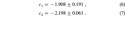
Figure 3 illustrates the correction factor (C of eq. [4]) as a function of the observed number of counts in e− (7 pixel tall extraction box) and at three different y‐positions on the CCD. The overplotted symbols in Figure 3 have a vertical extent of ∼3 σ; in a log‐log plot covering multiple decades, deviations of ±2.3% on average are quite small in a relative sense. For a count level of ∼100 e− at chip center, the correction is ∼6%. This solution may be valid only in the limit of vanishing background level. A formal solution including a background term was derived, but this yielded only a small gain in reduced variance and a positive coefficient implying a divergence of the CTE correction in the limit of sky approaching infinity—opposite of the expected physical behavior. A data set with a larger range of intrinsic background would be required to further delineate whether a large background can suppress CTE losses as is the case for WFPC2 (Stetson 1998).
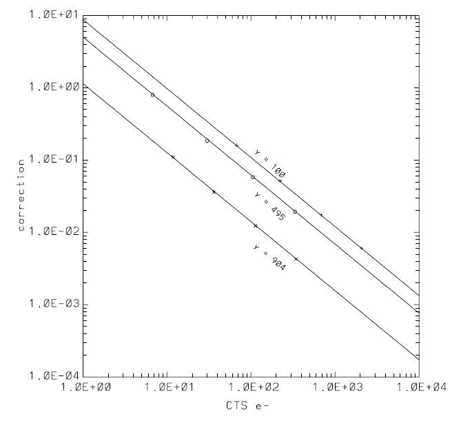
Fig. 3.— Correction factors (C of eq. [4]) as a function of the extracted spectrum count level in e− per dispersion pixel for three different y positions on the CCD. Overplotted symbols show the residual relative deviation from linearity following the correction of observed values. The largest fractional deviation of 0.954 for the second count level of the star at y = 495 is a 2.5 σ deviation.
Equations (1)–(5) may be applied to extracted spectra for which the CTS are in e− units. In principle, this should not only accomplish a linearization for incorrectly lower mean count levels as a result of the parallel clocking CTE, but should also result in maintenance of better spectral fidelity (line cores will experience a differential CTE effect in comparison to nearby continuum). This can be tested by applying equations (1)–(5) to linearize high and low exposure level spectra and checking to see that spectral features better match after this correction. In a formal sense this works well for the lowermost star in Figure 2; a direct ratio of longest and shortest exposure time spectra yields an rms scatter of 0.25, which drops to 0.15 after correcting. However, none of these spectra contain strong lines and the improvement merely follows from suppressing the effect of extraction values that happened to scatter too low in such low S/N, short‐exposure spectra. We believe it is safe to assume this correction can be applied pixel by pixel to extracted spectra, but we do not have sufficient data in hand to definitively test this assertion.
A CTE effect of the type we have modeled above should be independent of gain which is set in electronics after the CCD. Our gain = 4 data in this experiment cover a smaller range of exposure times (8.6 vs. 27.0) than the gain = 1 data. Coupled with a greater difficulty in adequately determining sky, the gain = 4 data are not useful for an independent solution. However, application of equations (1)–(5) for the best available test case resulted in the linearity ratio dropping from 1.24 to 1.05. This serves as at least weak confirmation that with the count level expressed in e− equations (1)–(5) may be applied independent of selected gain.
Since spectroscopic and imaging data present a different profile of e− relative to CCD pixels and parallel clocking, we do not expect that identical CTE correction coefficients should apply in the two cases. In particular, given the two‐dimensional aspect of an imaging point‐spread function (PSF) in comparison to one dimension for spectral extractions, a greater contribution to a given sum arises from lower count level pixels in the case of imaging. Thus a CTE effect may be manifested at larger amplitude for point sources. We have used equations (1)–(5) in conjunction with exposures at 0.1, 0.3, 0.4, 0.9, and 4.0 s on a sparse field of five stars in M67 to estimate a CTE correction for imaging applications. As with our spectral data, the background sky level is too low in all the images to support tests for possible suppression of CTE effects at high background. The faintest of the M67 stars has 224 e− in the 37 pixel extraction aperture used (S/N∼7.5) with a 0.1 s exposure. The brightest star has 440,000 e− in 4.0 s. A table of data ratios normalized to the exposure time ratios has a mean and rms of 1.026 ± 0.078. After a solution for c1 and c2 and application of equations (1)–(5) the ratios have a mean and rms of 0.989 ± 0.026 and the maximum deviation drops from 1.24 to 1.06. The imaging coefficients for equation (3) are

This solution has larger errors than the spectroscopic solution due to a poorer sampling of relevant exposure levels and y‐distribution of stars on the CCD in the available data. The derived position dependence is similar to, and well within the mutual errors of, the spectroscopic solution. The intensity dependence is stronger for imaging, although the larger error places the significance of this statement at only the 1 σ level. These results are qualitatively consistent with the CTE interpretation. The fainter stars in the M67 exposures happen to lie near the CCD diagonal; therefore it was not possible to test independently for a possible x‐dependence on the CTE.
Having established with this exploratory calibration program that low count level data are strongly biased by a CTE effect, a more robust calibration will be defined to (1) search for time evolution in the basic effect, (2) determine if significant background levels suppress CTE losses, (3) obtain a more accurate CTE correction for imaging data in particular, and (4) determine whether x‐dependence on the CTE induced nonlinearity exists.
The low signal level CTE performance derived here represents a significant departure from the performance observed during preflight calibration. Analogous "sparse field" tests in the ground calibration period indicated that departures from linearity for point source spectra were less than 1% down to signal levels of 100–200 e− per column (in contrast to the ∼6% effect at 100 e− level derived from the in‐flight fit). As there are no other indications of changes in the performance of the CCD readout electronics since launch, we are inclined to attribute the apparent CTE degradation to radiation damage effects in the orbital environment.
While CTE degradation is expected due to displacement damage in the CCD silicon (primarily from South Atlantic Anomaly protons), the change implied here is surprisingly large for only 0.9 years in orbit and shows a surprisingly steep dependence of the correction factor C on signal level. However, if the apparent change since launch is correct and radiation damage is indeed the cause, the CTE effects should continue to grow in proportion to the accumulated radiation dose. Hence, the correction parameters derived here would be effective for only a narrow time window around the date of these observations. Clearly a regular monitoring program, involving methodologies similar to those employed here, will be required (a) to determine definitively whether there is an ongoing trend of CTE degradation and (b) to permit derivation of revised correction parameters as time progresses to assist in the accurate calibration of scientific data.
It is worth noting that some operational remedies are potentially available for ameliorating the effects of CTE degradation. The STIS CCD has separate serial registers at each end of the chip; each has at least one low noise amplifier. The flight software is capable of supporting a "split‐parallel" readout mode that would decrease the number of row transfers and thus CTE losses by a factor of 2. Alternatively, for observations not requiring the full 50 '' CCD field, the telescope could be pointed to position the region of interest closer to the serial register, again decreasing the number of parallel transfers and the corresponding CTE losses.
5. HIGH S/N TIME SERIES TEST AND SHUTTER STABILITY
Reaching the extreme S/N domain that would be needed to detect the analog of solar p‐mode oscillations (see, e.g., Brown & Gilliland 1994) has not been a goal for any HST instrument during definition and development. With amplitudes of only a few parts per million (ppm, or equivalently to within a factor of 1.086 conversion, micromagnitudes [μmag]) detection of strict solar‐analog oscillations on other stars requires a time series with resulting noise of 1 μmag per independent frequency. This in turn, as an example, would require accumulating 10,000 measures if each reaches "only" a S/N of 10,000. Such extreme S/N per exposure requires counting 108 e− per readout according to Poisson statistics. (Observations from the ground are limited by atmospheric scintillation to values of this order even on 4 m telescopes at the best sites using 1 minute integrations, the gain with aperture size is slow, and the resulting noise is often non‐Gaussian; e.g., see Gilliland et al. 1993.) By observing above the atmosphere, HST is not limited by atmospheric scintillation. However, the desire to image into very few pixels in order to maximize sensitivity for faint objects restricts WFPC2 or STIS imaging to ∼2.5 × 10⁵ e− per readout for a S/N of ∼500—not remotely close to the levels needed. The STIS CCD can of course be operated in a mode (normal spectroscopy) that "smears" the PSF over a full row of pixels allowing 3 orders of magnitude more counts per readout. Using the STIS CCD in spectroscopic mode allows collection of ≳108 e− before saturation and in principle would support S/N≳10,000 per readout. (With a requirement of 10,000 exposures, given a minimum current readout time overhead of 20 s would still require a significant 35 orbit investment to reach μmag sensitivity. However, stars with moderately larger expected mode amplitudes could be studied with quadratically less time to reach marginal detection thresholds.)
In order for the STIS CCD to provide high S/N observations capable of approaching the μmag level on single stars at least two constraints must be satisfied:
- 1.The CCD, associated electronics, and the HST pointing system must allow the Poisson limit to S/N to be nearly maintained to count levels of ∼108 e− per readout.
- 2.The camera shutter timing (length of time open) must be repeatable to less than 10−4 of the exposure time to be used.
A direct determination of the STIS CCD shutter‐timing repeatability was not available from ground testing. Ground test measurements confirmed that the shutter exposure times were accurate to better than the 5 ms level specified but did not quantify the exposure‐to‐exposure variations to the precision necessary to assess the viability of the high S/N time series analyses considered here. In order to measure the shutter stability, we obtained a series of 32 spectroscopic exposures on α Cen A and B simultaneously using the minimum exposure time of 0.1 s. A grating setting was selected to yield ∼108 e− on α Cen A and a factor of 3 less than this on B. Intrinsic variability of these stars over the time span of ∼10 minutes for this test should be at the level of ≲10−5 from either oscillations or stellar activity; therefore for the purposes of this test we may assume the sources are both constant. The expected Poisson limit S/N on B of ∼4000 per exposure provides the limiting goal of these analyses. Spectra for both A and B were extracted using 7 pixel boxes centered on the flat‐fielded spectra. A correction for sky is not relevant at these extreme count levels. Cosmic rays were searched for on a pixel‐by‐pixel basis over the stack of 32 exposures as multi‐sigma positive deviations; it was easily verified that cosmic rays were not significant for the error budget. Shutter timing fluctuations of ≳0.1/4000 × 2 = 5 × 10⁻⁵ s should be made apparent as correlated changes in the A and B time series.
The total signal per exposure (sum of counts) divided by the rms deviation in the time series was ∼460 for both A and B, or an order of magnitude below the Poisson limit. (Note that atmospheric scintillation for 0.1 s exposures from the ground would limit this S/N to ∼200 for a 2.4 m telescope; see Young 1967.) The A and B time series had a linear correlation of greater than 0.98 showing that most of the variance in either was induced by some common external factor—most likely minor fluctuations in how long the shutter remained open. Other sources of correlated noise are possible, e.g., from x, y pointing differences between exposures, and jitter or focus changes that lead to altered fractions of energy enclosed in the extraction boxes. Once S/N of several thousand is sought, close attention must be paid to many subtle factors. We will therefore present results for a systematic time series analysis including allowance for these several sources of correlated noise.
These G430M spectra centered at 5471 Å on α Cen A and B display a large number of strong, sharp lines. Exposure‐to‐exposure relative offsets along the x, or dispersion direction, were evaluated using a simple cross‐correlation technique (see, e.g., Brown & Gilliland 1990). The observations were conducted while α Cen was in HST's Continuous Viewing Zone; therefore the pointing is near the orbit pole and orbital Doppler motions are small. In the y, or cross‐dispersion direction, offsets were determined by fitting a Gaussian in cross‐dispersion at each pixel along both of the A and B spectral orders separately and forming a grand average of the results. The resulting rms values in x and y were 0.063 and 0.081 pixels, respectively, or 0 0032 and 00041 equivalent, i.e., fairly typical jitter values for HST guiding (the specification is less than 0007 which is usually improved upon by 50%–100%). The maximum deviations were at about 3 σ, consistent with a generally Gaussian noise distribution. The Gaussian fits in cross‐dispersion also provided a measure of spectral width (FWHM) which varied with an rms of 0.015 pixel; this is equivalent to 00008 and could arise from differing levels of cross‐dispersion motion within exposures.
We find that significant noise in the time series on both A and B correlates with the x,y offset and spectral order width variations. The S/N on either A or B then follows only after evaluating a simultaneous linear least‐squares regression of the A or B time series against B or A (to remove shutter variation imposed noise) and the x, y and width parameter variations. Although the Poisson‐limited S/N on A is much higher than for B, with shutter variability introducing the largest variance for these short 0.1 s exposures, the intrinsic Poisson noise on B also limits the ultimate S/N that can be reached for A.
The summed counts on individual A and B extractions (summed over columns 68–524, the first chosen to place the start clear of strong lines, the second to place the end before the order slope leads to B crowding the subarray limit) are 5.74 × 10⁷ and 1.92 × 10⁷, respectively, for inherent Poisson‐based S/N limits of 7576 and 4382. With the need to regress A and B against each other, the limiting S/N drops to 3792 for both [from (1/75762 +1/43822)1/2]. The realized time series S/N is 3250 following regressions described above. We have checked that no trends exist in the time series residuals, and averaging residuals in blocks of four results in a full factor of 2 drop in rms variation—the input time series, external parameter decorrelation vectors, and resulting residuals can apparently be well represented as simple Gaussian (white) noise. We have performed extensive Monte Carlo simulations generating A and B time series with independent Poisson noise, imposing identical Gaussian noise fluctuations as would follow from shutter timing and Gaussian noise x, y, and width decorrelation vectors. This Monte Carlo simulation returns the expected S/N limit of 3792 and shows that a significant rms variation of 482 applies when only 32 points and four variable parameters exist to regress against. Our result of 3250 for the real data therefore deviates on the low side by 1.1 σ. We would expect results to be low if there is (1) any measurement noise on the regression vectors or (2) other sources of noise exist that have not been accounted for. (The ability to cleanly define the regression vectors usually improves with the number of independent measures. In this context 32 is small; however, compared to broad experience with ground‐based high S/N efforts, these data are clean and easy to work with.) Fractional noise in the direct A time series is ≲10−4 from each of x and y image motion, ∼1.3 × 10⁻⁴ from intrinsic Poisson, ∼2.3 × 10⁻⁴ from spectral order width variation and a dominating 2.0 × 10⁻³ term from correlated A and B noise which we attribute to shutter timing fluctuations. Stability at 0.002 with 0.1 s exposures implies rms variations in the exposure times at a very modest 0.0002 s.
If the exposure timing error is a simple additive term then its relative importance will decrease linearly with exposure time. For example at texp = 10 s, still only 50% of the minimum overhead time to cycle the STIS CCD with small subarrays, the relative contribution would be at 2 × 10⁻⁵ implying a limiting signal‐to‐noise on single targets of 50,000. We have a partial test of this through shorter time series on α Cen A and B (see Table 1) at longer exposure times. This calibration proposal was written without the benefit of knowing the shutter is managed differently at 0.1 s (see § 2); with the benefit of hindsight a primary time series using ∼1 s exposures would have provided more direct results. Furthermore, simple interpretation is limited by the following: (1) with only seven or five points in a time series, decorrelation against four independent variables produces wide variations in pure noise trials, and (2) α Cen A begins to saturate already at texp = 0.3 s. A formal analysis of resulting time series S/N for the longer exposure cases is consistent with a strong drop in relative importance of the shutter term. However, without imposing additional assumptions this result is without statistical significance. (An exception was that the 0.2 s time series showed a larger contribution from shutter timing variations. This is reasonable given the § 2 discussion on shutter management.) If we assume that the fractional noise contribution from x, y and width variations remains constant, then the resulting S/N for the longer time series is consistent with a falloff of the timing fluctuation proportional to t-3/4exp. If this weaker than linear dependence (not considered a robust determination) holds, then 10 s exposures would still provide S/N∼15,000 per exposure.
6. SUMMARY AND DISCUSSION
We have explored a number of areas related to limiting performance of the STIS CCD on HST relevant to both low and high S/N regimes.
With a gain = 4 e− DN−1, the CCD and associated electronics provide excellent linearity at high count levels, even in the sense that charge is linearly conserved to well beyond saturation of individual pixels (with summation over pixels bled into). This linear behavior at high count levels extends to excellent retention of spectral information even when the central pixels are oversaturated. With a gain = 1 e− DN−1, significant deviations from linearity arise as the input signal reaches and exceeds nominal saturation. A clear preference for gain = 4 exists for work at high S/N, and the penalty imposed by a slightly higher readout noise at the lower gain is negligible at high count levels.
At low count levels a strong nonlinearity arises. Spectra at low count levels have fewer counts than would be expected from scaling a better exposed case down by the exposure time ratio. Strong correlations with intensity and y‐position on the CCD are clear from inspection of a few extractions as would be expected from imperfect CTE in the parallel clocking direction. A simple two‐term model accounts for nearly all the nonlinearity measured in the gain = 1 calibrations. The model also seems to work well for gain = 4 data as would be expected for a CTE effect. Further observations will be required to better characterize this effect, to determine any evolution with time, and to establish appropriate corrections for application to science data.
The STIS CCD operated in a spectral mode in order to disperse the light over many pixels can support ultrahigh S/N, rapid time series photometry. We demonstrated that the STIS shutter control produces timing fluctuations at the level of ∼0.0002 s and that the relative importance of this falls off steeply (perhaps linearly) with increasing exposure time. In a primary trial observing α Cen A and B simultaneously time series with S/N = 3250 per exposure was directly demonstrated. This result was close to the Poisson limit for the experiment as designed. Although not directly demonstrated here, we see nothing to suggest that with longer exposure times (5–10 s in this case) and count levels ≳108 e− per exposure that the STIS CCD and HST would not support S/N to 10,000. Indeed, the remarkable stability seen for gain = 4 at and beyond saturation suggests the possibility of exploiting even higher count levels to perhaps allow time series S/N well in excess of 10,000 per exposure.
Footnotes
- 1
Based on observations with the NASA/ESA Hubble Space Telescope, obtained at the Space Telescope Science Institute, which is operated by AURA, Inc., under NASA contract NAS5‐26555.