
Abstract
Measuring changes in the characteristics of corticospinal output has become a critical part of assessing the impact of motor experience on cortical organization in both the intact and injured human brain. In this protocol we describe a method for systematically assessing training-induced changes in corticospinal output that integrates volumetric anatomical MRI with transcranial magnetic stimulation (TMS). A TMS coil is sited to a target grid superimposed onto a 3D MRI of cortex using a stereotaxic neuronavigation system. Subjects are then required to exercise the first dorsal interosseus (FDI) muscle on two different tasks for a total of 30 min. The protocol allows for reliably and repeatedly detecting changes in corticospinal output to FDI muscle in response to brief periods of motor training.
Introduction
The organization of adult corticospinal output is highly dynamic. Animal experiments using intracortical microstimulation and human experiments using transcranial magnetic stimulation (TMS) have demonstrated changes in motor map size and excitability in response to a variety of manipulations, including central1,2,3,4,5 and peripheral6 stimulation, pharmacological interventions7,8 as well as differential sensory9,10,11 and motor12,13,14,15 behavioral experiences. Such corticospinal plasticity is thought to represent a neural mechanism supporting motor learning in the intact brain and motor relearning/reorganization in the damaged brain16. Thus, reliable and repeatable measures of experimentally inducible corticospinal plasticity may provide insight into the capacity for both normal motor learning and motor recovery after brain injury.
Rapid, short-term increases in corticospinal excitability have been reported to occur in response to brief periods of motor training17,18. Developing a reliable method for measuring such changes in corticospinal output could serve as a clinically useful method for measuring the capacity for motor cortex plasticity that may vary as a function of age, brain injury or neurological disease. One of the difficulties with this approach has been demonstrating changes in the topography of excitability with respect to specific cortical areas. Animal studies where the brain is exposed and stimulation points are targeted using a grid superimposed onto the cortical surface allow for detailed examinations of corticospinal output using fine microelectrode manipulation19,20. Surface vasculature and stereotaxic coordinates can then be used to detect subtle changes in corticospinal output that occur in response to a variety of experimental manipulations16.
This technique has been more difficult to achieve in human subjects using TMS, where superimposing a grid onto the cortical surface in order to repeatedly and reliably position the TMS paddle across cortex is not easily achieved. The advent of new frameless stereotaxic methods that integrate MRI with TMS now allows for more precise localization and anatomical co-registration of muscle representations21,22,23. This approach has also improved the consistency of TMS measures22, reducing the variability associated with different experimenters. Here we describe a method for assessing corticospinal plasticity that takes advantage of this new technology and employs a grid method used in rodent and non-human primate microstimulation experiments. Furthermore, we show that this technique is sensitive enough to detect changes in the size and excitability of FDI representation unilaterally, after as little as 30 min of exercise. The technique may provide a simple assay for measuring the capacity of motor cortex for functional reorganization in a variety of clinical populations and has the capacity to improve translation of insights gained in animal studies to human investigations24,25,26. While the methods described herein pertain to short-term training in the motor system, they can likely be readily adapted to other systems in which TMS has utility, such as memory, language and attention, and further can be adapted to other contexts such as long-term behavioral effects and virtual lesions.
Overview of procedure
The experiment involves first acquiring the anatomical MR, creating the cortical surface grid, registering the subject's head to the MRI in Brainsight, acquiring pre-training TMS measures, motor training and acquiring post-training TMS measures (Fig. 1).

An anatomical MRI is first acquired that is then imported into the Brainsight software, where a 3D image of the subject's brain is constructed. Using this software and Canvas imaging software, a grid is superimposed onto the cortical surface. This is done before mapping the subject. During mapping, the 3D image is first registered to the subject's head using facial landmarks. The sight of lowest motor threshold (SOLMT) is found using transcranial magnetic stimulation followed by a recruitment curve used to examine stimulation current motor evoked potential (MEP) amplitude relationships. The total area for first dorsal interosseus representation is then determined. The subject then performs 30 min of motor training, after which the same recruitment curve and representational areas are derived. Analysis of MEP amplitudes and map area is conducted offline.
Materials
Reagents
-
Human subjects (see REAGENT SETUP)
Equipment
-
MRI scanner (at least 1.5 T) (e.g., Phillips)
-
Digital microcalipers, 0.01 mm resolution (e.g., Avenger Measuring Tools)
-
Stereotaxic neuronavigation system (Brainsight; Rogue Research)
-
Head support/chin rest system (Brainsight; Rogue Research)
-
Polaris tracking system (Rogue Research)
-
TMS 70-mm figure-of-eight coil and stimulation system (e.g., a Magstim 2002 from Magstim)
Critical
Although for most materials, alternative brands could likely be substituted with equal results, one aspect where inter-lab differences might emerge is the choice of TMS system. Differences in coil size, shape and pulse can influence TMS measures27,28. For example, the current methods were defined using a Magstim 2002, which employs a biphasic pulse, but use of a monophasic pulse could modify results. Changes in TMS system components in the current protocol might therefore require further study.
-
Foam ear plugs
-
Surface belly-tendon electromyogram (EMG) electrodes, electrode cream and adhesive
-
EMG amplifiers (Grass-Telefactor)
-
Analog to digital converter (AD Instruments)
-
48-inch wraparound saline-soaked felt/Velcro ground
-
Physiological saline
-
EMG recording software (e.g., Scope EMG software, AD Instruments)
-
Graphic imaging software to generate static image (e.g., Canvas X, Deneba)
-
Two computer monitors
-
Computer keyboard with extended cord, to be accessible to subject
-
Jamar Pinch Grip strength force transducer (Sammons Preton Ryan)
-
Stopwatch
-
Small table
-
EMG leads (Integra Neuro Supplies)
Reagent setup
-
Human subjects Human subjects who are eligible for both MRI and TMS, each with its inherent risks, can be recruited. Handedness should generally be assessed and documented, preferably using the Edinburgh Handedness Inventory29. Incorporation of prior recommendations maximizes safety. Thus we recommend you screen subjects appropriately (see Box 1 and refs. 30,31), set stimulation parameters and follow the study conduct recommended in refs. 32–35. Recognizing and managing potential complications of a TMS study has been discussed in these prior reviews. Familiarity with these issues before initiation of TMS also maximizes subject safety.
Caution
This protocol must be approved by the appropriate Human Subjects Committee or Institutional Review Board and be in accordance with the Declaration of Helsinki. It must also conform to appropriate national regulations.
Critical
Informed consent must be obtained from all subjects.
Equipment setup
-
For position of subject and experimenters see Box 2.
Procedure
Subjects
-
1
Obtain informed consent from subjects for TMS and MRI procedures and document handedness. Complete screening and approve this (see REAGENT SETUP and Box 1). Contra-indications to TMS and MRI often pertain to implanted materials such as a cardiac pacemaker or brain aneurysm clip, history related to seizure, history of craniotomy or an unstable medical condition30,31. Box 1 lists specific contra-indications.
MRI acquisition
-
2
Obtain a single, high resolution, T1-weighted volumetric anatomical MRI scan for each subject. Typical parameters are 1-mm3 isotropic voxels, in-plane resolution at least 256 × 256, repetition time = 13 ms, echo time = 4.5 ms and flip angle = 20°, with 1-mm-thick slices and no interslice gap. The imaging field of view must extend from the skull vertex to the bottom of the ears, from the tip of the nose to the back of the skull, and laterally such that the entire pinna is visible on both sides. This is to allow for proper registration of this MRI to the subject's head later, just before TMS, using the neuronavigation system software (http://www.rogue-research.com/TMS.html).
Image processing: creating then sizing the composite MRI of the cortical surface
-
3
Import MRIs into the computer running the neuronavigation system program. We have been able to complete a scan and transport then fully process images rapidly, such that a TMS session can be scheduled 30 min after completion of MRI acquisition. Open the images in the neuronavigation system and create a 3D composite image. As per instructions in the neuronavigation system program, trace the outline of 10–12 sections in the coronal plane, typically from frontal to occipital pole. The first section to be drawn is the midsagittal; place subsequent sections equidistant from this section in alternating anterior and posterior directions. This approach minimizes distortion. View the final image in the 3D mode. Setting the neuronavigation system surface peeler function to peel down 6 mm provides a clear view of the cortical surface, including the entire precentral gyrus from vertex to approximately the Sylvian fissure and is recommended.
-
4
Measure the distance from the nasion to the tip of the subject's nose at midline using the digital microcalipers. View the 3D brain image with the full skull and facial profile visible. Measure the on-screen nose length, again from the nasion to the tip of the nose, using the microcalipers. Enlarge or shrink the image in the neuronavigation program using the zoom function, until the on screen nose length equals the actual distance measured on the subject. The on-screen brain image should now be actual size. View the image without the skull and face tissues.
Critical Step
This step is critical to maintain the desired size of the grid that will be superimposed onto the brain.
Pause point
Steps 2–3 should be done before the TMS mapping session and the images should be saved for each subject for all further sessions.
Superimposing the stimulation grid onto the MRI
-
5
Identify sulcal anatomy on each subject's brain so that the stimulation grid can be superimposed in a standardized manner. Identify the central sulcus first, using all three cardinal views in the neuronavigation program (Fig. 2). This sulcus is found by first following the superior frontal sulcus posteriorly to the first sulcus it intersects, which is the precentral sulcus. This intersection is the most invariant human brain sulcal relationship36. The central sulcus is immediately posterior to the precentral sulcus. Follow the central sulcus dorsally, and place a red marker on the cortical surface where the central sulcus reaches the midline (Fig. 3a), using the marker placement feature of the neuronavigation program. If the central sulcus stops just short of the midline, a projection of this sulcus to the midline should be used.
Figure 2: Anatomical MRI scan showing key landmarks for identifying the central sulcus. 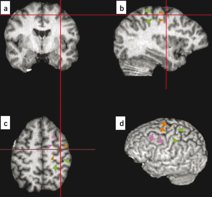
Figure shows the position of the primary motor cortex in a (a) coronal, (b) sagittal, (c) axial and (d) whole-brain image. First, in an axial brain section toward the dorsal brain (c), the slice showing the intersection of the superior frontal sulcus (pink arrowheads) and the precentral sulcus (orange arrowheads) is identified. In all three views, the red hashmarks intersect at the site where these two sulci intersect. The sulcus behind the precentral sulcus is the central sulcus (green arrowheads). By viewing all three cardinal views simultaneously, one can identify the central and precentral sulci in the sagittal view (b). By moving down the central sulcus along its dorsal/ventral course, one can then identify this structure, and stimulate with respect to its location, within any axial slice.
Figure 3: Composite MRI showing the positioning and targeting of the grid markers and a sample motor map for the first dorsal interosseus muscle. 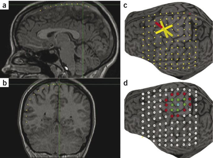
(a) Sagittal MRI showing the position of grid markers (yellow dots) along the midline. The point where the central sulcus was determined to meet the midline is shown as a red dot. (b) Coronal MRI showing the position of markers in one coronal plane of the grid. (c) Three-dimensional MRI showing the completed 10 × 10–point grid across the cortical surface. The transcranial magnetic stimulation (TMS) coil (yellow cylinder extending toward the cortical surface from the red cylinder) can be sited to each grid point using Brainsight software. (d) A sample map of right first dorsal interosseus muscle generated in a separate graphics program (Canvas X). The sites of lowest resting motor threshold (blue dot), positive (green dots) and negative (red dots) responses to TMS are shown; white dots indicate sites that were not evaluated.
-
6
Place markers over the brain on successive coronal images. First, display the midsagittal section in one of the neuronavigation program window panes. In a separate pane, display the coronal plane where the central sulcus reaches the midline. In the hemisphere to be stimulated by TMS, place sequential digital markers along the cortical surface of this coronal section. Space these markers exactly 1 cm apart on the computer screen, verifying the distance using the microcalipers, and follow the contour of the cortical surface (Fig. 3a). Place a total of ten markers (a red one where central sulcus intersects midline, eight yellow ones anterior to this, and one yellow one posterior to the red marker). Note that the number and distribution of markers can be varied depending upon details of study design and TMS target.
-
7
Identify the ten coronal sections containing each of the individual markers. In each of these sections, place markers down the lateral aspect of the cortex. Place ten markers exactly 1 cm apart, again verify this using the microcalipers, beginning at midline and following the cortical contour 6 mm below the surface (Fig. 3b). The use of a 1-cm spacing is intended to minimize errors found with large grid point spacing distances37. Use of this approach ensures that the markers will be visible on the 3D image. Repeat for all ten coronal sections, which will result in a 10 × 10–cm2 grid in the 3D image that covers the cortical surface of precentral gyrus, postcentral gyrus and premotor areas (Fig. 3c). The markers that comprise this grid are to be used to site the TMS coil during mapping.


Creating the static image of the cortical surface and stimulation grid
-
8
Rotate the view of the 3D brain image with the markers slightly in the neuronavigation program along the long axis of the brain such that the entire dorsal aspect of the hemisphere to be stimulated, along with all of its cortical surface markers, is clearly visible (Fig. 3c). Capture this image using a screen capture, and save as a tagged image file format file. Open this image in the graphics program and size to fit the page.
-
9
Use the grid created in Steps 6–8 to create a framework in the graphics program for recording TMS responses. Center a white numbered circle over each marker. The white circles now correspond to the targets that are successively stimulated during TMS, and the image they comprise will now be used to record the location of positive and negative responses elicited during TMS mapping. Thus during mapping, each white circle is changed to a different color to denote stimulation results: a negative TMS response is indicated by red; a positive TMS, by green; and the positive site with the lowest resting motor threshold ('hot spot', Fig. 3d), by blue.
-
10
View the static image created with the white circles next to the neuronavigation program 3D brain image with markers created in Step 9. Viewing both simultaneously, on two adjacent computer monitors, allows for easy integration of grid-based stimulation targeting and recording of responses. Note that MEP waveforms, visualized using a program such as Scope (AD Instruments), can be viewed on either monitor, though we have found it useful to view the MEPs on a monitor separate from the neuronavigation system.
Pause point
Steps 5–10 can be completed before the subject is brought in for testing, or, depending on study design, can be done in less than 30–40 min. Both the neuronavigation system brain image with the markers and the static image with the static stimulation grid can be saved and used for the same subject across multiple testing sessions.
Electrode placement and MEP recording
-
11
Place electrodes over the target muscle(s) corresponding to the movement of interest. The abductor pollicis brevis (APB)17 and FDI4 muscles are two commonly chosen muscles given the ease with which MEPs can be isolated and recorded from them, though many other muscles have been mapped in the literature. For FDI muscle recordings, place one surface electrode on the muscle's proximal tendon, on its dorsal and lateral aspect (i.e., slightly to the thumb side), thus on the dorsal aspect of the index finger between the mid-metacarpal bone and the metacarpophalangeal joint. Place the second electrode over the mid-belly of the FDI muscle, identified by having the subject forcefully adduct the index finger. The electrode placement described here is for one muscle, the FDI. Representation of any other muscle could likely also be evaluated using the current methods. Further details on electrode lead placement for various muscles can be found in any standard electromyography text38.
-
12
Place a ground electrode on the skin overlying a bony region of the wrist. Place a second ground at the base of the neck. Soak the felt Velcro wraparound in saline and, when still rather moist, place very snugly around the upper portion of the biceps ipsilateral to the FDI under study.
-
13
Record motor evoked potentials using amplifier gain of 10,000 plus bandpass filters set from 30 to 1,000 Hz. Suggested settings for the oscilloscope-emulating software include recording at least 1,000 samples s−1; a time window for most studies of 50–200 ms including 30 ms of pre-trigger data, which approximates 10–40 ms inch−1; and a y-axis that extends from −1 to +1 or −2 V +2 V, depending on the muscle and device stimulation settings. This approximates 200–400 μV/8 inch, or 25–50 μV inch−1.
Pre-training TMS
-
14
First, localize the site of lowest motor threshold (SOLMT). To do this the TMS coil (70-mm figure-of-eight Magstim 200 or 2002), with its attached trackers, is registered to the neuronavigation system before the study. Get the subject to don a tracker, too, via the headband or glasses supplied with the neuronavigation system.
Critical Step
To maintain consistent registration throughout the study, it is very important that the subject's headband/glasses not be moved to any extent once the study has started. We prefer the glasses, and have added an adjustable sports strap in the back of the glasses on each side; the strap wraps behind the head where an adjustable element allows a snug and comfortable fit. However, studies of the posterior or lateral cerebrum might need to avoid glasses to approach the stimulation site.
-
15
Register the subject's MRI scan to his/her head using the tip of the nose, nasion, left and right ear tragus as fiducial markers, as described in the neuronavigation system software. Once the 3D MRI is registered to the coil and to the subject's head, integrate the static image of stimulation targets on the cortical surface with standard TMS approaches to measure corticospinal output in a manner that is standardized between subjects and within subject over time39,40. Each stimulation target should be sited in the neuronavigation system using the sulci and gyri and the static image containing the stimulation targets (Fig. 2c).
-
16
Optimize the initial conditions for stimulation. Stimulation should be started at the site closest to the hand knob of the precentral gyrus where FDI representation is known to be located41,42 (e.g., site 65 in Figure 3d). Stimulation intensity can be initially set at 50–65% of the TMS unit's output, which is higher than the normal resting motor threshold of 40% TMS-stimulator-unit output for FDI14,43 and 49% TMS-stimulator-unit output for APB44. If fewer than 6/10 MEPs ≥ 50 μV are observed, the output is increased by 2%. This is repeated until an MEP ≥ 50 μV is observed in at least 6/10 pulses. The current is reduced by 1% increments until fewer than 6/10 MEPs ≥ 50 μV are observed. The current is then turned up in 1% increments; when 6/10 MEPs ≥ 50 μV are again observed, the level of unit output is the resting motor threshold for that brain site. In order to minimize any effects that the TMS probe has on brain function itself, at least 7 seconds is allowed to lapse between each stimulation pulse and the minimum possible number of stimulations should be given across the study. In this regard, the TMS sessions should be kept as short as possible and conducted with the highest of time efficiency to reduce variance from a number of nuisance sources. The position of the TMS coil requires careful attention. The coil's point of contact should be maintained tangential at each scalp position, and the long axis of the coil kept at a 45 degree angle relative to the rostral-caudal skull axis. Additional window panes can be opened in the neuronavigation software to review, in real time and in several planes, the angle between TMS coil and brain. Further information on coil angle, as well as other important fine details of TMS stimulation, can be found in published handbooks28.
-
17
Repeat Step 16 to threshold the stimulation target site immediately anterior to this first site (e.g., site 54 in Fig. 3d) using the same method. If the threshold for this site is found to be lower than that of the previous site, then the threshold of the next anterior site (e.g., site 43 in Fig. 3d) should be measured. Continue until a site is found with a higher threshold. Then find a site medial to the site with the lowest threshold. Continue this process until you have found a single site that has six out of ten MEPs greater than or equal to 50 μV and is surrounded by sites that all have a higher threshold. This site should be identified as the SOLMT, and its white circle on the Canvas image should be changed to blue. Further details on the methods for defining the SOLMT, and the basis for some of the details, have been published45.
-
18
Generate a recruitment curve at the SOLMT site by applying ten stimulation pulses at each of four stimulation levels: 90, 110, 130 and 150% of the lowest resting motor threshold. More stimulation levels can be used, if desired, to increase the accuracy with which the curve is estimated. The order of stimulation levels should be pseudorandomized, for example with 90% followed by 130% then 110% and finally 150%, to prevent potential cumulative effects of progressively increasing stimulation levels. However, the same pseudorandomized order should be employed for all subjects within a given study. When 130 or 150% of the resting motor threshold exceeds the maximum TMS device output, then the maximum machine output should be used to achieve the best approximation, and the study data analyzed with such data removed.
-
19
After generation of the recruitment curve, deliver ten stimulation pulses at 110% of the lowest resting motor threshold to the site immediately anterior to the SOLMT, again no faster than one pulse every 7 s. If six out of ten MEPs greater than or equal to 50 μV are observed, the site is considered positive, and if fewer than six out of ten MEPs greater than or equal to 50 μV are observed, it is considered negative. Extend this in all directions until all positive sites are fully surrounded by negative sites (as is the case in Fig. 3d). Use of a spiral trajectory, beginning in the SOLMT and extending outward, is suggested to define the map perimeter with the least number of sites evaluated. Note that at each site, the number of pulses delivered is ten in all cases, regardless of whether the site is positive or negative, to ensure that the mean MEP amplitude for each site is derived from the same number of stimulation pulses across sites. At each site, positive and negative sites should be color-coded on the grid markers in the graphics progam, with red used to indicate negative, and green positive, sites. Note too that most grid sites are not evaluated in any given subject. This is indeed the case in the Figure 3d example, where only 19 of the 100 grid sites needed to be stimulated to define the map and its perimeter. However, because there is substantial variability in map size and location across healthy subjects and across muscles and tasks46,47,48, a 10 × 10 grid is suggested herein to be maximally accommodating to a range of experimental designs.
FDI training
-
20
Get subjects to remain seated in the stereotaxic apparatus, with tracker glasses on, but reposition the right arm as necessary in order to comfortably perform the rapid and forced finger adduction tasks.
-
21
For the rapid adduction task, ask subjects to press the 1 and 3 keys on a computer keyboard as fast as possible for 15 s followed by a 15-s break (Fig. 4a). For this task, the base of the palm must remain in contact with the testing table, and the long axis of the second (index) metacarpal bone be centered over the 2 key. Give subjects ten consecutive 15-s trials, followed by a 2-min break. Record key presses into any text editing program, which enables later tabulation of the number of key presses and errors (pressing of a key other than the 1 or 3).
Figure 4: Lead placement is shown for the right first dorsal interosseus (FDI) muscle. 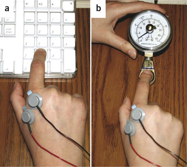
The black lead is over the dorsolateral aspect of this muscle's proximal tendon. The red lead is over the FDI mid-belly. The green rectangular lead is a ground over a bony aspect of the wrist. A red Velcro lead (not pictured), dipped in saline, is snug around the proximal arm. Subjects are trained on two different motor tasks for a total of 30 min. (a) The first task requires them to alternate between pressing keys 1 and 3 as fast as they can. (b) The second task requires them to press down on a hydraulic dynamometer pad once every 5 s holding 5 kg of force for 1 s.
-
22
Follow with the forced finger adduction task. For this, each subject must be seated with hand pronated upon the table, fingers in a relaxed position. Place the Jamar hydraulic dynamometer force transducer 2 cm medial (i.e., to the thumb side) from the index finger tip. Place a timer within the subject's view on the table and set for 5 min. Subjects should adduct their index finger to the transducer's force pad and press to a force of 5 kg (49 N) and hold for 1 s (Fig. 4b). Repeat every 5 s for 5 min, followed by a 2-min break.
-
23
Repeat Steps 21 and 22 such that each subject performs two trials of each task, for a total FDI training period of approximately 30 min.

Post-training TMS
-
24
Immediately after training, the subject, who has remained in the TMS stereotaxic apparatus with unmoved tracker glasses, should undergo the same TMS procedures that were used to generate the pre-training map (i.e., Steps 16–19 above). Again, in order to have the pre- and post-training TMS maps be directly comparable, the subject's trackers on headband or glasses cannot be adjusted in any way during either TMS session or during the training.
TMS data analysis
-
25
Measure peak-to-peak MEP amplitudes at each site offline using an EMG analysis program. Average amplitudes across the ten stimulation pulses for each positive site and record. Some authors prefer to measure the compound motor action potential (CMAP) and, for individual subjects, normalize mean MEP measures in relation to this to account for variability in peripheral nervous system measures such as muscle bulk39. This approach can be adopted if desired. Calculate map area by multiplying the number of positive (blue or green) sites by 1 cm2. Map volume should be expressed as the sum of the mean peak-to-peak MEP amplitudes generated within the map40. Center of gravity should be represented as an amplitude-weighted position and should be calculated as follows: for each positive TMS site on the map, the amplitude weight should be computed as the mean amplitude at that position divided by the sum of peak-to-peak MEP amplitudes recorded for the map. The weight at any stimulating position is interpreted as the proportion of the total map area contributed by that location40. For the recruitment curve data, MEP amplitude is plotted as a function of the four stimulus intensities (90, 110, 130 and 150% resting motor threshold). These data are then fitted to a linear model, and the slope is calculated; fitting to other models has also been suggested49. Mean amplitude of MEPs can also be normalized to pre-training levels to calculate the percentage change after training.
Troubleshooting
Step 15 It is critical that the subject registration in the neuronavigation program is done as precisely as possible. This is particularly important if the training whose effects are to be examined requires the subject to leave the lab and return, for example, several days later. Such careful registration helps to ensure that the stimulation sites are constant before and after training. Subjects should not remove, adjust or touch the tracking headband/glasses that hold the reflecting spheres at any time point, including during training, as it is critical to maintain a fixed spatial relationship between the subject's head and the headband/glasses22. Experimental protocols that are associated with any movement of the reflecting spheres relative to the head would require further measures to maintain this constant spatial relationship.
Step 16 Excessive noise may be observed in the EMG signal at the beginning of or during the mapping session. Room noise can be reduced by ensuring that non-essential equipment is unplugged or off. If the noise is severe, the electrodes and/or Velcro wraparound can be re-attached.
General Experience with the above methods yields several caveats that might be useful for consistently obtaining clean data. Similarly, surface EMG electrode placement over the FDI is also crucial and subjects should be warned to be very careful not to remove the electrodes during motor training.
The TMS coil should be regularly registered to the Brainsight system. Stimulation artifacts and recording noise should be carefully controlled with ground placement; in some cases, artifacts can be removed only by unplugging all electrical devices anywhere near the TMS apparatus. Because the normal latency from TMS pulse to first deflection for the FDI MEP is greater than 20 ms, the presence of any waveforms within 20 ms of the TMS pulse should not be included in the analysis of MEP amplitude. Repositioning or replacing the FDI recording electrodes during the experiment may cause some variation in MEP responses and should be avoided if possible. If needed, surgical tape can be applied over the electrodes to fix them in place and prevent them from coming off during the experiment. However, the saline-soaked Velcro wrap can be removed and re-soaked, for example, while the subject is being trained on the motor task, as this must remain wet throughout mapping. Doing so helps ensure a clean signal from the recording electrodes. In the rare case that a very large voltage waveform artifact appears, the MEP measurement is obscured. This is due to a TMS-generated voltage being conducted to the EMG leads through the skin rather than via the nervous system. This can be eliminated by replacing the electrodes, re-soaking the Velcro wrap in saline or applying a second saline-soaked Velcro wrap ground lead around the proximal arm to further ground the subject.
During mapping it is critical that the paddle is consistently held flat against the skull and at the proper (45°) angle from midline. Furthermore, while you are generating the recruitment curve, it is important to be sure that the TMS paddle is held in a fixed position over the SOLRMT. This can be achieved by locking Brainsight's mechanical arm used to hold the paddle.
Continued use of the TMS coil for extended time periods, especially at higher stimulation intensities, can cause the apparatus to overheat. When this arises, the machine is left on to permit the fan to cool it, but all stimulation is suspended until the unit returns to a suitable temperature. If this becomes a frequent issue for certain protocols, use of a coil that has a cooling vacuum connection attached can be considered.
The current protocol was designed with a specific manufacturer's components, as discussed above. The effect that varying MRI or TMS manufacturer has on results obtained with the current method has not been studied but is expected to be minimal.
Timing
MRI acquisition: approximately 20–30 min
Subject preparation and pre-training for TMS: 60 min, which with two investigators can be done in parallel with the 30–40 min of image processing/preparation
Pre-training TMS: 60 min
Motor training: 30 min
Post-training TMS: 45 min
The relationship that time to perform post-training TMS mapping has with the temporal characteristics of training effects must be considered. If a training procedure, or other plasticity-inducing experience, lasts only a few minutes, then the post-training TMS procedure must be modified. The length of time required for the post-training TMS procedure might need to be shortened in such a situation, and strict attention might need to be paid to the order with which TMS sites are stimulated.
Anticipated results
The approach described herein permits comparison of these TMS measures before and after training. In our experience, such measures have a normal distribution and can be analyzed with parametric statistics. Other TMS-based measures not described herein, such as latency and cortical excitability, can also be measured.
Several possible controls can be incorporated, depending upon study design. TMS can done twice, on a separate visit, with no training between TMS assessments. Alternatively, TMS can be done before and after a control-training experience that is not expected to change cortical maps. Another possible control would be to examine TMS maps, before and after training, for a second muscle not expected to change in relation to the training experience.
In healthy subjects, the resting motor threshold for FDI is usually approximately 40–50% of the TMS device output. MEP amplitudes are usually approximately 160 μV at 110%, 400 μV at 130% and 600 μV at 150% of the lowest motor resting threshold and increase in response to motor training (Fig. 5). The FDI map area is approximately 9 cm2 and map volume approximately 4.5 U pre-training. Post-training map area increases from 9 to approximately 13 cm2, and map volume increases from 4.5 to 6 U. The center of gravity should shift approximately 2.0 cm.

This curve is also known as an input–output curve and shows mean (±s.d.) motor evoked potential (MEP) amplitude in response to progressively higher stimulation levels. The x-axis is the input, which is percentage of the lowest resting motor threshold. The y-axis is the motor evoked potential amplitude in microvolts. Two input–output curves are presented from a healthy subject in relation to 30 min of training, one pre-training and one post-training. For each, a slope and a fit can be described.
References
Teskey, G., Monfils, M., VandenBerg, P. & Kleim, J. Motor map expansion following repeated cortical and limbic seizures is related to synaptic potentiation. Cereb. Cortex 12, 98–105 (2002).
Monfils, M.H., VandenBerg, P.M., Kleim, J.A. & Teskey, G.C. Long-term potentiation induces expanded movement representations and dendritic hypertrophy in layer V of rat sensorimotor neocortex. Cereb. Cortex 14, 586–593 (2004).
Pascual-Leone, A. et al. Study and modulation of human cortical excitability with transcranial magnetic stimulation. J. Clin. Neurophysiol. 15, 333–343 (1998).
Peinemann, A. et al. Long-lasting increase in corticospinal excitability after 1800 pulses of subthreshold 5 Hz repetitive TMS to the primary motor cortex. Clin. Neurophysiol. 115, 1519–1526 (2004).
Cramer, S. et al. Use of functional MRI to guide decisions in a clinical stroke trial. Stroke 36, e50–e52 (2005).
Stefan, K., Kunesch, E., Cohen, L.G., Benecke, R. & Classen, J. Induction of plasticity in the human motor cortex by paired associative stimulation. Brain 123 (Pt 3), 572–584 (2000).
Jacobs, K.M. & Donoghue, J.P. Reshaping the cortical motor map by unmasking latent intracortical connections. Science 251, 944–947 (1991).
Reis, J. et al. Modulation of human motor cortex excitability by single doses of amantadine. Neuropsychopharmacology 31, 2758–2766 (2006).
Charlton, C.S., Ridding, M.C., Thompson, P.D. & Miles, T.S. Prolonged peripheral nerve stimulation induces persistent changes in excitability of human motor cortex. J. Neurol. Sci. 208, 79–85 (2003).
Keller, A., Weintraub, N.D. & Miyashita, E. Tactile experience determines the organization of movement representations in rat motor cortex. Neuroreport 7, 2373–2378 (1996).
Brasil-Neto, J. et al. Rapid modulation of human cortical motor outputs following ischaemic nerve block. Brain 116 (Pt 3), 511–525 (1993).
Kleim, J., Barbay, S. & Nudo, R.J. Functional reorganization of the rat motor cortex following motor skill learning. J. Neurophysiol. 80, 3321–3325 (1998).
Jensen, J.L., Marstrand, P.C. & Nielsen, J.B. Motor skill training and strength training are associated with different plastic changes in the central nervous system. J. Appl. Physiol. 99, 1558–1568 (2005).
Kleim, J.A. et al. BDNF val66met polymorphism is associated with modified experience-dependent plasticity in human motor cortex. Nat. Neurosci. 9, 735–737 (2006).
Pascual-Leone, A. et al. Modulation of muscle responses evoked by transcranial magnetic stimulation during the acquisition of new fine motor skills. J. Neurophysiol. 74, 1037–1045 (1995).
Monfils, M.H., Plautz, E.J. & Kleim, J.A. In search of the motor engram: motor map plasticity as a mechanism for encoding motor experience. Neuroscientist 11, 471–483 (2005).
Classen, J., Liepert, J., Wise, S.P., Hallett, M. & Cohen, L.G. Rapid plasticity of human cortical movement representation induced by practice. J. Neurophysiol. 79, 1117–1123 (1998).
Meintzschel, F. & Ziemann, U. Modification of practice-dependent plasticity in human motor cortex by neuromodulators. Cereb. Cortex 16, 1106–1115 (2006).
Kleim, J.A. et al. Cortical synaptogenesis and motor map reorganization occur during late, but not early, phase of motor skill learning. J. Neurosci. 24, 628–633 (2004).
Nudo, R.J., Milliken, G.W., Jenkins, W.M. & Merzenich, M.M. Use-dependent alterations of movement representations in primary motor cortex of adult squirrel monkeys. J. Neurosci. 16, 785–807 (1996).
Paus, T. & Wolforth, M. Transcranial magnetic stimulation during PET: reaching and verifying the target site. Hum. Brain Mapp. 6, 399–402 (1998).
Gugino, L.D. et al. Transcranial magnetic stimulation coregistered with MRI: a comparison of a guided versus blind stimulation technique and its effect on evoked compound muscle action potentials. Clin. Neurophysiol. 112, 1781–1792 (2001).
Neggers, S.F. et al. A stereotactic method for image-guided transcranial magnetic stimulation validated with fMRI and motor-evoked potentials. Neuroimage 21, 1805–1817 (2004).
Kleim, J.A., Jones, T.A. & Schallert, T. Motor enrichment and the induction of plasticity before or after brain injury. Neurochem. Res. 28, 1757–1769 (2003).
Cramer, S. Clinical issues in animal models of stroke and rehabilitation. ILAR J. 44, 83–84 (2003).
Nudo, R.J. Functional and structural plasticity in motor cortex: implications for stroke recovery. Phys. Med. Rehabil. Clin. N. Am. 14 (1 Suppl) S57–S76 (2003).
Oldfield, R.C. The assessment and analysis of handedness: the Edinburgh Inventory. Neuropsychologia 9, 97–113 (1971).
Pascual-Leone, A., Davey, N.J., Rothwell, J., Wassermann, E.M. & Basant, K. Handbook of Transcranial Magnetic Stimulation (Arnold, New York, 2002).
Keel, J.C., Smith, M.J. & Wassermann, E.M. A safety screening questionnaire for transcranial magnetic stimulation. Clin. Neurophysiol. 112, 720 (2001).
Wassermann, E.M. Risk and safety of repetitive transcranial magnetic stimulation: report and suggested guidelines from the International Workshop on the Safety of Repetitive Transcranial Magnetic Stimulation, June 5–7, 1996. Electroencephalogr. Clin. Neurophysiol. 108, 1–16 (1998).
Rothwell, J.C. et al. Magnetic stimulation: motor evoked potentials. The International Federation of Clinical Neurophysiology. Electroencephalogr. Clin. Neurophysiol. Suppl. 52, 97–103 (1999).
Tranulis, C. et al. Motor threshold in transcranial magnetic stimulation: comparison of three estimation methods. Neurophysiol. Clin. 36, 1–7 (2006).
Schutter, D.J. & van Honk, J. A standardized motor threshold estimation procedure for transcranial magnetic stimulation research. J. ECT 22, 176–178 (2006).
Claus, D., Murray, N.M., Spitzer, A. & Flugel, D. The influence of stimulus type on the magnetic excitation of nerve structures. Electroencephalogr. Clin. Neurophysiol. 75, 342–349 (1990).
Maccabee, P.J. et al. Influence of pulse sequence, polarity and amplitude on magnetic stimulation of human and porcine peripheral nerve. J. Physiol. 513 (Pt 2), 571–585 (1998).
Ono, M., Kubik, S. & Abernathey, C. Atlas of the Cerebral Sulci (G. Thieme Verlag, Stuttgart, 1990).
Brasil-Neto, J.P., McShane, L.M., Fuhr, P., Hallett, M. & Cohen, L.G. Topographic mapping of the human motor cortex with magnetic stimulation: factors affecting accuracy and reproducibility. Electroencephalogr. Clin. Neurophysiol. 85, 9–16 (1992).
Perotto, A. Anatomical Guide for the Electromyographer. The Limbs and Trunk (Charles C. Thomas, Springfield, Illinois, 1994).
Talleli, P., Greenwood, R.J. & Rothwell, J.C. Arm function after stroke: neurophysiological correlates and recovery mechanisms assessed by transcranial magnetic stimulation. Clin. Neurophysiol. 117, 1641–1659 (2006).
Wolf, S.L. et al. Intra-subject reliability of parameters contributing to maps generated by transcranial magnetic stimulation in able-bodied adults. Clin. Neurophysiol. 115, 1740–1747 (2004).
Yousry, T. et al. Localization of the motor hand area to a knob on the precentral gyrus. A new landmark. Brain 120, 141–157 (1997).
Boroojerdi, B. et al. Localization of the motor hand area using transcranial magnetic stimulation and functional magnetic resonance imaging. Clin. Neurophysiol. 110, 699–704 (1999).
Rosenkranz, K. & Rothwell, J.C. Differential effect of muscle vibration on intracortical inhibitory circuits in humans. J. Physiol. 551, 649–660 (2003).
Wassermann, E.M. Variation in the response to transcranial magnetic brain stimulation in the general population. Clin. Neurophysiol. 113, 1165–1171 (2002).
Rossini, P.M. et al. Non-invasive electrical and magnetic stimulation of the brain, spinal cord and roots: basic principles and procedures for routine clinical application. Report of an IFCN committee. Electroencephalogr. Clin. Neurophysiol. 91, 79–92 (1994).
Penfield, W. & Boldrey, E. Somatic motor and sensory representation in the cerebral cortex of man as studied by electrical stimulation. Brain 60, 389–443 (1937).
Cramer, S.C. & Crafton, K.R. Somatotopy and movement representation sites following cortical stroke. Exp. Brain Res. 168, 25–32 (2006).
Helmich, R.C., Baumer, T., Siebner, H.R., Bloem, B.R. & Munchau, A. Hemispheric asymmetry and somatotopy of afferent inhibition in healthy humans. Exp. Brain Res. 167, 211–219 (2005).
Devanne, H., Lavoie, B.A. & Capaday, C. Input-output properties and gain changes in the human corticospinal pathway. Exp. Brain Res. 114, 329–338 (1997).
Acknowledgements
We thank Steven Wolf, Emory University; Elizabeth Orr, Daniel Ro, Vu Le, Sheila Chan, University of California Irvine; Kellan Schallart, University of Texas; Sarah McCann, Malcolm Randall VA Hospital, Gainesville, Florida. Studies were carried out in the General Clinical Research Center of the University of California, Irvine, with funds provided by the National Center for Research Resources, 5M01RR 00827-29, NS-45563, U.S. Public Health Service.
Author information
Authors and Affiliations
Corresponding author
Ethics declarations
Competing interests
The authors declare no competing financial interests.
Rights and permissions
About this article
Cite this article
Kleim, J., Kleim, E. & Cramer, S. Systematic assessment of training-induced changes in corticospinal output to hand using frameless stereotaxic transcranial magnetic stimulation. Nat Protoc 2, 1675–1684 (2007). https://doi.org/10.1038/nprot.2007.206
Published:
Issue Date:
DOI: https://doi.org/10.1038/nprot.2007.206
This article is cited by
-
Precise motor mapping with transcranial magnetic stimulation
Nature Protocols (2023)
-
Reliability of active robotic neuro-navigated transcranial magnetic stimulation motor maps
Experimental Brain Research (2023)
-
Intensity matters: protocol for a randomized controlled trial exercise intervention for individuals with chronic stroke
Trials (2022)
-
Examining the role of the supplementary motor area in motor imagery-based skill acquisition
Experimental Brain Research (2021)
-
Simultaneous Recording of Motor Evoked Potentials in Hand, Wrist and Arm Muscles to Assess Corticospinal Divergence
Brain Topography (2021)
Comments
By submitting a comment you agree to abide by our Terms and Community Guidelines. If you find something abusive or that does not comply with our terms or guidelines please flag it as inappropriate.
