
Abstract
The generation, manipulation and fundamental understanding of entanglement lies at very heart of quantum mechanics. Among various types of entangled states, the NOON states are a kind of special quantum entangled states with two orthogonal component states in maximal superposition, which have a wide range of potential applications in quantum communication and quantum information processing. Here, we propose a fast and simple scheme for generating NOON states of photons in two superconducting resonators by using a single superconducting transmon qutrit. Because only one superconducting qutrit and two resonators are used, the experimental setup for this scheme is much simplified when compared with the previous proposals requiring a setup of two superconducting qutrits and three cavities. In addition, this scheme is easier and faster to implement than the previous proposals, which require using a complex microwave pulse, or a small pulse Rabi frequency in order to avoid nonresonant transitions.
Introduction
VArious physical systems have been considered for building up quantum information processors. Among them, circuit QED consisting of microwave resonators and superconducting qubits is particularly appealing1,2. Superconducting qubits (such as charge, flux and transmon qubits) behave as artificial atoms, they have relatively long decoherence times3,4,5,6,7 and various single- and multiple-qubit operations with state readout have been demonstrated8,9,10,11,12. On the other hand, a superconducting resonator provides a quantized cavity field which acts as a quantum bus and thus can mediate long-distance and strong interaction between distant superconducting qubits13,14,15. Furthermore, the strong coupling between a microwave cavity and superconducting charge qubits16 or flux qubits17 was earlier predicated in theory and has been experimentally demonstrated18,19. Because of these features, circuit QED has been widely utilized for quantum information processing. During the past decade, based on circuit QED, many theoretical proposals have been presented for the preparation of Fock states, coherent states, squeezed states, Schördinger Cat states and arbitrary superpositions of Fock states of a single superconducting resonator20,21,22. So far, Fock states and their superpositions of a resonator have been experimentally produced by using a superconducting qubit23,24,25.
Intense effort has been recently devoted to the preparation of entangled states of photons in two or more superconducting resonators26,27,28,29. The NOON states are a special type of photonic entangled states with two orthogonal component states in maximal superposition, which play the crucial role in quantum optical lithography30,31, quantum metrology32,33,34,35, precision measurement of transmons36,37,38 and quantum information processing39,40.
In Ref. 26, a theoretical method for synthesizing an arbitrary quantum state of two superconducting resonators using a tunable superconducting qubit has been proposed. This method is based on alternative resonant interactions of the coupler qubit with two cavity modes and a classical pulse. As pointed out in26, the Rabi frequency of the classical pulse needs to be much smaller than the photon-number-dependent Stark shifts induced by dispersive interaction with the two field modes and, hence, the pulse can drive the qubit to undergo a rotation conditional upon the state of the cavity modes. This implies that the time needed to complete the rotation in each step should be much (two orders of magnitude) longer than the vacuum Rabi period of the coupled qubit-resonator system.
In Ref. 27, the authors proposed a theoretical scheme for creating NOON states of two resonators, which was implemented in experiments for N ≤ 3 by H. Wang et al.28. The method in27,28 operates essentially by employing two three-level superconducting qutrits as couplers, preparing them in a Bell state and then performing N steps of operation to swap the coherence of the Bell state onto the two resonators through a sequence of classical pulses applied to the two coupler qutrits. In addition, as discussed in27,28, a third resonator or cavity is needed in order to prepare the two coupler qutrits in the Bell state.
Ref. 29 presented an approach to control the quantum state of two superconducting resonators using a complicated classical microwave pulse. For the generation of NOON states, this scheme also requires two superconducting qubits which are initially prepared in a Bell state. Another problem is that the produced state is essentially an entangled state of two resonators and two qubits. To obtain the pure photonic NOON state, one should use additional techniques to decouple the qubits from the resonators.
As reported in28, the fidelity of the obtained NOON state decreases dramatically with the photon number N due to decoherence, dropping to 0.33 for N = 3. In order to be useful in quantum technologies, the fidelity needs to be significantly improved. Thus, it is worthy of exploring more efficient schemes to generate the NOON states with a higher fidelity.
In this work, we propose an alternative scheme for generating the NOON state of two resonators coupled to a superconducting transmon qutrit, via resonant interactions. This proposal has the following advantages: (i) Because of using only one superconducting qutrit and two resonators, the experimental setup is greatly simplified when compared with that in27,28,29, which is important for decreasing decoherence effects; (ii) In principle, there is no limitation on the intensity of the classical pulse for our scheme and thus the operation can be performed much faster when compared with the method in26. Overall, the important features of our scheme are simplicity, rapidness and robustness.
We will also give a detailed discussion of the experimental issues and then analyze the possible experimental implementation. Our numerical simulation shows that a high-fidelity generation of the NOON state with N ≤ 3 is feasible within the present circuit QED technique.
Results
Noon-state preparation
Consider two resonators coupled to a superconducting transmon qutrit (Fig. 1). The three ladder-type levels of the qutrit are labeled as |g〉, |e〉 and |f〉 with energy Eg < Ee < Ef. Suppose that the coupler qutrit is initially in the state  and the two resonators are initially in the vacuum state |0〉a |0〉b. The qutrit can be made to be decoupled from the two resonators by a prior adjustment of the qutrit level spacings. Note that for superconducting transmon qutrits, the level spacings can be rapidly adjusted by varying external control parameters (e.g., magnetic flux applied to superconducting quantum interference device (SQUID) loops of two-junction transmon qutrits; see, e.g.41,42,43).

Setup for two resonators a and b coupled by a superconducting transmon qutrit.
Each resonator here is a one-dimensional coplanar waveguide transmission line resonator. The circle A represents a superconducting transmon qutrit, which is capacitively coupled to each resonator via a capacitance Cc.
For simplicity, we define ωeg (ωfe) as the |g〉 ↔ |e〉 (|e〉 ↔ |f〉) transition frequency of the qutrit and Ωeg (Ωfe) as the Rabi frequency of the classical pulse driving the coherent |g〉 ↔ |e〉 (|e〉 ↔ |f〉) transition. In addition, the frequency, initial phase and duration of the microwave pulse are denoted as {ω, ϕ, t} in the rest of the paper.
The procedure for generating the NOON state of photons in the two resonators contains 2N steps. We assume that resonator b (a) is decoupled from the qutrit during each of the first (second) N steps due to large detunings, which can be achieved by prior adjustment of the resonator frequency. The effects of off-resonant qutrit-resonator couplings and classical drivings on the fidelity of the prepared state will be taken into account later.
Before the operations for the first N steps, we need to adjust the level spacings of the qutrit such that resonator a is resonant with the |g〉 ↔ |e〉 transition, but is far off-resonant with (decoupled from) the |e〉 ↔ |f〉 transition so that the coupling between resonator a and the |e〉 ↔ |f〉 transition can be neglected [Fig. 2(a)]. Meanwhile, resonator b is far off-resonant with both of these two transitions and thus it is unaffected during this interaction (i.e., resonator b is decoupled from the qutrit). Under these conditions, the state |f〉 remains unchanged due to the large detuning. In the interaction picture with respect to the free Hamiltonian of the whole system, the Hamiltonian describing this operation is given by  , where a+ is the photon creation operator of the mode of resonator a and geg is the coupling constant between the mode of the resonator a and the |g〉 ↔ |e〉 transition [Fig. 2(a)].

(a) Resonator a is far-off resonant with the |e〉 ↔ |f〉 transition but resonant with the |g〉 ↔ |e〉 transition. (b) The pulse is far-off resonant with the |e〉 ↔ |f〉 transition but resonant with the |g〉 ↔ |e〉 transition. (c) Resonator b is far-off resonant with the |g〉 ↔ |e〉 transition but resonant with the |e〉 ↔ |f〉 transition. (d) The pulse is far-off resonant with the |g〉 ↔ |e〉 transition but resonant with the |e〉 ↔ |f〉 transition.
The operations of the first N steps are described below:
Step 1: Let resonator a resonant with the |g〉 ↔ |e〉 transition. Under the Hamiltonian HI, the state component |f〉 |0〉a is not changed because of HI |f〉 |0〉a = 0, while |e〉 |0〉a undergoes the Jaynes-Cumming evolution44. After an interaction time t1 = π/(2geg) (i.e., half a Rabi oscillation), the state |e〉 |0〉a changes to −i |g〉 |1〉a (for the details, see the discussion in the part of Methods below). Hence, the initial state  of the whole system becomes

Then, apply a microwave pulse of {ωeg, −π/2, π/(2Ωeg)} to the qutrit to pump the state |g〉 back to |e〉 [Fig. 2(b)], transforming the state (1) to

Here and below, we assume  so that the interaction between the qutrit and resonotor a is negligible during the application of this pulse.
Step j (j = 2, 3, …,N − 1): Repeat the operation of step 1. The time for the qutrit interacting with resonator a is set by  (i.e., half a Rabi oscillation). After an interaction time tj, the state |f〉 |0〉a remains unchanged while the state |e〉 |j − 1〉a changes to −i |g〉 |j〉a, which further changes to −i |e〉 |j〉a due to a microwave pulse of {ωeg, −π/2, π/(2Ωeg)} pumping the state |g〉 back to |e〉. Hence, one can easily verify that after the operation of steps (2, 3, …, N − 1), the state (2) becomes

Step N: Let resonator a resonant with the |g〉 ↔ |e〉 transition for an interaction time  [Fig. 2(a)]. As a result, we have the transformation |e〉 |N − 1〉a → −i |g〉 |N〉a while the state |f〉 |0〉a remains unchanged. Thus, the state (3) becomes

In above we have given a detailed description of the operations for the first N steps. Now let us give a description on the second N steps. To begin with, we need to adjust the level spacings of the qutrit to bring resonator b resonant with the |e〉 ↔ |f〉 transition but far off-resonant with the |g〉 ↔ |e〉 transition [Fig. 2(c)]. On the other hand, resonator a is far off-resonant with each transition so that it is unaffected during this interaction (i.e., resonator a is decoupled from the qutrit, which can be achieved by adjusting the frequency of resonator a). In the interaction picture with respect to the free Hamiltonian of the whole system, the Hamiltonian governing this operation is given by  , where b+ is the photon creation operator of the mode of resonator b and gfe is the coupling constant between the resonator b and the |e〉 ↔ |f〉 transition [Fig. 2(c)].
Since the level spacings of the qutrit are now different from those used in the operation of the first N steps, we now define  ,
,  and
and  as the |g〉 ↔ |e〉 transition frequency, the |e〉 ↔ |f〉 transition frequency and the |g〉 ↔ |f〉 transition frequency of the qutrit, respectively.
The operations of the second N steps are as follows:
Step 1: Let resonator b resonant with the |e〉 ↔ |f〉 transition [Fig. 2(c)]. Under the Hamiltonian HI, the state component |g〉 |0〉b does not change because of HI |g〉 |0〉b = 0, while |f〉 |0〉b undergoes the Jaynes-Cumming evolution. After an interaction time  , the state |f〉 |0〉b changes to −i |e〉 |1〉b (see the discussion in the Methods below). Thus, one can see that the state (4) changes to

Then, apply a microwave pulse of  to the qutrit to pump the state |e〉 back to |f〉 [Fig. 2(d)], transforming the state (5) to

Here and below, we assume  such that the qutrit-resonator coupling is negligible during the application of this pulse.
Step j (j = 2, 3, …, N − 1): Repeat the operation of step 1. The time for the qutrit interacting with resonator b is set by  . After an interaction time
  , the state |g〉 |0〉b remains unchanged while the state |f〉 |j − 1〉b changes to −i |e〉 |j〉b, which further turns into −i |f〉 |j〉b because of a microwave pulse of
  pumping the state |e〉 back to |f〉. After step N − 1, the state (6) becomes

Step N: Apply a microwave pulse of  to the qutrit to pump the state |g〉 back to |e〉 [note that in Fig. 2(d), the pulse is now resonant to the |g〉 ↔ |e〉 transition, instead of the |e〉 ↔ |f〉 transition]. To neglect the qutrit-resonator coupling during this pulse, the condition
  needs to be satisfied. Then, let resonator b resonant with the |e〉 ↔ |f〉 transition for an interaction time
  [Fig. 2(c)], leading to the transformation |f〉 |N − 1〉b → −i |e〉 |N〉b. Meanwhile, resonator a remains decoupled from the qutrit. As a result, the state (7) changes to

Then, adjust the level spacings of the qutrit back to the original level configuration such that the qutrit is decoupled from the two resonators. The result (8) shows that the two resonators a and b are prepared in a NOON state of photons, which are disentangled from the qutrit.
Previously we have assumed that during the first (second) N steps of operations, the resonator b (a) is decoupled from the qutrit. In principle, this requirement can be met by adjusting the level spacings of the qutrit41,42,43 or the resonator mode frequency such that the irrelevant resonator during the operation is highly detuned from the transition between any two levels of the coupler qutrit. The rapid tuning of cavity frequencies has been demonstrated in superconducting microwave cavities (e.g., in less than a few nanoseconds for a superconducting transmission line resonator45).
As shown above, our NOON-state preparation is based on the following approximations. For the first N steps of operation, we have neglected the off-resonant interaction between resonator a and the |e〉 ↔ |f〉 transition of the qutrit, the off-resonant interaction between the pulse and the |e〉 ↔ |f〉 transition of the qutrit and the off-resonant coupling of resonator b with the transition between any two levels of the qutrit. For the second N steps of operation, we have omitted the off-resonant interaction between resonator b and the |g〉 ↔ |e〉 transition of the qutrit, the off-resonant interaction between the pulse and the |g〉 ↔ |e〉 transition of the qutrit and the off-resonant coupling of resonator a with the transition between any two levels of the qutrit. In addition, for each step of operation, there exists an inter-cavity cross coupling, which was also not considered in our NOON-state preparation above. To quantify how well our protocol works out, later we will perform a numerical simulation for N ≤ 5, by taking all these effects into account.
Experimental issues
For the method to work the primary considerations shall be given to:
-
i
The total operation time τ, given by
(where td ~ 1–3 ns is the typical time required for adjusting the qutrit level spacings), needs to be much shorter than the energy relaxation time T1
 and dephasing time T2
 of the level |f〉 (|e〉) of the qutrit, such that decoherence caused by energy relaxation and dephasing of the qutrit is negligible for the operation. Note that
  and
and  of the qutrit are comparable to T1 and T2, respectively. For instance,
  and
and  for transmon qutrits.
 -
ii
For resonator k (k = a, b), the lifetime of the resonator mode is given by
 , where Qk, νk and
  are the (loaded) quality factor, frequency and the average photon number of resonator k, respectively. For the two resonators, the lifetime of entanglement of the resonator modes is given by
which should be much longer than τ, such that the effect of resonator decay is negligible during the operation.
-
iii
The inter-cavity cross coupling between the two resonators is determined mostly by the coupling capacitance Cc and the qutrit's self capacitance Cq, because the field leakage through space is extremely low for high-Q resonators as long as the inter-cavity distance is much greater than transverse dimension of the cavities - a condition easily met in experiments for the two resonators. Furthermore, as the result of our numerical simulation shown below (see Fig. 4), the effects of the inter-cavity coupling can however be made negligible as long as the corresponding inter-cavity coupling constant gab between resonators a and b is sufficiently small.
Figure 4 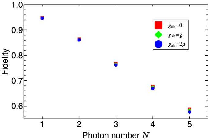
Fidelity versus N.
Refer to the text for the parameters used in the numerical calculation. For N = 1, 2, 3, 4, 5 and gab = 2 g, the fidelities are ~0.947, 0.861, 0.762, 0.669, 0.577, respectively.

 and dephasing time T2
 of the level |f〉 (|e〉) of the qutrit, such that decoherence caused by energy relaxation and dephasing of the qutrit is negligible for the operation. Note that
  and
and  of the qutrit are comparable to T1 and T2, respectively. For instance,
  and
and  for transmon qutrits.
  , where Qk, νk and
  are the (loaded) quality factor, frequency and the average photon number of resonator k, respectively. For the two resonators, the lifetime of entanglement of the resonator modes is given by

Fidelity
Hereafter, we give a discussion of the fidelity of the prepared NOON state for N ≤ 5.
The first N steps above for creating the NOON state involves the following two basic types of interactions:
-
i
The first one is the resonant coupling between resonator a and the |g〉 ↔ |e〉 transition. When the interaction between resonator a and the |e〉 ↔ |f〉 transition [Fig. 3(a)], the coupling between resonator b and the qutrit [Fig. 3(a)] and the inter-cavity crosstalk between the two resonators are taken into account, the corresponding interaction Hamiltonian is thus given by
Figure 3 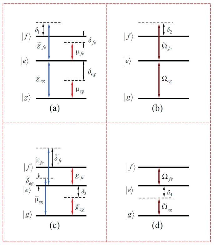
(a) and (c) Illustration of qutrit-resonator interactions. (b) and (d) Illustration of qutrit-pulse interactions. In (a), resonator a is resonant to the |g〉 ↔ |e〉 transition with coupling constant geg, while off-resonant to the |e〉 ↔ |f〉 transition with coupling constant
 and detuning δ1 = ωfe − ωa < 0; resonator b is off-resonant to the |g〉 ↔ |e〉 transition with coupling constant μeg and detuning δeg = ωeg − ωb > 0 and off-resonant to the |e〉 ↔ |f〉 transition with coupling constant μfe and detuning δfe = ωfe − ωb > 0. In (c), resonator b is resonant to the |e〉 ↔ |f〉 transition with coupling constant gfe, while off-resonant to the |g〉 ↔ |e〉 transition with coupling constant
  and detuning
  ; resonator a is off-resonant to the |g〉 ↔ |e〉 transition with coupling constant
  and detuning
  and off-resonant to the |e〉 ↔ |f〉 transition with coupling constant
  and detuning
  . In (b), a pulse (with frequency ω = ωeg) is resonant to the |g〉 ↔ |e〉 transition with Rabi frequency Ωeg, but off-resonant to the |e〉 ↔ |f〉 transition with Rabi frequency
  and detuning δ2 = ωfe − ω = ωfe − ωeg < 0. In (d), a pulse (with frequency
  ) is resonant to the |e〉 ↔ |f〉 transition with Rabi frequency Ωfe, but off-resonant to the |g〉 ↔ |e〉 transition with Rabi frequency
  and detuning
  . The qutrit-resonator interactions during the pulses of (b) and (d) are the same as those shown in (a) and (c), respectively and have been taken into account in the numerical simulation. Here, δ1 = δ2 because of ω = ωa and δ3 = δ4 due to ω = ωb.
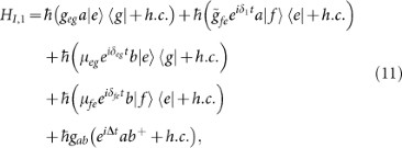
where the first term represents the resonant interaction of resonator a with the |g〉 ↔ |e〉 transition, while the second term represents the unwanted off-resonant coupling between resonator a and the |e〉 ↔ |f〉 transition with coupling constant
 and detuning δ1 = ωfe − ωa < 0 [Fig. 3(a)]. In addition, the third term represents the unwanted off-resonant coupling between resonator b and the |g〉 ↔ |e〉 transition with coupling constant μeg and detuning δeg = ωeg − ωb > 0 [Fig. 3(a)], while the fourth term represents the unwanted off-resonant coupling between resonator b and the |e〉 ↔ |f〉 transition with coupling constant μfe and detuning δfe = ωfe − ωb > 0 [Fig. 3(a)]. Finally, the last term indicates the inter-cavity crosstalk between the two resonators, where Δ = ωb − ωa < 0 is the detuning between the two resonators. The Hamiltonian HI,1 here, together with HI,2, HI,3 and HI,4 below, is written in the interaction picture with respect to the free Hamiltonian of the whole system.
 -
ii
The second one corresponds to the application of the pulse with {ωeg, −π/2, π/(2Ωeg)} to the qutrit. The interaction Hamiltonian governing this basic operation is given by

where the first term represents the resonant interaction of the pulse with the |g〉 ↔ |e〉 transition, while the second one represents the unwanted off-resonant coupling between the pulse and the |e〉 ↔ |f〉 transition with Rabi frequency
 and detuning δ2 = ωfe − ωeg < 0 [Fig. 3(b)]. Here, HI,1 is the Hamiltonian given in Eq. (11), describing the coupling between resonator a and the qutrit, the coupling between resonator b and the qutrit, as well as the inter-cavity crosstalk between the two resonators during the pulse.
 The second N steps above for creating the NOON state covers the following two basic types of interactions:
-
iii
The third one corresponds to the resonant coupling between the resonator b and the |e〉 ↔ |f〉 transition. When the unwanted off-resonant coupling between this resonator and the |g〉 ↔ |e〉 transition [Fig. 3(c)], the coupling between resonator a and the qutrit [Fig. 3(c)] and the inter-cavity crosstalk between the two resonators are considered, the total interaction Hamiltonian reads

where the first term represents the resonant interaction of resonator b with the |e〉 ↔ |f〉 transition, while the second term represents the unwanted off-resonant coupling between resonator b and the |g〉 ↔ |e〉 transition with coupling constant
 and detuning
 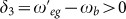 [Fig. 3(c)]. In addition, the third term represents the unwanted off-resonant coupling between resonator a and the |g〉 ↔ |e〉 transition with coupling constant
  and detuning
  [Fig. 3(c)], while the fourth term represents the unwanted off-resonant coupling between resonator a and the |e〉 ↔ |f〉 transition with coupling constant
  and detuning
 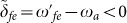 [Fig. 3(c)].
 -
iv
The last one is the pump of the qutrit with the pulse
 , with the interaction Hamiltonian described by
where the first term denotes the resonant pump of the |e〉 ↔ |f〉 transition, while the second one represents the unwanted off-resonant excitation of the |g〉 ↔ |e〉 transition with Rabi frequency
 and detuning
 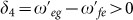 [Fig. 3(d)]. Here, HI,3 is the Hamiltonian given in Eq. (13), describing the coupling between resonator a and the qutrit, the coupling between resonator b and the qutrit, as well as the inter-cavity crosstalk between the two resonators during the pulse.

 and detuning δ1 = ωfe − ωa < 0; resonator b is off-resonant to the |g〉 ↔ |e〉 transition with coupling constant μeg and detuning δeg = ωeg − ωb > 0 and off-resonant to the |e〉 ↔ |f〉 transition with coupling constant μfe and detuning δfe = ωfe − ωb > 0. In (c), resonator b is resonant to the |e〉 ↔ |f〉 transition with coupling constant gfe, while off-resonant to the |g〉 ↔ |e〉 transition with coupling constant
  and detuning
  ; resonator a is off-resonant to the |g〉 ↔ |e〉 transition with coupling constant
  and detuning
  and off-resonant to the |e〉 ↔ |f〉 transition with coupling constant
  and detuning
  . In (b), a pulse (with frequency ω = ωeg) is resonant to the |g〉 ↔ |e〉 transition with Rabi frequency Ωeg, but off-resonant to the |e〉 ↔ |f〉 transition with Rabi frequency
  and detuning δ2 = ωfe − ω = ωfe − ωeg < 0. In (d), a pulse (with frequency
  ) is resonant to the |e〉 ↔ |f〉 transition with Rabi frequency Ωfe, but off-resonant to the |g〉 ↔ |e〉 transition with Rabi frequency
  and detuning
  . The qutrit-resonator interactions during the pulses of (b) and (d) are the same as those shown in (a) and (c), respectively and have been taken into account in the numerical simulation. Here, δ1 = δ2 because of ω = ωa and δ3 = δ4 due to ω = ωb.
 and detuning δ1 = ωfe − ωa < 0 [
 and detuning δ2 = ωfe − ωeg < 0 [
 and detuning
  [
[ and detuning
  [
[ and detuning
  [
[ , with the interaction Hamiltonian described by
 and detuning
  [
[It is noted that the term describing the pulse- or resonator-induced coherent |g〉 ↔ |f〉 transition for the qutrit is not included in the Hamiltonians HI,1, HI,2HI,3 and HI,4, since the error caused by this transition is much smaller than those described above. This is because: (i) the two resonators and the pulses are highly detuned from the |g〉 ↔ |f〉 transition with the relevant detunings being much larger than those for the |g〉 ↔ |e〉 and |e〉 ↔ |f〉 transitions,  (Fig. 3); and (ii) for a transmon qutrit with the three levels considered here, the |g〉 ↔ |f〉 dipole matrix element is much smaller than that of the |g〉 ↔ |e〉 and |e〉 ↔ |f〉 transitions46.
When the dissipation and dephasing are included, the dynamics for the kth type of interactions is determined by the following master equation

where HI,k for k = 1, 2, 3 and 4 are the above Hamiltonians HI,1, HI,2, HI,3 and HI,4, respectively;  (with Λ = a, b, S−,fe, S−,eg), S−,fe = |e〉 〈f|, S−,eg = |g〉 〈e|, Sff = |f〉 〈f| and See = |e〉 〈e|. In addition, κa (κb) is the decay rate of the resonator mode a (b); γfe is the energy relaxation rate for the level |f〉 associated with the decay path |f〉 → |e〉; γeg is that for the level |e〉; and γϕ,f (γϕ,e) is the dephasing rate of the level |f〉 (|e〉).
The fidelity of the whole operation is given by  , where |ψid〉 is the output state given in Eq. (8) for an ideal system (i.e., without unwanted couplings, dissipation and dephasing) after the entire operation, while
  is the final density operator of the whole system when the operations are performed in a realistic physical system.
We now numerically calculate the fidelity of the NOON state prepared above, with N ≤ 5. For simplicity, we set: (i) δ1/(2π) = δ2/(2π) = −400 MHz and δ3/(2π) = δ4/(2π) = 400 MHz43, (ii) Ωeg = Ωfe = Ω (achievable via adjusting the pulse intensities), thus  and
and  for the transmon qutrit here46; (iii)
  and thus
  46. In addition, μeg, μfe,
  and
and  can be determined due to
  ,
,  ,
,  and
and  . For superconducting transmon qutrits, the typical transition frequency between two neighbor levels is between 5 and 10 GHz. As an example, let us consider resonator a with frequency ωa/(2π) ~ 6 GHz while resonator b with frequency ωb/(2π) ~ 3.5 GHz. Other parameters used in the numerical calculation are as follows: (i) Δ/(2π) = −2.5 GHz, (ii) Ω/(2π) = 18 MHz47,48), (iii)
  ,
,  ,
,  (which are available in experiment42) and (iv)
  . For the parameters chosen here, the fidelity for N ≤ 5 is shown in Fig. 4 for gab = 0, g and 2 g. Fig. 4 was plotted by numerically optimizing the coupling constants, e.g., g/(2π) = 3.9, 2.2, 1.8, 1.5, 1.3 MHz for N = 1, 2, 3, 4, 5, respectively. The coupling strengths with these values are readily achievable in experiment because g/(2π) ~ 220 MHz has been reported for a superconducting transmon qubit coupled to a one-dimensional standing-wave CPW (coplanar waveguide) resonator49. It can be seen from Fig. 4 that when gab ≤ 2 g, the effect of the inter-cavity coupling is negligible and a high fidelity
  can be obtained for N ≤ 3.
The fidelity can be further increased by improving the system parameters. For instance, Fig. 5 shows that the fidelity for N = 3 can be increased to ~ 85% for  ,
,  and
and  , which can be reached in the near future due to the rapid development of the circuit-QED techniques (e.g., decoherence time ~ 10 μs has been demonstrated in a superconducting transmon qubit coupled to a 3D cavity50).

Fidelity versus {T, g} for N = 3.
The plot was drawn by setting  ,
,  ,
,  . Other parameters used in the numerical simulation are the same as those used in Fig. 4.
For the resonators a and b of frequencies given above and the  and
and  used in the numerical calculation, the required quality factors for the two resonators are Qa ~ 7.5 × 10⁵ and Qb ~ 4.4 × 10⁵. Note that superconducting CPW resonators with a loaded quality factor Q ~ 106 have been experimentally demonstrated51,52 and planar superconducting resonators with internal quality factors above one million (Q > 106) have also been reported recently53. Our analysis given here demonstrates that high-fidelity generation of the NOON state with N ≤ 3 using the present proposal is possible within the present circuit QED techniques.
The condition, gab ≤ 2 g, is not difficult to satisfy with typical capacitive cavity-qutrit coupling illustrated in Fig. 1. As discussed in54, as long as the cavities are physically well separated, the inter-cavity crosstalk coupling strength is  , where
  is the sum of the two coupling capacitances and qutrit self capacitance. For Cc ~ 1 fF and
  fF (the typical values in experiments54), we have gab ≤ 0.1 g. Thus, the condition gab ≤ 2 g can be easily satisfied.
Discussion
We have shown a way to generate the NOON state of two resonators by using a superconducting coupler transmon qutrit. Unlike the previous schemes, it requires neither two initially entangled qutrits nor the photon-number-dependent rotations on the qutrit and hence is simple, fast and robust. Our further numerical simulation shows that a high-fidelity generation of the NOON state with N ≤ 3 is feasible within the present circuit QED techniques. Hence, the present scheme is a significant development for the generation of the NOON state with superconducting circuit QED and we hope that the proposed scheme will stimulate further experimental activities. Finally, it is noted that this proposal is quite general and can be applied when the coupler qutrit is a different physical system such as a quantum dot, an NV center and a superconducting flux, charge, or phase qutrit.
Methods
Hamiltonian and Jaynes-Cumming evolution
Consider that resonator b is decoupled from the qutrit, while resonator a is coupled to the |g〉 ↔ |e〉 transition of the qutrit but is decoupled from (far off-resonant with) the |e〉 ↔ |f〉 transition [Fig. 2(a)]. In this case, the Hamiltonian of the whole system in the Schrödinger picture is given by H = H0 + Hint, with

where ωa (ωb) is the frequency of resonator a (b), H0 is the free Hamiltonian of the whole system and Hint is the interaction Hamiltonian between the qutrit and resonator a. In the interaction picture with respect to the free Hamiltonian H0, one can easily get

where  is the transition frequency between the two levels |g〉 and |e〉 of the qutrit. In the case when ωeg = ωa, i.e., resonator a is resonant with the |g〉 ↔ |e〉 transition of the qutrit, the Hamiltonian (17) becomes
  , which is the Hamiltonian used for the first N steps of the NOON state preparation. It is easy to show that under this Hamiltonian, the time evolution of the state |e〉 |n〉a of the qutrit and the resonator a is described by

where |n〉a and |n + 1〉a are the photon-number states of resonator a. Choosing  , we obtain the transformation |e〉 |n〉a → −i |g〉 |n + 1〉a, which was used for the first N steps of the NOON state preparation above.
Next, consider that resonator a is decoupled from the qutrit, while resonator b is resonant with the |e〉 ↔ |f〉 transition of the qutrit but is far off-resonant with the |g〉 ↔ |e〉 transition [Fig. 2(c)]. In this case, the Hamiltonian in the interaction picture is  , which is the one used for the second N steps of the NOON state preparation. It is straightforward to show that under this Hamiltonian, the time evolution of the state |f〉 |n〉b of the qutrit and the resonator b is characterized by

where |n〉b and |n + 1〉b are the photon-number states of resonator b. For  , we have |f〉 |n〉b → −i |e〉 |n + 1〉b, which was used for the second N steps of the NOON state preparation above.
Qutrit-pulse resonant interaction
When a classical pulse is resonant with the transition between the level |k〉 and the higher-energy level |l〉 of the qutrit, the interaction Hamiltonian in the interaction picture is given by HI = Ωlkeiϕ |k〉 〈l| + h.c.. From this Hamiltonian, it is easy to find that a pulse of duration t results in the following rotation

Based on Eq. (20), one can see that when the two levels |k〉 and |l〉 are |g〉 and |e〉 of the qutrit, we have the transformation |g〉 ↔ |e〉 for ϕ = −π/2 and t = π/(2Ωeg), which was used for the first N − 1 steps and the last step of the NOON state preparation. On the other hand, Eq. (20) shows that when the two levels |k〉 and |l〉 are |e〉 and |f〉 of the qutrit, we have the transformation |e〉 → |f〉 for ϕ = −π/2 and t = π/(2Ωfe), which was used for the first N − 1 of the second N steps of the NOON state preparation.
References
You, J. Q. & Nori, F. Atomic physics and quantum optics using superconducting circuits. Nature 474, 589–597 (2011).
Xiang, Z. L., Ashhab, S., You, J. Q. & Nori, F. Hybrid quantum circuits: Superconducting circuits interacting with other quantum systems. Rev. Mod. Phys. 85, 623–653 (2013).
Clarke, J. & Wilhelm, F. K. Superconducting quantum bits. Nature 453, 1031–1042 (2008).
Bylander, J. et al. Noise spectroscopy through dynamical decoupling with a superconducting flux qubit. Nature Phys. 7, 565–570 (2011).
Paik, H. Observation of High Coherence in Josephson Junction Qubits Measured in a Three-Dimensional Circuit QED Architecture. Phys. Rev. Lett. 107, 240501 (2011).
Chow, J. M. et al. Universal Quantum Gate Set Approaching Fault-Tolerant Thresholds with Superconducting Qubits. Phys. Rev. Lett. 109, 060501 (2012).
Barends, R. et al. Coherent Josephson qubit suitable for scalable quantum integrated circuits. arXiv:1304.2322.
Filipp, S. et al. Two-Qubit State Tomography Using a Joint Dispersive Readout. Phys. Rev. Lett 102, 200402 (2009).
Bialczak, R. C. et al. Quantum process tomography of a universal entangling gate implemented with Josephson phase qubits. Nature Phys. 6, 409–413 (2010).
Neeley, M. et al. Generation of three-qubit entangled states using superconducting phase qubits. Nature 467, 570–573 (2010).
Yamamoto, T. et al. Quantum process tomography of two-qubit controlled-Z and controlled-NOT gates using superconducting phase qubits. Phys. Rev. B 82, 184515 (2010).
Reed, M. D. et al. High-Fidelity Readout in Circuit Quantum Electrodynamics Using the Jaynes-Cummings Nonlinearity. Phys. Rev. Lett. 105, 173601 (2010).
Yang, C. P., Chu, S. I. & Han, S. Possible realization of entanglement, logical gates and quantum-information transfer with superconducting-quantum-interference-device qubits in cavity QED. Phys. Rev. A 67, 042311 (2003).
Majer, J. et al. Coupling superconducting qubits via a cavity bus. Nature 449, 443–447 (2007).
DiCarlo, L. et al. Demonstration of two-qubit algorithms with a superconducting quantum processor. Nature 460, 240–244 (2009).
Blais, A., Huang, R. S., Wallraff, A., Girvin, S. M. & Schoelkopf, R. J. Cavity quantum electrodynamics for superconducting electrical circuits: An architecture for quantum computation. Phys. Rev. A 69, 062320 (2004).
Yang, C. P., Chu, S. I. & Han, S. Quantum Information Transfer and Entanglement with SQUID Qubits in Cavity QED: A Dark-State Scheme with Tolerance for Nonuniform Device Parameter. Phys. Rev. Lett. 92, 117902 (2004).
Wallraff, A. et al. Strong coupling of a single photon to a superconducting qubit using circuit quantum electrodynamics. Nature 431, 162–167 (2004).
Chiorescu, I. et al. Coherent dynamics of a flux qubit coupled to a harmonic oscillator. Nature 431, 159–162 (2004).
Liu, Y. X., Wei, L. F. & Nori, F. Generation of nonclassical photon states using a superconducting qubit in a microcavity. Europhys. Lett. 67, 941–947 (2004).
Moon, K. & Girvin, S. M. Theory of Microwave Parametric Down-Conversion and Squeezing Using Circuit QED. Phys. Rev. Lett 95, 140504 (2005).
Marquardt, F. Efficient on-chip source of microwave photon pairs in superconducting circuit QED. Phys. Rev. B 76, 205416 (2007).
Hofheinz, M. et al. Generation of Fock states in a superconducting quantum circuit. Nature 454, 310–314 (2008).
Wang, H. et al. Measurement of the Decay of Fock States in a Superconducting Quantum Circuit. Phys. Rev. Lett. 101, 240401 (2008).
Hofheinz, M. et al. Synthesizing arbitrary quantum states in a superconducting resonator. Nature 459, 546–549 (2009).
Strauch, F. W., Jacobs, K. & Simmonds, R. W. Arbitrary Control of Entanglement between two Superconducting Resonators. Phys. Rev. Lett. 105, 050501 (2010).
Merkel, S. T. &. Wilhelm, F. K. Generation and detection of NOON states in superconducting circuits. New J. Phys. 12, 093036 (2010).
Wang, H. et al. Deterministic Entanglement of Photons in Two Superconducting Microwave Resonators. Phys. Rev. Lett. 106, 060401 (2011).
Strauch, F. W. All-Resonant Control of Superconducting Resonators. arXiv: 1208.3657.
Boto, A. N. et al. Quantum Interferometric Optical Lithography: Exploiting Entanglement to Beat the Diffraction Limit. Phys. Rev. Lett. 85, 2733 (2000).
D'Angelo, M., Chekhova, M. V. &. Shih, Y. Two-Photon Diffraction and Quantum Lithography. Phys. Rev. Lett. 87, 013602 (2001).
Bollinger, J. J. et al. Optimal frequency measurements with maximally correlated states. Phys. Rev. A 54, R4649 (1996).
Ou, Z. Y. Fundamental quantum limit in precision phase measurement. Phys. Rev. A 55, 2598 (1997).
Kok, P., Lee, H. & Dowling, J. P. Creation of large-photon-number path entanglement conditioned on photodetection. Phys. Rev. A 65, 052104 (2002).
Wang, H. & Kobayashi, T. Transmon measurement at the Heisenberg limit with three photons. Phys. Rev. A 71, 021802(R) (2005).
Afek, I. et al. High-NOON States by Mixing Quantum and Classical Light. Science 328, 879–881 (2010).
Durkin, G. A. & Dowling, J. P. Local and Global Distinguishability in Quantum Interferometry. Phys. Rev. Lett. 99, 070801 (2007).
Joo, J., Munro, W. J. & Spiller, T. P. Quantum Metrology with Entangled Coherent States. Phys. Rev. Lett. 107, 083601 (2011).
Bennett, C. H. & DiVincenzo, B. D. Quantum information and computation. Nature 404, 247–255 (2000).
Gisin, N. & Thew, R. Quantum communication. Nature Photon. 1, 165–171 (2007).
Leek, P. J. et al. Using sideband transitions for two-qubit operations in superconducting circuits. Phys. Rev. B 79, 180511(R) (2009).
Strand, J. D. et al. First-order sideband transitions with flux-driven asymmetric transmon qubits. Phys. Rev. B 87, 220505(R) (2013).
Schreier, J. A. et al. Suppressing charge noise decoherence in superconducting charge qubits. Phys. Rev. B 77, 180502(R) (2008).
Jaynes, E. T. & Cummings, F. W. Comparison of quantum and semiclassical radiation theories with application to the beam maser. Proc. IEEE 51, 89–109 (1963).
Sandberg, M. et al. Tuning the field in a microwave resonator faster than the photon lifetime. Appl. Phys. Lett. 92, 203501 (2008).
Koch, J. et al. Charge-insensitive qubit design derived from the Cooper pair box. Phys. Rev. A 76, 042319 (2007).
Baur, M. et al. Measurement of Autler-Townes and Mollow Transitions in a Strongly Driven Superconducting Qubit. Phys. Rev. Lett. 102, 243602 (2009).
Sillanpää, M. A. et al. Autler-Townes Effect in a Superconducting Three-Level System. Phys. Rev. Lett. 103, 193601 (2009).
DiCarlo, L. et al. Preparation and measurement of three-qubit entanglement in a superconducting circuit. Nature 467, 574–578 (2010).
Shankar, S. et al. Stabilizing entanglement autonomously between two superconducting qubits. arXiv:1307.4349.
Chen, W. et al. Substrate and process dependent losses in superconducting thin film resonators. Supercond. Sci. Technol. 21, 075013 (2008).
Leek, P. J. et al. Cavity Quantum Electrodynamics with Separate Photon Storage and Qubit Readout Modes. Phys. Rev. Lett. 104, 100504 (2010).
Megrant, A. et al. Planar superconducting resonators with internal quality factors above one million. Appl. Phys. Lett. 100, 113510 (2012).
Yang, C. P., Su, Q. P. & Han, S. Generation of Greenberger-Horne-Zeilinger entangled states of photons in multiple cavities via a superconducting qutrit or an atom through resonant interaction. Phys. Rev. A. 86, 022329 (2012).
Acknowledgements
S.B. Zheng was supported by the National Natural Science Foundation of China under Grant No. 11374054 and the Major State Basic Research Development Program of China under Grant No. 2012CB921601. C.P.Y. was supported in part by the National Natural Science Foundation of China under Grant Nos. 11074062 and 11374083, the Zhejiang Natural Science Foundation under Grant No. LZ13A040002 and the funds from Hangzhou Normal University under Grant Nos. HSQK0081 and PD13002004. Q.P.S. was supported by the National Natural Science Foundation of China under Grant No. 11147186. This work was also supported by the funds from Hangzhou City for the Hangzhou-City Quantum Information and Quantum Optics Innovation Research Team and the Open Fund from the SKLPS of ECNU.
Author information
Authors and Affiliations
Contributions
Q.P. carried out all calculations under the guidance of S.B. and C.P. All authors contributed to the interpretation of the work and the writing of the manuscript.
Ethics declarations
Competing interests
The authors declare no competing financial interests.
Rights and permissions
This work is licensed under a Creative Commons Attribution-NonCommercial-ShareALike 3.0 Unported License. To view a copy of this license, visit http://creativecommons.org/licenses/by-nc-sa/3.0/
About this article
Cite this article
Su, QP., Yang, CP. & Zheng, SB. Fast and simple scheme for generating NOON states of photons in circuit QED. Sci Rep 4, 3898 (2014). https://doi.org/10.1038/srep03898
Received:
Accepted:
Published:
DOI: https://doi.org/10.1038/srep03898
This article is cited by
-
A high-N00N output of harmonically driven cavity QED
Scientific Reports (2019)
-
Transferring multiqubit entanglement onto memory qubits in a decoherence-free subspace
Quantum Information Processing (2017)
-
Circuit QED: cross-Kerr effect induced by a superconducting qutrit without classical pulses
Quantum Information Processing (2017)
-
Quantum state transfer and controlled-phase gate on one-dimensional superconducting resonators assisted by a quantum bus
Scientific Reports (2016)
-
Multi-target-qubit unconventional geometric phase gate in a multi-cavity system
Scientific Reports (2016)
Comments
By submitting a comment you agree to abide by our Terms and Community Guidelines. If you find something abusive or that does not comply with our terms or guidelines please flag it as inappropriate.
