


Canadians have elected representatives to the House of Commons from territorially defined districts since the country's founding in 1867. Thanks to the Library of Parliament (n.d.-a) and extensive work by Sevi (Reference Sevi2021), researchers now have access to detailed, digital information about every individual who has ever run for federal office in each district—including name, sex, party affiliation, profession, and votes received. We know less about the districts they contested. Courtney (Reference Courtney2001), Hoffman (Reference Hoffman2006) and Ward (Reference Ward1950, chaps. 2–3; Reference Ward1967) have written about the process by which the district boundaries are drawn, and others have focused on specific historical episodes of partisan gerrymandering (Emery, Reference Emery2016; Dawson, Reference Dawson1935). Missing, however, is a comprehensive spatial database of electoral district boundaries from Confederation to the present that would enable spatial analysis and cartographic representation of district-level data, including election results, contextual information derived from the census and other sources, and survey data.
The first part of this article documents the creation of four new resources and tools that will be of broad interest to researchers in the areas of Canadian elections and electoral history: a comprehensive, historically consistent set of identification codes for the 4,552 federal electoral districts (FEDs) that have existed since 1867; a complete set of digital FED boundary files; a correspondence table that links the FED identification codes to Sevi's (Reference Sevi2021) historical candidate dataset; and a dataset of FED-level contextual data derived from the census and other sources. All materials are posted on the Borealis open-access research repository. We hope that these will be widely used by Canadian political scientists, historians, and others.
In the remainder of the article, we provide a novel application of these new datasets, investigating a feature that is widely believed to be an important element of electoral fairness: district compactness. We show that in Canada, in contrast to the United States, postwar institutional changes to the boundary-drawing process had little effect on district compactness.
Federal Electoral District Identifier System
The names and descriptions of FED boundaries are set out in the representation order (RO), which is enacted by Parliament approximately every decade, generally following each decennial census. The most recent RO, used in the 2015, 2019 and 2021 elections, was proclaimed in 2013 following the 2011 Census. Boundary commissions for each province are currently preparing and consulting on new boundaries, which will be proclaimed in 2023. We will add these boundaries to our dataset when they are finalized.
Our first task was to devise a numbering scheme to identify each FED within each RO. We adapted Statistics Canada's practice of identifying districts within each province by a three-digit code, to which the standard two-digit province code is prepended. To this we attached a four-digit prefix indicating the year in which the RO was adopted. Statistics Canada has consistently numbered FEDs in its census releases since 1971 (RO 1966). The resulting nine-digit code looks like this: 199624001, where the year is 1996, the province is Quebec (24) and the district number is 001. With the exception of the territories, we adopted Statistics Canada's within-province district numbering for the 1966 and more recent ROs.Footnote 1 For ROs 1933 through 1952, we created codes using the district numbers contained in the redistricting statute. These sometimes deviate from alphabetical order—for example, Toronto- and Montreal-area ridings are sometimes grouped at the end of each province's list. The statutes do not number the districts prior to 1933, although they are generally listed in alphabetical order in census documents, election returns and atlases. For these years, we numbered them in alphabetical order within each province or territory.
We made additional adjustments when new provinces and territories joined Canada or were created between nationwide redistricting events. Where there were additions to national territory between ROs, as when Newfoundland joined Canada in 1949, we treat the new districts as if they existed at the start of the RO that was then in effect, recording the year of the district's creation in a separate variable. Where existing national territory was reorganized through the creation of new provinces or territories from existing territories, we treat this as a new RO. We therefore created a new RO between 1903 and 1914 to accommodate the creation of Alberta and Saskatchewan in 1905, and another between 1996 and 2003 to accommodate the creation of Nunavut in 1999. Table 1 summarizes our coding system, indicating the number of districts and the number of seats (which is sometimes greater than the number of districts due to multimember constituencies) by province and area of territory covered within each RO.
Table 1 Districts and Seats by Province by Representation Order, 1867–2013

Note: The FED and seat totals include those for provinces which joined or were created while the RO was in effect. The two final columns record the number and percentage of districts whose boundaries align with an ocean or Great Lakes coast; this coastal alignment is relevant to the district compactness measure that we discuss below.
Our approach ensures that every FED has a unique identification code across time that is sortable by RO and province. It does not indicate whether a district's boundaries in one RO correspond to those in another. We have not attempted to identify cross-RO boundary linkages, although this may be of analytical interest, and our digital boundary files will substantially reduce the challenges involved in creating these longitudinal linkages. We also acknowledge that districts are occasionally renamed between ROs. Our dataset contains the names assigned at their creation.
Digital Boundary Files
The next step was to create a comprehensive set of digital boundary files. Statistics Canada began disseminating digital boundary files for FEDs following the 1986 census release (RO 1987). We used these boundaries for the 1987, 1996, 2003 and 2013 ROs, adding our identifier codes and year of district creation to the attribute tables. No government-produced digital boundary files exist for prior ROs. For ROs from 1892 through 1976, we adapted the work of freelance cartographer J. P. Kirby (Reference Kirby2022), who generously made his boundaries available to us in geoJSON format. He manually created FED boundaries from Library of Parliament textual descriptions, paper maps, and atlases to populate his historical election results website, http://www.election-atlas.ca/. We deleted all extraneous fields, including election results, and appended our identifier codes based on the district name. Drawing on an inventory created by Winearls (Reference Winearls1972), we located and scanned all available maps and atlases of boundaries and spot-checked Kirby's maps against them.
Best efforts were made to fix topology errors such as gaps, slivers, and overlapping polygons. The files have been clipped to a standardized coastal shoreline, based on Statistics Canada's 2006 cartographic boundary files, which does not include any internal lakes or rivers. To represent internal water bodies, such as Lake Simcoe or Lake Winnipeg, the boundary files should be used in conjunction with Statistics Canada's Coastal Waters and Lakes and Rivers polygon files (Statistics Canada, 2006a, 2006b). Users should also be aware that shorelines have changed over time through natural processes and human intervention; the boundaries used in these files are representations of contemporary shorelines. All files were reprojected to NAD83 Statistics Canada Lambert Conformal Conic (ESPG:3348), a commonly used projection that allows easy integration with Government of Canada boundary files.
The 1867, 1872 and 1882 ROs pose a special problem as no detailed official maps exist; the statutes define them textually with reference to natural and human-made features such as water bodies, roads, and rail lines; county and municipal boundaries; and references to cadastral boundaries such as survey townships in Western Canada. We manually digitized these boundaries with reference to ancillary maps and data sources, including the digital administrative boundary files created by the Canadian Century Research Infrastructure (St-Hilaire et al., Reference St-Hilaire, Moldofsky, Richard and Beaudry2007) and, in the Prairie provinces, digital maps of survey townships. We worked backward in time starting with the 1892 boundary file. Where the Library of Parliament (n.d.-b) boundary descriptions said there was no change between 1882 and 1892, we copied the later boundary into the earlier year.
Boundary drawing for the Maritime provinces, Quebec and Ontario was relatively straightforward, as most districts were coextensive with county boundaries or are subdivisions of counties defined by township boundaries. These units were relatively stable in the late nineteenth century and early twentieth century. In larger urban centres such as Montreal and Toronto, boundaries are sometimes aggregations of municipal wards, for which reference maps exist.
The new provinces of Manitoba and British Columbia posed a greater challenge, as they were sparsely populated and local government was rudimentary and in flux. Manitoba's first boundaries, used only in the 1871 by-elections, were defined by Order-in-Council, in most cases as aggregations of the newly created provincial electoral districts and parishes. The Legislative Library of Manitoba generously provided scans of maps of provincial legislative district boundaries used between 1870 and 1899 in relation to survey townships and parishes, and the Statutes of Manitoba contain textual descriptions of provincial electoral district boundaries. These references were used to create approximate boundaries of the four districts. Manitoba's boundaries in the 1872 RO were created from the same textual and cartographic sources. The 1882 RO boundaries were more tractable, as the boundary descriptions refer to specific settlements and municipal units.
British Columbia's first boundaries, used in the 1871 by-elections, were defined in the British Columbia Terms of Union, in most cases as aggregations of colonial administrative districts. These districts have been mapped by the Government of British Columbia. The 1871 boundaries remained unchanged in the 1872 and 1882 ROs. The portions of the Northwest Territories that later became Alberta, Saskatchewan and northern Manitoba first gained parliamentary representation in 1886 and were largely defined in relation to survey townships.
In summary, our digital boundary files integrate original, manually constructed boundary files for the 1867–1882 ROs; validated and corrected versions of the Kirby maps for the 1892–1976 ROs; and boundary files available from the Government of Canada for the 1987–2013 ROs. The entire boundary file dataset includes our unique district identifier codes to enable easy integration of additional census and electoral data. With this new dataset, political scientists, historians, legal scholars and others will be able to analyze FED boundaries based on their spatial characteristics and to visualize FED-level data, including election results over the full sweep of Canadian history. For more information on data sources and methodology, see the online appendix.
Ancillary Datasets: Election Results and Census Data
To enable visualization and spatial analysis of election results, we created a correspondence table that links Sevi's (Reference Sevi2021) candidate identification codes to our geographic identifier codes. Users can use this correspondence table to join candidate- and party-level data to specific districts. Reshaping Sevi's dataset into a format conducive to mapping party vote shares is straightforward. We provide model code in R that allows researchers to merge our data with the election results dataset.
Building on earlier work by Blake (Reference Blake1972, Reference Blake2011), we also created a dataset of district-level contextual information derived from the census. We recorded the district population in the most recent census for all ROs, including manually transcribing data for the 1867–1903 ROs from printed census volumes. For the 1905 and 1914 ROs, Blake transcribed variables from Statistics Canada reports, and in the 1947 RO, he apportioned and aggregated census 1951 data pertaining to census subdivisions and census tracts. This process was imperfect; where electoral districts are smaller than the available municipal boundaries, Blake suppressed the score or applied identical scores to all electoral districts that fell within the municipality. This occurs in Hamilton, St. John's and several other parts of the country. His 1947 RO (Census 1951) file also does not include the territories.
For more recent years, we extracted data from Statistics Canada's digital census profiles for FEDs (or enumeration areas, which can be aggregated to FEDs). These are available starting with the 1961 Census (1952 RO). Maintaining comparable variable definitions across time necessarily limits the range of variables we include. Basic religious denomination and ethnic origin categories (for example, Catholic, Italian) are available for all years; for the postwar period, we also have counts of immigrants, workers in various occupational categories, and counts of dwellings by type. Starting in 1996, we also include visible minority, commuting behaviour, and educational attainment variables. These contextual tables will be useful for multilevel analysis of election results and geolocated opinion survey data. For example, these data have been used to measure the urban character of FEDs over time (Armstrong et al., Reference Armstrong, Lucas and Taylor2022).
Comparing District Compactness over Time in Canada and the United States
We conclude with an application of our datasets: an analysis of continuity and change in the compactness of Canadian FEDs over time compared to US House of Representatives districts. As Kaufman et al. (2021: 533) put it, “Compactness intuitively refers to both how close a legislative district's boundaries are to its geographic centre and how ‘regular’ in shape a district appears to be.” The relative compactness of districts has been widely studied in the United States. Indeed, compactness has emerged as an important criterion for evaluating whether district boundaries are deliberately drawn in such a way as to dilute (or intensify) the influence of racial groups or party supporters in legislatures (Ansolabehere and Palmer, Reference Ansolabehere and Palmer2016; Pildes and Niemi, Reference Pildes and Niemi1993; Duchin and Walch, Reference Duchin and Walch2022). This is because the shapes of “gerrymandered” districts that “pack” such groups into a small number of districts or “crack” them into multiple districts in which they are a minority are typically visually complex, lack symmetry and incorporate branches and protrusions.
Politically, governing parties have a natural incentive to draw electoral maps that maximize their chances of electoral success while minimizing those of opposition parties. This is commonly referred to as gerrymandering, after Massachusetts governor Elbridge Gerry's approval in 1812 of a boundary scheme designed to secure a Democratic-Republican majority in the state senate. The Boston Gazette characterized an irregularly shaped Essex County district as akin to a salamander, coining the portmanteau “Gerry-mander”—see Figure 1(a). It may also be desirable to draw irregularly shaped districts to further policy objectives, such as the representation of geographically dispersed minority groups. For example, Illinois’ “ear-muffs” 4th congressional district, which encircles central Chicago, was created under court order to ensure a majority-Hispanic district—see Figure 1(b).
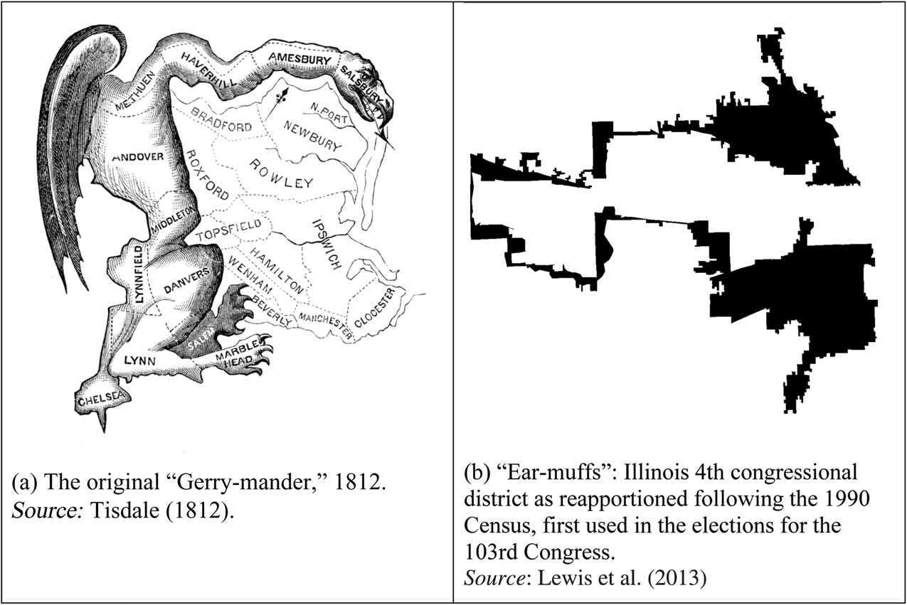
Figure 1. Examples of non-compact districts
We present the first longitudinal analysis of district compactness for all Canadian districts from 1867 to the present. For comparison, we perform the same analysis for US congressional districts. We find little variation in district compactness across time in Canada despite considerable change in the boundary-drawing procedures. In the United States, by contrast, districts became significantly less compact following the 1960s Supreme Court decisions that required equal representation by population and established the principle of creating minority-majority districts. Well-documented examples of partisan gerrymandering by state legislatures have no doubt exacerbated the trend toward non-compactness, as has the emergence of ever more sophisticated computer-aided geodemographic analysis tools (Levine, Reference Levine2021; Monmonier, Reference Monmonier2001).
Historical context
District compactness has received limited analytic attention in Canada. Historically, it is well documented that governing parties drew boundaries in ways that improved their electoral fortunes (Emery, Reference Emery2016). From Confederation to 1903, redistricting occurred by government bill; a majority government could therefore impose its preferences. Ward (Reference Ward1950: 27) documents these partisan machinations in detail, noting that “tampering was done with some hesitation and pretense of principle in 1872, with a gay abandon in 1882, and with dignity and persistence in 1893.” From 1903 until 1952, boundaries were determined by a parliamentary committee to which the governing party appointed a majority of members. In Courtney's (Reference Courtney2001: 20) estimation, the “great majority” of these processes “were partisan and blatantly self-serving affairs.”
The 1964 Electoral Boundaries Readjustment Act introduced a system whereby boundary schemes are determined by arm's-length commissions in each province. Each commission is chaired by a judge selected by the province's chief justice, and its other two members, generally academics and lawyers, are appointed by the Speaker of the House of Commons. The legislation sets out criteria to be considered by the commissioners. There is no requirement of absolute population equality among districts (and therefore voter parity) as in the United States. Rather, districts may vary in population by 25 per cent relative to the average district population within the province, and even greater deviation is possible “in extraordinary circumstances.” Deviation from representation by population can only be justified by consideration of the representation of “communities of interest” and “communities of identity,” as well as sustaining a “manageable geographic size.” The system has not been subject to extensive judicial review; however, the Supreme Court found in the 1991 Reference re Provincial Electoral Boundaries (Sask.), commonly refered to as the Carter decision, that section 3 of the Charter of Rights and Freedoms, which entrenches citizens’ right to vote, guarantees “effective representation” through the boundary-drawing process, thereby sanctioning deviation from voter equality in recognition of community interests, history, and minority representation.
Shifting boundary drawing from the legislative arena to the discretion of independent commissions is understood to have depoliticized the boundary-drawing process (Courtney, Reference Courtney2001), although Pal (Reference Pal2015) notes that the vagueness of the criteria set out in the legislation and Carter permit considerable discretion, and therefore variability, in their application by the commissions. Indeed, Pal argues that Canadians should be concerned by commission boundary schemes in which the principle of voter parity is subordinated to regional or group representation objectives.
If district non-compactness is a reliable indicator of partisan manipulation, we may expect Canadian electoral district boundaries to become more compact with the 1966 RO, the first with boundaries drawn by commission. Moreover, if the Carter decision gave licence for commissions to craft district boundary schemes that prioritize minority representation over other criteria, we may expect post-Carter districts to be less compact with the 1996 RO.
The only prior analysis of district compactness in Canada is by Bélanger and Eagles (Reference Bélanger and Eagles2001), who compared the 1987 and 1996 ROs using two measures of compactness calculated in relation to perimeter length and area. Examining only two time points, they could not identify longer-term trends. Nevertheless, they concluded that natural geographic features such as coastlines and rivers and the inclusion of sometimes distant islands in coastal FEDs are important determinants of district shape and may inhibit the creation of compact districts.
The procedures by which boundaries are drawn are very different in the United States. The procedure by which US House of Representatives electoral districts are drawn is defined in federal and state law. A national formula determines how many seats each state will have following the decennial census; however, it is up to state legislatures to draw the boundaries. The criteria used to draw them are sometimes embedded in state constitutions or statutes. By one count, 17 states require congressional districts to be compact, 11 states require consideration of communities of interest and 17 prohibit the drawing of boundaries for partisan advantage (Levitt, Reference Levitt2020). In most states, the majority party in the legislature has a free hand to draw congressional district boundaries and, in doing so, aid their co-partisans at the federal level. Partisan gerrymandering—that is, the intentional construction of districts that reliably elect members belonging to the governing party—has existed in the United States since the formation of parties (Engstrom, Reference Engstrom2013) and is as prevalent at the state level as it is at the federal level (Keena et al., Reference Keena, Latner, McGann McGann and Smith2021).
Prior to the landmark Supreme Court decisions Baker v. Carr (1962) and Wesberry v. Sanders (1964) characterized by Baker (Reference Baker1966) as the “reapportionment revolution,” states generally constructed districts out of county or municipal boundaries, resulting in substantial variation in the populations of districts. Afterward, districts within each state were required to have equal populations. The deliberate drawing of districts to ensure the legislative representation of minority groups is sanctioned by the 1965 Voting Rights Act. This is referred to as “affirmative racial gerrymandering,” as distinct from “negative racial gerrymandering,” the purpose of which is to demobilize African-Americans, Latinos and other minority groups. Numerous state legislative district schemes have been invalidated by the courts on this basis. Defining a legally defensible position between the “packing” and “cracking” of minority groups to eliminate discriminatory electoral practices has proven elusive, however, resulting in extensive legal challenge and judicial review. Between 1965 and 2013, the Voting Rights Act also required state boundary schemes to be “precleared” by the Department of Justice in designated states, putting a brake on negative racial gerrymanders. This was invalidated by the Supreme Court in Shelby County v. Holder in 2013, however. With the end of preclearance and the Supreme Court's 2019 decision in Rucho v. Common Cause that partisan gerrymandering was beyond the court's purview, many observers believe that partisan and negative racial gerrymandering will only intensify.
Taking a long historical perspective, we may expect that US congressional districts are likely to be relatively more compact prior to the 1960s than afterward, when voter parity was effectively constitutionalized and affirmative racial gerrymandering sanctioned. We may also expect compactness to decline as partisan gerrymandering has been facilitated by modern computer-aided techniques and fuelled by the intensification of partisan polarization. This expectation is supported by Ansolabehere and Palmer (Reference Ansolabehere and Palmer2016) in their panoptic geostatistical analysis of all congressional district boundary schemes since 1790. They find that the distribution of districts along three measures of compactness varies modestly from the early republic until the 1971 postcensal redistribution, after which it dramatically increases.
Data and methods
Political scientists and legal scholars have developed numerous indicators of district compactness. Barnes and Solomon (Reference Barnes and Solomon2021) identify 24 distinct measures (see also Niemi et al., Reference Niemi, Grofman, Carlucci and Hofeller1990). The most commonly referenced geometric measures quantify variation in relationship between district area and perimeter (the Polsby-Popper measure and related approaches), the ratio of a district's area to that of a minimum bounding circle (the Reock method) or convex hull, and the degree to which the shape is symmetrical. Kaufman et al. (Reference Kaufman, King and Komisarchik2021) find that these and other indicators correlate poorly with one another and that the degree of correlation depends on the sample of districts analyzed. This suggests that compactness is a multidimensional concept that is not easily captured by a singular measurement and that it cannot be reliably quantified by adding or multiplying other measures. Kaufman et al. (Reference Kaufman, King and Komisarchik2021) pursue a novel empirical approach to overcome this dilemma. Working from the premise that humans “know compactness when they see it,” they surveyed multiple populations—undergraduates, judges and legislators, and users of the Mechanical Turk platform—and asked them to rank selected images of US state legislative districts from most to least compact. They found a very high level of agreement among the respondents’ visual assessments. They then calculated multiple compactness measures for 17,896 congressional and state districts. Machine-learning techniques were then used to train a series of models that predicted the ranking the survey respondents would have given each district, which were then combined into an ensemble model. The result is an algorithm that, given digital boundaries as inputs, computes an index ranging from 1 (most compact) to 100 (least compact) for each district. The source code for this algorithm is publicly available as an R package (Kaufman, Reference Kaufman2021).
We used this code to calculate compactness scores and standard errors for every FED in each of the 18 Canadian federal ROs, from 1867 to the present, listed in Table 1. For comparison, we did the same for the 22 US congressional district schemes adopted after all but one decennial census since 1790.Footnote 2 Congressional district digital boundary files are retrieved from Lewis et al. (Reference Lewis, DeVine, Pritcher and Martis2013). We also coded each district based on whether it is adjacent to an ocean coast or Great Lake using national coastal waters boundary datasets (Office for Coastal Management, 2018; Statistics Canada, 2006a). This enables us to separately analyze districts whose boundaries are partially defined by an impassable water barrier and therefore not subject to the discretion of legislators or independent boundary commissions.
District compactness trends
To visualize district shapes at different levels of compactness, Figure 2 displays representative districts at the 2nd, 25th, 50th, 75th and 98th percentiles for both countries. The most extreme cases are excluded. (In Canada, these are the districts representing the Northwest Territories and Nunavut. In the United States, the least compact district is California's 5th district following the 1960 reapportionment, an anomalous case with three noncontiguous parts: the eastern part of the City of San Francisco, Treasure Island in the bay, and the Farallon Islands, which are 48 km to the west, in the Pacific Ocean.) The characteristics of the districts at these breakpoints are as expected. Those toward the compact end of the scale are rectilinear in appearance; those at the least compact end are complex and feature multiple disconnected parts. The districts at the 75th percentile both have protruding “arms”; those at the 25th are compact in appearance but have irregular or crenellated perimeters. We note that the compactness score at each percentile are six to nine points lower in Canada than in the United States, although we have no explanation for this.
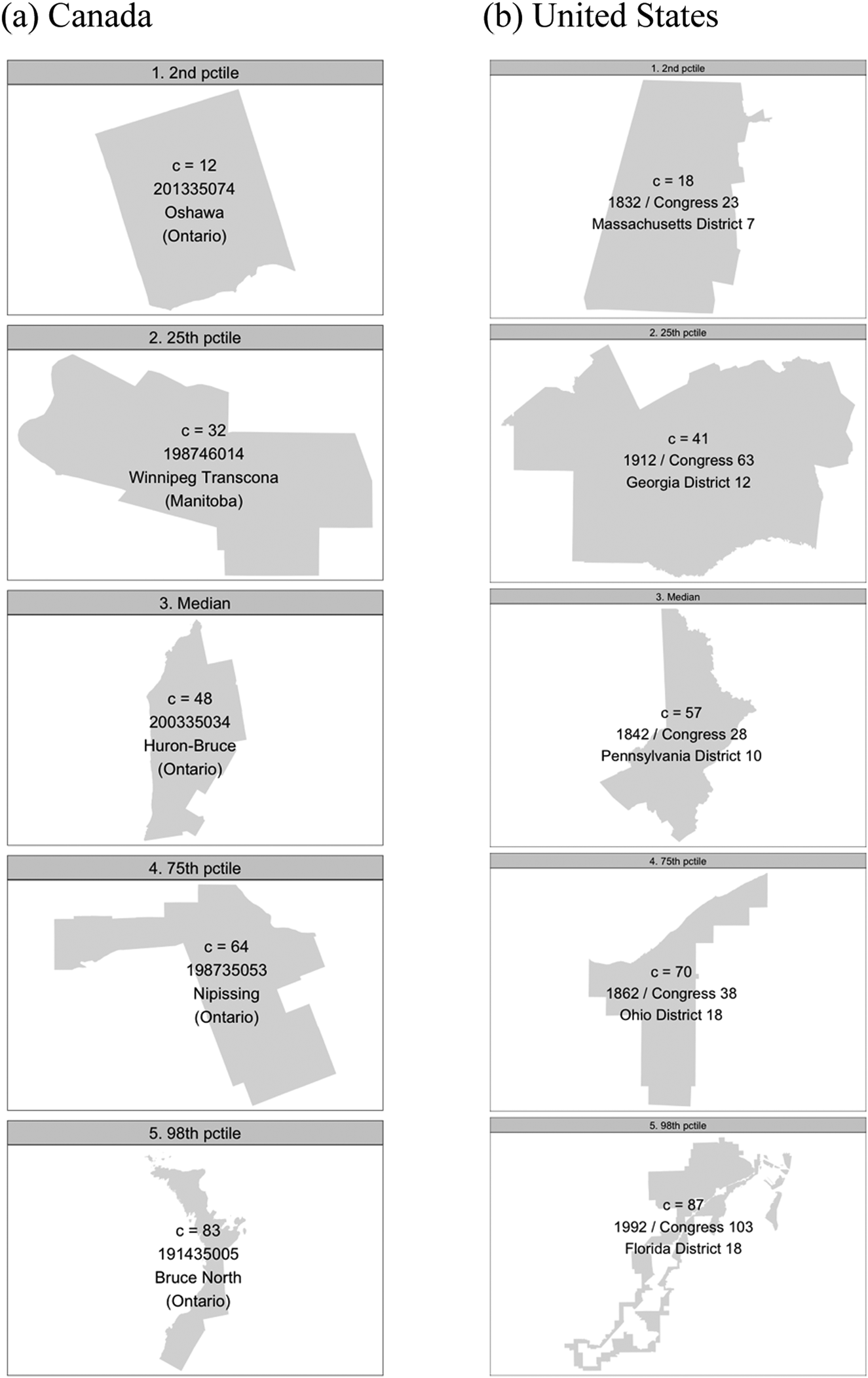
Figure 2. Canadian and American districts at different compactness percentiles
Figures 3 and 4 present a summary of the distribution of compactness scores for each postcensal boundary scheme across the entirety of post-Confederation Canadian and post-1789 US history. For each set of boundaries, the figure plots the overall distribution, the median compactness score (the vertical line in the centre of each distribution) and the 25th and 75th percentile scores (the vertical lines to the right and left of the median line in each distribution). It is striking that there is very little variation in Canada. The median and interquartile range values are virtually the same in ROs from 1867 to the 2013 RO, despite the expansion of national territory and European settlement over this period. There is little evidence that the 1964 Electoral Boundaries Readjustment Act or the 1991 Carter decision had any effect on the distribution of compactness scores.

Figure 3. Distribution of district compactness scores—Canada
Note: Lower values indicate greater compactness. Vertical lines indicate the 25th, 50th and 75th percentile. Year indicates proclamation of the new national representation order.

Figure 4. Distribution of district compactness scores—United States
Note: Lower values indicate greater compactness. Vertical lines indicate the 25th, 50th and 75th percentile. Year indicates first House of Representatives in which boundaries were used following the decennial census. No reapportionment occurred following the 1920 Census.
We see greater variation in the United States. The range of compactness varies in the early years of the republic but stabilizes between 1840 and 1950. This is unsurprising given that there was considerable continuity in district boundaries, which in many cases respected county boundaries. (Indeed, analysis of Lewis’ metadata indicates that one-third of all historic congressional districts are counties or aggregations of counties.) As Ansolabehere and Palmer (Reference Ansolabehere and Palmer2016) note, the shift from early variability to stability also reflects the western inland expansion of the United States. The median district became more compact from 1790 through 1830 as the proportion of districts whose boundaries are defined by the complex geographies of ocean coasts declined.
Bélanger and Eagles (Reference Bélanger and Eagles2001) and Ansolabehere and Palmer (Reference Ansolabehere and Palmer2016) both note that ocean and Great Lake coastlines can skew district compactness results. We therefore also examined the distributions of compactness scores and identified the districts at the same percentiles for noncoastal districts alone. We recognize that excluding districts that border oceans and Great Lakes is something of a blunt instrument—62 per cent of districts were coastal in 1867, declining to 43 per cent in 2013, so a large number of districts would be excluded (see Table 1). One might also exclude districts whose borders are partially coterminous with provincial or state boundaries, rivers and other water bodies; however, few districts would remain. Nevertheless, the results (not shown) are as expected—the distributions of compactness scores are lower overall, yet the general trends over time remain the same.
Discussion
Our exploration of FED compactness in Canada compared to the United States is illuminating in several respects. First, applying Kaufman et al.'s (2021) technique to the US districts supports Ansolabehere and Palmer's (Reference Ansolabehere and Palmer2016) earlier findings: that the 1960s were a major disruptor of long-established patterns. The Supreme Court decisions that required equal population, combined with federal enforcement of the Voting Rights Act, produced districts that were considerably less compact in pursuit of effective racial representation. At the same time, majority parties in state legislatures used increasingly sophisticated techniques to consolidate their electoral positions through partisan gerrymandering and, in some cases, frustrate affirmative racial gerrymandering through packing and cracking, while preserving voter parity.
It is striking, however, that no such pattern is visible in Canada despite equally important changes to boundary-drawing criteria and processes. As Ward (Reference Ward1950: 46) notes, the only real criterion applied in boundary drawing prior to the 1960s was to secure partisan advantage, a criterion governing parties maximally exploited. One would therefore have expected the introduction of independent boundary commissions and legislated criteria to have affected district compactness. Moreover, one would have expected boundary drawing in the wake of Carter to have produced more geometrically complex districts in pursuit of effective community representation. Our analysis indicates, however, that these changes had no effect on the overall distribution of district compactness scores.
This finding generates several potential lines of inquiry. It may be that district compactness is a meaningful indicator of gerrymandering (affirmative or negative) in the United States but not in Canada. We hypothesize that the strict voter parity requirement in the United States forces the construction of more irregularly shaped districts in pursuit of racial representation and partisan advantage. In contrast, the Canadian system's tolerance for significant population variation among districts enables boundary drawers to consider communities of interest and identity, and also “manageable geographic size,” without creating geometrically elaborate districts. This could be investigated by comparing specific redistricting processes and products in selected states and provinces in relation to social and electoral geography. In an analysis of the 2003 RO and 2001 Census, for example, Forest (Reference Forest2012), found that Canada's population inequalities among ridings systematically disadvantage visible minorities. Our datasets would enable similar analyses over a much longer period.
Another matter to consider is the very different average population size of districts in the two countries—109,444 in Canada versus 761,179 in the United States according to the most recent census figures. As Rodden (Reference Rodden2019) notes, US districts often have populations greater than those of midsize cities, resulting in the dilution of (often racialized, Democratic-leaning) urban interests within broader (often white, Republican-leaning) hinterlands. This is not the case in Canada. In tandem with permitted population variation, smaller districts may enable the drawing of boundaries that enable “effective representation” without necessitating the creation of districts with elaborate geometries.
Similar to the recent US analyses discussed, our brief investigation considered only the geometric features of districts. A useful extension would be to leverage census data at lower levels of geographic aggregation to investigate the distribution of populations within and across adjacent districts to assess the degree to which ethic, racial, linguistic, and other groups are, inadvertently or intentionally, cracked and packed.
Conclusion
In this article we have introduced new datasets and tools for the spatial and nonspatial analysis of all Canadian FEDs since 1867. These comprise a comprehensive set of district identification codes, a complete set of digital boundary files, a correspondence table linking our district identification codes to Sevi's (Reference Sevi2021) candidate dataset, and a set of historical census data aggregated to FEDs. We hope that they will unlock new research on Canadian political development and representation. All files are posted to the Borealis data repository at https://doi.org/10.5683/SP3/4E8DCR.
To illustrate their utility, we also presented an application using the digital boundary files: an investigation of the compactness of Canadian FEDs compared to US congressional districts. Our findings are perhaps surprising. Compared to their US counterparts, whose compactness changes in expected ways over time, Canadian FEDs show very little variation in the distribution of district compactness scores over the 18 ROs spanning 1867 to the present. We conclude by advancing several hypotheses for future investigation.
Acknowledgments
The authors are grateful to the following research assistants for their work on different aspects of this project: Moira Benedict, Tyler Girard, Amanda Miknev and Kandys Paterson.
Funding statement
This project was supported by SSHRC Insight Grant #435-2019-0224 and internal seed grants from the Faculty of Social Science, University of Western Ontario.
Data availability statement
Supplementary materials for this article are available at Taylor, Zachary; Lucas, Jack; Kirby, J. P.; Hewitt, Christopher Macdonald, 2023, “Replication Data for ‘Canada's Federal Electoral Districts, 1867–2021: New Digital Boundary Files and a Comparative Investigation of District Compactness.’ Canadian Journal of Political Science.” https://doi.org/10.5683/SP3/4E8DCR, Borealis.
Competing interests
To avoid a conflict of interest, the review process for this article was handled by Dr. David Peterson. The editors of the Canadian Journal of Political Science thank him for assisting us in this guest editor role.


 Open access