


1. Introduction
Solid particles immersed in aqueous electrolytes usually carry a net surface charge which is screened by a diffuse ionic layer on the electrolyte side of the interface. Relative motion between the solid and liquid can occur when an external electric field acts on these charges, giving rise to particle motion known as electrophoresis (Hunter Reference Hunter1993). For diffuse layers much thinner than the particle size, the electrophoretic velocity is given by the Helmholtz–Smoluchowski formula (Hunter Reference Hunter1993) as  $\boldsymbol {U}=(\varepsilon \zeta /\eta )\boldsymbol {E}$, where
  $\varepsilon$ is the medium permittivity and
  $\eta$ its viscosity,
  $\boldsymbol {E}$ the applied electric field and
  $\zeta$ the zeta potential (the electrical potential at the slip plane; Delgado et al. Reference Delgado, Gonzalez-Caballero, Hunter, Koopal and Lyklema2005). In the presence of an alternating current (AC) field with amplitude
  $\boldsymbol {E}_0$, electrophoresis manifests itself as an oscillatory motion of the particle at the same frequency as the field, with a displacement amplitude given by
  $(\varepsilon \zeta /\eta )\boldsymbol {E}_0/\omega$, where
  $\omega$ is the angular frequency of the electric field. Observations of the fluid flow around micron-scale solid dielectric particles in an AC field has revealed a previously unobserved fluid flow pattern. Here we report fluid patterns around
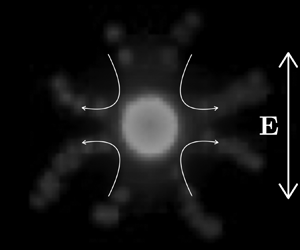
  $3\ \mathrm {\mu }\textrm {m}$ spheres exposed to low-frequency AC field imaged using fluorescent tracer particles (500 nm diameter). Figure 1 shows an example of these flow patterns. Significantly, the observed quadrupolar flow is not oscillatory. This paper presents a theoretical model that describes these observations by considering the effect of perturbations in the electrolyte concentration on the electro-osmotic flow around the particles. The gradients in electrolyte concentration occur due to particle surface conduction. The model for these phenomena predicts the previously reported stationary flows observed around dielectric micropillars (
 $20\ \mathrm {\mu }\textrm {m}$ diameter) subjected to AC fields (Calero et al. Reference Calero, Fernández-Mateo, Morgan, García-Sánchez and Ramos2021). The surface conduction of these micropillars is relatively small, and the model was based on the approximation for small Dukhin number (the ratio of surface to bulk conductance; Delgado et al. Reference Delgado, Gonzalez-Caballero, Hunter, Koopal and Lyklema2005). However, this is not small for particles with a typical size around
  $1\ \mathrm {\mu }\textrm {m}$ or smaller. As a first attempt to model stationary flows for arbitrary values of the Dukhin number, we develop a theoretical scheme for weak electric fields. Gamayunov, Murtsovkin & Dukhin (Reference Gamayunov, Murtsovkin and Dukhin1986) argued that stationary quadrupolar flows may appear around charged dielectric spheres as a consequence of concentration polarization and/or induced charge within the electrical double layer (EDL). The flow pattern due to EDL polarization in a DC field was analysed in detail by Dukhin & Murtsovkin (Reference Dukhin and Murtsovkin1986). Here we extend the analysis of Schnitzer & Yariv (Reference Schnitzer and Yariv2012) to the case of AC electric fields and describe the stationary flow around a charged colloidal sphere as a function of frequency, albeit with the restriction of a binary electrolyte with equal ionic diffusivities. The latter assumption is valid for our experiments with KCl aqueous solutions and greatly simplifies the theoretical treatment of the problem. In this work we focus on the simplest system, in which stationary flows for AC fields arise due to surface conduction, where there is already an asymmetry between counter-ions and co-ions. Experimental data on the stationary electro-osmotic flow around microparticles are in agreement with the predictions of the model. These flows could be important in controlling the interaction between microscopic particles subjected to low-frequency AC electric fields (around 1 kHz or less) and in general for any technique relying on AC fields for electrical manipulation of dielectric particles.

Figure 1. Experimental paths of 500 nm particles around a fluorescent latex sphere of  $3\ \mathrm {\mu }\textrm {m}$ diameter along with streamlines predicted by (2.32). The applied field magnitude and frequency are
  $80\ \textrm {kV}\ \textrm {m}^{-1}$ and 292 Hz.
2. Theory
Schnitzer & Yariv (Reference Schnitzer and Yariv2012) derived a mathematical model for the electrokinetic flows of symmetric electrolytes at large zeta potentials in the limit of thin EDL, including surface conduction effects. Building on this work, we modelled the stationary flows induced by AC fields around charged cylinders with small Dukhin number (Calero et al. Reference Calero, Fernández-Mateo, Morgan, García-Sánchez and Ramos2021). We now explore the case of finite Dukhin number and weak electric fields (Schnitzer et al. Reference Schnitzer, Zeyde, Yavneh and Yariv2013). To this end, we consider a negatively charged dielectric sphere immersed in a binary electrolyte and subjected to an AC electric field with amplitude  $E_0$ and angular frequency
  $\omega$. We assume that this frequency is low enough so that the EDL is in quasi-equilibrium (
 $\omega \ll \sigma /\varepsilon$, with
  $\varepsilon$ and
  $\sigma$ denoting the liquid permittivity and conductivity, respectively). We use a dimensionless formulation where length is scaled with the radius of the particle
  $a$, electric potential with the thermal voltage
  $\phi _{{ther}}=k_{B}T/ze$ (where
  $k_{B}$ is Boltzmann's constant,
  $T$ absolute temperature,
  $z$ ionic valence and
  $e$ elementary charge), time with
  $\eta /\varepsilon E_{{ther}}^{2}$ (where
  $E_{{ther}}=\phi _{{ther}}/a$ is the thermal electric field), pressure with
  $\varepsilon E_{{ther}}^{2}$, and ion concentrations with typical salt concentration
  $c_0$. Thus, diffusion constants are non-dimensionalized with
  $\varepsilon a^{2}E_{{ther}}^{2}/\eta$, velocities with
  $\varepsilon E_{{ther}}^{2}a/\eta$, and the typical Reynolds number is
  ${Re}=\rho _m \varepsilon E_{{ther}}^{2}a^{2}/\eta ^{2}$, with
  $\rho _m$ the liquid mass density. The surface charge on the dielectric is non-dimensionalized with
  $\varepsilon \phi _{{ther}}/\lambda _D$, where
  $\lambda _D$ is the Debye length.
The conservation equations for the concentration of positive  $(c_+)$ and negative
  $(c_-)$ ions are, respectively,
 \begin{gather} \boldsymbol{\nabla}\boldsymbol{\cdot}({-}c_+\boldsymbol{\nabla}\phi-\boldsymbol{\nabla} c_+)+\alpha_+\boldsymbol{u}\boldsymbol{\cdot}\boldsymbol{\nabla} c_+{+}\alpha_+\frac{\partial c_+}{\partial t}=0, \end{gather}
 \begin{gather}\boldsymbol{\nabla}\boldsymbol{\cdot}(c_-\boldsymbol{\nabla}\phi-\boldsymbol{\nabla} c_-)+ \alpha_-\boldsymbol{u}\boldsymbol{\cdot}\boldsymbol{\nabla} c_-{+}\alpha_-\frac{\partial c_-}{\partial t}=0, \end{gather}
where  $\alpha _{+}$ and
  $\alpha _{-}$ are the reciprocals of the non-dimensional diffusion constants
  $D_{+}$ and
  $D_{-}$ for positive and negative ions, respectively, and the liquid velocity is
  $\boldsymbol {u}$. In the bulk electrolyte outside the EDL, electro-neutrality (
 $c_+=c_-=c$) means that these equations can be combined to give
 \begin{gather} D\nabla^{2}c=\boldsymbol{u}\boldsymbol{\cdot}\boldsymbol{\nabla} c+\frac{\partial c}{\partial t}, \end{gather}
 \begin{gather}\boldsymbol{\nabla}\boldsymbol{\cdot}(c\boldsymbol{\nabla}\phi)=\gamma\left(\frac{\partial c}{ \partial t}+\boldsymbol{u}\boldsymbol{\cdot}\boldsymbol{\nabla} c\right), \end{gather}
where  $D=2/(\alpha _++\alpha _-)$ and
  $\gamma =(\alpha _+-\alpha _-)/2$. Equation (2.3) is the diffusion equation for the ion concentration. Equation (2.4) is essentially the equation for the electric potential, where
  $\gamma$ is a parameter that is related to the asymmetry in ion mobility.
The boundary conditions on the surface of the charged dielectric sphere are as follows (Schnitzer & Yariv Reference Schnitzer and Yariv2012). The normal flux of co-ions (anions in our case) is zero:
 \begin{equation} c\frac{\partial\phi}{\partial n}-\frac{\partial c}{\partial n}=0. \end{equation}
The normal flux of counter-ions (cations in our case) equals the surface divergence of EDL cation flux:
 \begin{equation} -c\frac{\partial \phi}{\partial n}-\frac{\partial c}{\partial n}=2\,{Du}\boldsymbol{\nabla}_s^{2}(\phi+\ln c), \end{equation}
where Du is a Dukhin number defined as  ${Du}=(1+2\alpha _+)|q_s|\lambda _D$, with
  $q_s$ denoting the non-dimensional intrinsic surface charge. Here the normal derivative is from the dielectric to the electrolyte. In the literature (Delgado et al. Reference Delgado, Gonzalez-Caballero, Hunter, Koopal and Lyklema2005), the Dukhin number is defined as
  ${Du_o}=K_s/(\sigma a)$, where
  $K_s$ is the surface conductance. For large negative zeta potential (the case in this work), the relation between these two definitions is
  ${Du_o}\approx {Du}\,2D_{+}/(D_{+}+D_{-})$. Here Du can be considered a fixed quantity if the surface charge is fixed. In this work we assume this to be the case, i.e. variations in salt concentration do not lead to variations in the intrinsic surface charge. Also, note that the boundary conditions (2.5) and (2.6) neglect the charging of the EDL at the particle surface, in contrast to the modelling of induced-charge electro-osmosis (ICEO) phenomena with AC fields (Squires & Bazant Reference Squires and Bazant2004). As shown in Schnitzer & Yariv (Reference Schnitzer and Yariv2014) for dielectric particles and moderate fields, the induced zeta potential associated with induced charges in the EDL is negligibly small compared with the thermal voltage.
The liquid velocity and pressure satisfy the Navier–Stokes equations for negligible Reynolds number:
 \begin{equation} 0={-}\boldsymbol{\nabla} p+\nabla^{2}\boldsymbol{u}+\nabla^{2}\phi\boldsymbol{\nabla}\phi, \quad \boldsymbol{\nabla}\boldsymbol{\cdot}\boldsymbol{u}=0, \end{equation}
where the Coulomb term is present because gradients in ion concentration can lead to induced charge in the bulk, through (2.4). In these equations we neglect the term  ${Re}\partial \boldsymbol {u}/\partial t$ because it is negligible for particles with radii of the order of microns and frequencies less than 100 kHz. In other words (using dimensional quantities), this is negligible when
  $\rho _m\omega a^{2}/\eta \ll 1$. Thus, (2.7a,b) are quasi-static in the sense that time is implicit. The boundary condition at the particle surface is
  $\boldsymbol {u}=\boldsymbol {U}+\boldsymbol {u}_s$, where
  $\boldsymbol {U}$ is the translational velocity of the particle centre and
  $\boldsymbol {u}_s$ is the slip velocity generated at the EDL (Prieve et al. Reference Prieve, Anderson, Ebel and Lowell1984):
 \begin{equation} \boldsymbol{u}_s=\zeta\boldsymbol{\nabla}_s\phi-4\ln\left(\cosh(\zeta/4)\right)\boldsymbol{\nabla}_s \ln c. \end{equation}
The zeta potential  $\zeta$ is related to the intrinsic charge by the following (Hunter Reference Hunter1993):
 \begin{equation} q_s=2\sqrt{c}\sinh(\zeta/2). \end{equation}
The translational velocity  $\boldsymbol {U}$ is determined by the condition that the total hydrodynamic stress equals zero at the surface of the sphere (Schnitzer et al. Reference Schnitzer, Zeyde, Yavneh and Yariv2013). Far from the particle, at infinity, the fluid velocity is zero. At this point, the reference frame can be changed to one that is attached to the particle. The quasi-static equations for velocity and pressure are the same, and the new boundary conditions are
  $\boldsymbol {u}=\boldsymbol {u}_s$ at the particle surface,
  $\boldsymbol {u}=-\boldsymbol {U}$ at infinity. Under an applied AC electric field, the sphere velocity
  $\boldsymbol {U}$ is an oscillating function of time, with zero time average (from symmetry).
Following Schnitzer et al. (Reference Schnitzer, Zeyde, Yavneh and Yariv2013), we now perform a power expansion of the amplitude of the applied AC electric field  $\beta \equiv E_0/E_{ther}$:
  $c=1+\beta c_1+\beta ^{2} c_2+\dots$,
  $\phi =\beta \phi _1+\beta ^{2}\phi _2 +\dots$,
  $\boldsymbol {u}=\beta \boldsymbol {u}_1+\beta ^{2} \boldsymbol {u}_2+\dots$,
  $p=\beta p_1+\beta ^{2} p_2+\dots$ The linear approximation provides a fluid velocity that is oscillatory in time, while the stationary electro-osmotic flow around the sphere is found at second order in
  $\beta$.
2.1. Linear response
Salt concentration and potential satisfy
 \begin{equation} D\nabla^{2} c_1=\frac{\partial c_1}{\partial t},\quad\nabla^{2}\phi_1=\gamma\frac{\partial c_1}{\partial t}, \end{equation}
with boundary conditions as follows: at  $r=1$,
 \begin{equation} \frac{\partial c_1}{\partial r}+{Du}\,\boldsymbol{\nabla}_s^{2}(\phi_1+c_1)=0, \quad \frac{\partial c_1}{\partial r}-\frac{\partial \phi_1}{\partial r}=0, \end{equation}
where  $\nabla _s^{2}$ is the surface Laplacian, and at
  $r\to \infty$,
 \begin{equation} c_1=0, \quad \phi_1={-}\cos(\omega t)r\cos\theta. \end{equation}
Assume that positive and negative ions have the same mobility, so that  $\gamma =0$. Since the applied field is an oscillating function in time with angular frequency
  $\omega$, we write
  $c_1$ and
  $\phi _1$ as
  $c_1=Re[\tilde {c}_1\textrm {e}^{\textrm {i}\omega t}]$,
  $\phi _1=Re[\tilde {\phi }_1\textrm {e}^{\textrm {i}\omega t}]$. The complex functions satisfy
 \begin{equation} D\nabla^{2}\tilde{c}_1=\textrm{i}\omega \tilde{c}_1, \quad\nabla^{2}\tilde{\phi}_1=0. \end{equation}
Given that both  $\tilde {c}_1$ and
  $\tilde {\phi }_1$ are of the form
  $f(r)\cos \theta$, the solutions are found as
 \begin{equation} \tilde{c}_1=C\textrm{e}^{{-}k(r-1)}\frac{1+kr}{r^{2}}\cos\theta,\quad \tilde{\phi}_1={-}r\cos\theta+F\frac{\cos\theta}{2r^{2}}, \end{equation}
where  $k=\sqrt {\textrm {i}\omega /D}$, and
 \begin{equation} C =\frac{3 \,{Du}}{2+2k+k^{2}+{Du}(k+2)^{2}},\quad F =\frac{2\,{Du}(1+k+k^{2})-(2+2k+k^{2})}{2+2k+k^{2}+{Du}(k+2)^{2}}. \end{equation}
 The limit of zero frequency ( $k=0$)
 \begin{equation} \tilde{c}_1=\frac{3\,{Du}}{2+4\,{Du}}\frac{\cos\theta}{r^{2}},\quad \tilde{\phi}_1={-}r\cos\theta+\frac{{Du}-1}{2+4\,{Du}}\frac{\cos\theta}{r^{2}} \end{equation}
is coincident with that given by Schnitzer & Yariv (Reference Schnitzer and Yariv2012), and by Hunter (Reference Hunter1993) for thin double layers and a highly charged surface. At infinite frequency ( $k\to \infty$),
 \begin{equation} \tilde{c}_1=0,\quad \tilde{\phi}_1={-}r\cos\theta+\frac{2\,{Du}-1}{2+2\,{Du}}\frac{\cos\theta}{r^{2}}. \end{equation}
Here it can be seen that  $F/2=(2\,{Du}-1)/(2\,{Du}+2)$ is the low-frequency value of the Maxwell–Wagner–O’Konski dipole coefficient (O'Konski Reference O'Konski1960). The frequency dependence of the dipole coefficient
  $F/2$ is coincident with that given in Shilov et al. (Reference Shilov, Delgado, Gonzalez-Caballero and Grosse2001) for a highly charged surface, with thin double layer and equal ion mobilities, because
  $\gamma =0$ is set in (2.10a,b).
The fluid flow is oscillatory in time and governed by the equations
 \begin{equation} \nabla^{2} \boldsymbol{u}_1=\boldsymbol{\nabla} p_1,\quad\boldsymbol{\nabla}\boldsymbol{\cdot}\boldsymbol{u}_1=0, \end{equation}
with slip velocity at  $r=1$ given by
 \begin{equation} \boldsymbol{u}_{s1}=\zeta_0\boldsymbol{\nabla}_s\phi_1-4\log\left(\cosh(\zeta_0/4)\right)\boldsymbol{\nabla}_s c_1. \end{equation}
At infinity the fluid velocity goes to  $\boldsymbol {u}_{1}\to -Re[U_1\textrm {e}^{\textrm {i}\omega t}]\hat {\boldsymbol {z}}$. Here
  $U_{1}$ is determined by the condition that the total hydrodynamic stress is zero on the sphere, which leads to
 \begin{equation} U_{1}=\zeta_0\frac{2+2k+k^{2}+2\,{Du}(1+k)}{2+2k+k^{2}+{Du}(k+2)^{2}} +8\log\left(\cosh(\zeta_0/4)\right)\frac{ {Du}(1+k)}{2+2k+k^{2}+{Du}(k+2)^{2}}. \end{equation}
The slip velocity is then  $\boldsymbol {u}_{s1}=\frac {3}{2}Re[U_1\textrm {e}^{\textrm {i}\omega t}]\sin \theta \hat {\theta }$. At the limit of zero frequency,
 \begin{equation} U_{1}=\frac{\zeta_0(1+{Du})+4\,{Du}\log\left(\cosh(\zeta_0/4)\right)}{1+2\,{Du}}; \end{equation}
taking into account that  $\zeta _0$ is negative, this agrees with the expression given by Schnitzer et al. (Reference Schnitzer, Zeyde, Yavneh and Yariv2013). The latter was shown to be equivalent to the expression provided by O'Brien (Reference O'Brien1983) for large absolute zeta potential.
2.2. Quadratic response
The equations for salt concentration and potential at second order in  $\beta$ are
 \begin{equation} D\nabla^{2} c_2=\frac{\partial c_2}{\partial t}+\boldsymbol{u}_1\boldsymbol{\cdot}\boldsymbol{\nabla} c_1,\quad\nabla^{2}\phi_2={-}\boldsymbol{\nabla}\phi_1\boldsymbol{\cdot}\boldsymbol{\nabla} c_1, \end{equation}
with boundary conditions at  $r=1$ given by
 \begin{equation} \frac{\partial c_2}{\partial r}+{Du}\,\boldsymbol{\nabla}_s^{2}(\phi_2+c_2)=\frac{{Du}}{2}\boldsymbol{\nabla}_s^{2}c_1^{2}, \quad \frac{\partial c_2}{\partial r}-\frac{\partial \phi_2}{\partial r}=c_1\frac{\partial \phi_1}{\partial r}, \end{equation}
while at  $r\to \infty$ both
  $c_2$ and
  $\phi _2$ go to zero.
The time-averaged velocity and pressure satisfy
 \begin{equation} \nabla^{2}\langle\boldsymbol{u}_2\rangle=\boldsymbol{\nabla} \langle p_2\rangle, \quad \boldsymbol{\nabla}\boldsymbol{\cdot}\langle\boldsymbol{u}_2\rangle=0. \end{equation}
Here the body force is zero since  $\nabla ^{2}\phi _1=0$. The boundary condition at
  $r=1$ is a time-averaged slip velocity,
 \begin{equation} \langle\boldsymbol{u}_{2s}\rangle =\zeta_0\boldsymbol{\nabla}_s\langle\phi_2\rangle+\langle\zeta_1\boldsymbol{\nabla}_s\phi_1\rangle -4\ln\left(\cosh\left(\frac{\zeta_0}{4}\right)\right)\boldsymbol{\nabla}_s\left\langle c_2-\frac{c_1^{2}}{2}\right\rangle\!-\!\tanh\left(\frac{\zeta_0}{4}\right)\langle\zeta_1\boldsymbol{\nabla}_s\phi_1\rangle, \end{equation}
with  $\zeta _1=-c_1\tanh (\zeta _0/2)$ from (2.9) and fixed
  $q_s$. From symmetry, at infinity
  $\boldsymbol {u}_2\to 0$. Therefore, the time-averaged velocity can be derived from the time averages
  $\langle c_2\rangle$ and
  $\langle \phi _2\rangle$. The equations for
  $\langle c_2\rangle$ and
  $\langle \phi _2\rangle$ are
 \begin{equation} \nabla^{2} \langle c_2\rangle =\frac{1}{2D}Re\left[\boldsymbol{\nabla} \tilde{c}_1\boldsymbol{\cdot} \tilde{\boldsymbol{u}}_1^{*}\right], \quad \nabla^{2}\langle\phi_2\rangle ={-}\frac{1}{2}Re\big[\boldsymbol{\nabla}\tilde{\phi}_1\boldsymbol{\cdot}\boldsymbol{\nabla} \tilde{c}_1^{*}\big], \end{equation}
where the time-averaged product of two oscillating functions satisfies  $\langle\, f(t)g(t)\rangle =\frac {1}{2}Re[fg^{*}]$. The boundary conditions at
  $r=1$ are now written as
 \begin{equation} \left.\begin{gathered} \frac{\partial \langle c_2\rangle}{\partial r} +{Du}\,\boldsymbol{\nabla}_s^{2}\langle\phi_2+c_2\rangle = \frac{{Du}}{4}\boldsymbol{\nabla}_s^{2}|\tilde{c}_1|^{2}, \\ \frac{\partial \langle c_2\rangle}{\partial r} -\frac{\partial \langle \phi_2\rangle}{\partial r} = \frac{1}{2}Re\left[\tilde{c}_1\frac{\partial \tilde{\phi}_1}{\partial r}\right]. \end{gathered}\right\} \end{equation}
The source terms in the equations (2.26a,b) and the independent terms in the boundary conditions (2.27) are linear combinations of  $P_0(\cos \theta )$ and
  $P_2(\cos \theta )$, where
  $P_n(x)$ is the Legendre polynomial of degree
  $n$. Therefore,
  $\langle c_2\rangle$ and
  $\langle \phi _2\rangle$ can be written as
  $\langle c_2\rangle =c_{20}(r)+c_{22}(r)P_2(\cos \theta )$ and
  $\langle \phi _2\rangle =\phi _{20}(r)+\phi _{22}(r)P_2(\cos \theta )$. Only the terms proportional to
  $P_2(\cos \theta )$ are important for the slip velocity (2.25). The general solutions of (2.26a,b) for these terms that decay at infinity are of the form
 \begin{equation} c_{22} =\frac{A}{r^{3}}+Re[G_c(r)],\quad \phi_{22} =\frac{B}{r^{3}}+Re[G_\phi(r)], \end{equation}
where  $A$ and
  $B$ are constants that are determined from the boundary conditions, and
  $G_c$ and
  $G_\phi$ are particular solutions of the equations
 \begin{equation} \left.\begin{gathered} \frac{1}{x^{2}}\frac{\partial}{\partial x}\left(x^{2}\frac{\partial G_c}{\partial x}\right)- \frac{6G_c}{x^{2}} =\frac{CU_1^{*}k\textrm{e}^{k}}{2D}\textrm{e}^{{-}x}g_c(x),\\ \frac{1}{x^{2}}\frac{\partial}{\partial x}\left(x^{2}\frac{\partial G_\phi}{\partial x}\right)- \frac{6G_\phi}{x^{2}}={-}\frac{Ck\textrm{e}^{k}}{2}\textrm{e}^{{-}x}g_\phi(x), \end{gathered}\right\} \end{equation}
where  $x=kr$, and
 \begin{equation} \left.\begin{gathered} g_c(x) =2x^{{-}3}+2x^{{-}2}+\tfrac{2}{3}x^{{-}1}-k^{3}(x^{{-}6}+x^{{-}5}+\tfrac{2}{3}x^{{-}4}),\\ g_\phi(x)=2x^{{-}3}+2x^{{-}2}+\tfrac{2}{3}x^{{-}1}+k^{3}F^{*}(x^{{-}6}+x^{{-}5}+\tfrac{2}{3}x^{{-}4}). \end{gathered}\right\} \end{equation}
Note that the operator  $D_r^{2}\equiv ({1}/{r^{2}})\,{\textrm {d}}/{\textrm {d}r}(r^{2}({\textrm {d}}/{\textrm {d}r}))-{6}/{r^{2}}$ comes from the Laplacian operator in spherical coordinates when using solutions of the form
  $f(r)P_2(\cos \theta )$. The right-hand sides in (2.29) are linear combinations of terms like
  $x^{m}\textrm {e}^{-x}$. A solution of the equation
  $D^{2}_x G =x^{m} \textrm {e}^{-x}$ that decays at infinity is
 \begin{equation} G(m,x)=\tfrac{1}{5}(\varGamma(m+5,x)x^{{-}3}-\varGamma(m,x)x^{2}), \end{equation}
where  $\varGamma (m,x)$ is the incomplete Gamma function. Therefore, we construct
  $G_c$ and
  $G_\phi$ as linear combinations of
  $G(m,x)$ with
  $m=-6,-5,\dots ,-1$, and from here we obtain
  $c_{22}$ and
  $\phi _{22}$.
Finally, the time-averaged slip velocity (2.25) is obtained as  $\langle \boldsymbol {u}_{2s}\rangle =U\sin (2\theta )\hat {\theta }$, where
  $U$ is given in Appendix A. With this slip velocity on the sphere, the time-averaged velocity field is as follows (Gamayunov et al. Reference Gamayunov, Murtsovkin and Dukhin1986; Squires & Bazant Reference Squires and Bazant2004):
 \begin{equation} \langle\boldsymbol{u}_{2}\rangle=U\left(\frac{(1-r^{2})(1+3\cos 2\theta)}{2 r^{4}}\hat{r}+\frac{\sin 2\theta}{r^{4}}\hat{\theta}\right). \end{equation}
The streamlines of this velocity field are shown in figure 2(a).

Figure 2. (a) Streamlines of the field represented by (2.32). (b) Slip velocity  $U$ as a function of
  $\omega /D$. Here
  $\zeta =-4$,
  $D=4.5$.
Figure 2(b) shows  $U$ as a function of
  $\omega /D$ (
 $\omega {a}^{2}/D$ with dimensions) for different values of the Dukhin number. While the theory for small Dukhin number leads to a velocity that scales linearly with Du, the current model predicts a saturation. For example, figure 2(b) shows that the slip velocities for
  $Du=0.1$ and
  $Du=1$ differ by around 10 %. It is clear that the intensity of the flow around the particle decreases beyond the characteristic dimensional frequency
  $\omega _c=D/a^{2}$, which is the reciprocal of the ion diffusion time for the radius
  $a$. For frequencies much greater than this,
  $U$ decays as
  $\omega ^{-1/2}$, and this frequency-dependent behaviour stems from the diffusion equation for the salt (2.13a,b). The mechanism that produces the quadratic flow is a consequence of the polarization of ion concentration, which decreases as
  $\omega ^{-1/2}$.
3. Experiments
The flows around single particles were imaged using a simple microfluidic channel. This consists of a straight polydimethylsiloxane (PDMS) channel 1 cm long with inlet and outlet reservoirs, fabricated using standard soft lithography. The channel cross-section is  $50\ \mathrm {\mu }\textrm {m} \times 50\ \mathrm {\mu }\textrm {m}$. The inlet and outlet reservoirs are sealed with metal cylinders that serve as the electrodes for the electric field. Fluorescent (500 nm and
  $3\ \mathrm {\mu }\textrm {m}$) carboxylate particles were suspended in an aqueous solution of potassium chloride (KCl) with a conductivity of
  $\sigma =1.7\ \textrm {mS}\ \textrm {m}^{-1}$. The
  $3\ \mathrm {\mu }\textrm {m}$ particle concentration was very low (no more than three or four particles in the channel at any one time). In order to prevent particles from sticking to the channel walls, these were pretreated with a solution of 0.1 % (w/v) Pluronic F-127 in deionized water (a non-ionic surfactant that adsorbs onto the PDMS) for at least 30 min. The peak-to-peak amplitude of the AC applied voltages was 1600 V over the frequency range from 100 Hz to 5 kHz. Below 100 Hz, the
  $3\ \mathrm {\mu }\textrm {m}$ particle oscillations due to the combination of electro-osmosis and zero-order electrophoresis are too large in amplitude to allow accurate measurement of the steady flows around the particles. For frequencies above 5 kHz, the magnitude of the quadrupolar flow is too weak compared to the Brownian motion of the tracer particles.
The trajectories of the 500 nm tracers were imaged using fluorescent microscopy. These tracers describe a three-dimensional flow pattern around the  $3 \ \mathrm {\mu }\mathrm {m}$ particles. The microscope objective was focused at approximately a horizontal plane at the centre of the large particle. Out of all the tracer trajectories, only those that were approximately within the focal plane were used (as shown in figure 1).
The  $3\ \mathrm {\mu }\textrm {m}$ particles oscillate due to electrophoresis, but also have a small drift due to small pressure fluctuations within the microchannel. Thus, in order to measure the fluid velocity around these particles with respect to them, a MATLAB program was developed to track the position of single
  $3\ \mathrm {\mu }\textrm {m}$ particles and to place this large particle in the centre of a reference frame. This process is described in the supplementary movie available at https://doi.org/10.1017/jfm.2021.650. The videos of fluid flow thus have the large particle at a fixed position in the centre of the image, with the smaller tracer particles flowing around it. Particle tracking velocimetry of the tracers provides a set of velocities at given positions in the plane that are then compared with the theoretical flow field (2.32) through a least-squares fitting analysis with a single fitting parameter,
  $U$, the maximum slip velocity. Finally, the slip velocity and the experimental error are estimated from the average and dispersion of the values determined from analysis of each streamline.
Figure 3 shows experimental data on the slip velocity as a function of frequency, along with the predictions of the model. Typical parameters for carboxylated latex beads are  $\zeta =-75$ mV and
  $K_s=1$ nS (Ermolina & Morgan Reference Ermolina and Morgan2005). The figure shows that for the expected Dukhin number (
 $Du=0.392$), the theoretical prediction overestimates the velocity by a factor of between 2 and 3.

Figure 3. Experimental slip velocity  $U$ versus frequency of the applied field (
 $E_0=80\ \textrm {kV}\ \textrm {m}^{-1}$,
  $\sigma =1.7\ \textrm {mS}\ \textrm {m}^{-1}$,
  $a=1.5\ \mathrm {\mu }\textrm {m}$ and zeta potential is set to
  $\zeta _0=-75$ mV). Theoretical curves are shown for different values of Du:
  ${Du_o}=K_s/(\sigma a)$ with
  $K_s=1$ nS (——);
  ${Du}=(1+2\alpha _+)|q_s|\lambda _D$ (- - - -);
  ${Du_o}=K_s/(\sigma a)$ with
  $K_s=0.12$ nS as obtained by a least-squares fitting (
 $\cdots \cdots$).
4. Discussion and conclusions
This paper describes observations of stationary flows around dielectric spheres. Quadrupolar fluid flows driven by electro-osmosis have been predicted around metal spheres (Squires & Bazant Reference Squires and Bazant2004). However, in this case the slip velocity has a different origin, namely, ICEO. In the case of a charged dielectric sphere, the rectified fluid flow arises from the polarization of electrolyte concentration (concentration-polarization electro-osmosis, CPEO) that results from the surface conductance around the sphere. As shown in Calero et al. (Reference Calero, Fernández-Mateo, Morgan, García-Sánchez and Ramos2021), the induced charge on a dielectric sphere leads to an associated induced zeta potential that is much smaller than the variation in zeta potential due to concentration polarization. This implies that CPEO velocities are much higher than ICEO velocities for the case of dielectric surfaces.
Our mathematical model predicts quadrupolar flows with a velocity magnitude that vanishes for frequencies higher than  $\omega _c=D/a^{2}$, in agreement with experimental observations. A quantitative comparison between theory and experiment shows that the velocity magnitude is overestimated by the present model for typical values of Du measured for latex spheres. The nonlinear model assumes weak electric fields (
 $E_0a < k_{B}T/e$), but in the experiments
  $E_0a\approx 120\ \mathrm {mV}\approx 5 k_{B}T/e$. However, for AC fields the characteristic scale of the ion diffusion equation is the smaller of
  $a$ or the diffusion penetration depth
  $\sqrt {D/\omega }$. This suggests that the condition of weak fields could be relaxed for high frequencies and rewritten as
  $E_0\ell < k_{B}T/e$, with
  $\ell$ the smaller of the two scales. For example, for
  $f\approx 3$ kHz, the characteristic length is
  $\ell \sim a/5$ and
  $E_0\ell \sim k_{{B}}T/e$.
The effects of this flow pattern on the pair interactions between particles have been theoretically studied in the context of induced-charge electrophoresis and compared to that of dielectrophoresis (DEP) (Saintillan Reference Saintillan2008). Interestingly, the induced motion between particles decays for large distances as  $(a/r)^{2}$ due to the hydrodynamic interaction, and as
  $(a/r)^{4}$ due to the DEP interaction (with
  $r$ the distance between particle centres). Clearly, the hydrodynamic interaction is more important than the DEP interaction when the particles are separated by distances of several diameters. From our experiments and theory for CPEO around dielectric spheres, we expect hydrodynamic interactions between particles to decrease with ionic strength and vanish for frequencies much greater than
  $D/a^{2}$. Curiously, these trends have been found by Mittal et al. (Reference Mittal, Lele, Kaler and Furst2008) in experiments with latex microparticles subjected to AC fields, although they attributed this behaviour to the interaction between induced dipoles on the particles.
Supplementary movie
Supplementary movie is available at https://doi.org/10.1017/jfm.2021.650.
Funding
P.G.-S. and A.R. acknowledge financial support from the European Regional Development Fund and the Spanish State Research Agency (MCI) under contract PGC2018-099217-B-I00.
Declaration of interests
The authors report no conflict of interest.
Data availability statement
The data that support the findings of this study are openly available in the University of Southampton repository at https://doi.org/10.52.58/SOTON/D1898.
Appendix A. Expression for U
In this appendix we provide the expression for the maximum stationary slip velocity on the sphere,  $U$ (see (2.32)). We have checked that
  $U$ coincides with the expression of Schnitzer et al. (Reference Schnitzer, Zeyde, Yavneh and Yariv2013) for
  $k=0$. It is given by
 \begin{align} U &={-}\frac 32\zeta_0Re\left[B_1+B_2+G_\phi(k)\right] -\frac 14\tanh\left(\zeta_0/2\right)Re \left[(1+k)C(1-F^{*}/2)\right] \nonumber\\ &\quad +6\log\left(\cosh(\zeta_0/4)\right)Re\left[A_1+A_2+G_c(k)\right] \nonumber\\ &\quad -\left(4\log\left(\cosh\left(\frac{\zeta_0}{4}\right)\right)+\tanh\left(\frac{\zeta_0}{4}\right) \tanh\left(\frac{\zeta_0}{2}\right)\right)\frac{|C(1+k)|^{2}}{4}, \end{align}
where
 \begin{gather} \left.\begin{gathered} A_1 ={-}2\,{Du}\frac{3G_\phi(k)+kG_\phi'(k)}{3+12\,{Du}} +\frac 23{Du}\frac{(1+k)(1+F^{*})C}{3+12\,{Du}}+{Du} \frac{|C(1+k)|^{2}}{3+12\,{Du}},\\ B_1 =A_1+\frac{3kG_\phi'(k)-(1+k)(1+F^{*})C}{9}, \end{gathered}\right\} \end{gather}
 \begin{gather} A_2 =\frac{(1+2\,{Du})kG_c'(k)-6\,{Du}G_c(k)}{3+12\,{Du}}, \quad B_2 =\frac{-2\,{Du}kG_c'(k)-6\,{Du}G_c(k)}{3+12\,{Du}}, \end{gather}
 \begin{align} G_c(x)&=\frac{CU_1^{*}k\textrm{e}^{k}}{2D}[2G({-}1,x)/3+2G({-}2,x)+2G({-}3,x)\nonumber\\ &\quad -k^{3}(2G({-}4,x)/3+G({-}5,x)+G({-}6,x))], \end{align}
 \begin{align} G_\phi(x)&={-}\frac{Ck\textrm{e}^{k}}{2}[2G({-}1,x)/3+2G({-}2,x)+2G({-}3,x)\nonumber\\ &\quad +k^{3}F^{*}(2G({-}4,x)/3+G({-}5,x)+G({-}6,x))]. \end{align}


 Open access