


Following the publication of popular books such as Wheat Belly (Davis, Reference Davis2011) and Grain Brain (Perlmutter, Reference Perlmutter2013), consumer interest in gluten-free products grew. In 2009, about 1,200 new products made gluten-free claims; by 2016, more than 6,100 new product introductions made the claim (Economic Research Service [ERS], 2018a). The zealousness of gluten-free advocates reached such a zenith that parodies, such as “How to Become Gluten Intolerant,” emerged (Sears, Reference Sears2018). Eventually, regulators got involved. The Food and Drug Administration (FDA) reached a final ruling in 2013 regarding the requirements for “gluten-free” labels.Footnote 1
Many requests and suggestions were made to the FDA during the creation of gluten-free labeling standards. A noteworthy request urged the FDA to require a declaration of the presence of gluten on the Nutrition Facts label. Ultimately, the request was deemed outside the scope of the final labeling requirements ruling. Because the purpose of Nutrition Facts labels is to guide consumers in healthy food selections consistent with dietary recommendations (FDA, 2018; Van den Wijngaart, Reference Van den Wijngaart2002), the denial of the aforementioned request suggests gluten-free food products are not any healthier than products containing gluten. However, results from a survey conducted by the Mintel Group Ltd. (2016) indicate that 73% of consumers believe gluten-free products to be healthier than their gluten-containing counterparts. Similarly, Navarro (Reference Navarro2016) found that consumers perceive food products to be healthier if a gluten-free label is present. This common perception is the leading argument individuals without celiac disease provide for adhering to a gluten-free diet (Mintel Group Ltd., 2016).
Recent consumer surveys indicate that a gluten-free diet has become one of the most popular health food trends in the United States (Miller, Reference Miller2016).Footnote 2 Interestingly, the prevalence of celiac disease in U.S. citizens remained stable at around 1% of the population, yet in 2014 an estimated 5.4 million people without gluten intolerance adhered to a gluten-free diet (Choung et al., Reference Choung, Unalp-Arida, Ruhl, Branter, Everhart and Murray2017).Footnote 3 For these reasons, the recent interest in purchasing gluten-free food products is being described as a fad (Reilly, Reference Reilly2016). The gluten-free market is valued at US$6.6 billion (Aziz, Hadjivassiliou, and Sanders, Reference Aziz, Hadjivassiliou and Sanders2015; Talley and Walker, Reference Talley and Walker2016).
Despite the rising interest in gluten-free foods, there is scant evidence on the impact of this trend on consumer food demand or on farmer welfare. The main objective of this article is to fill this void in the literature.
Historically, U.S. wheat producers and millers relied on the increasing demand for wheat flour to justify further investments. However, per capita flour use began to decrease in 2000 as low-carbohydrate diets were introduced (e.g., Atkins, Reference Atkins2002; ERS, 2018b). In 2000, per capita wheat flour use was estimated at 146.3 pounds/person and ultimately reached the record low of 132.5 pounds/person in 2011 before rebounding somewhat in more recent years (ERS, 2018b). Acres planted for wheat production fell by 25% from 1997 to 2010, and would have decreased by nearly 35% since 1997 to the 2017–2018 projection of 46 million acres (ERS, 2018c; NASS, 2018). The reduction in wheat acreage decreased the U.S. share of global wheat exports from an average of 25% during 2001–2005 to 15% in 2017 (ERS, 2018c). While a variety of factors have likely contributed to wheat’s demise, the gluten-free diet is one potential culprit.Footnote 4
Wheat is typically sold at the retail level in the form of flour, and is used as a byproduct in many cereal and bakery products (ERS, 2018d). For this reason, we focus on aggregate demand for U.S. cereal and bakery food products. We estimate an Inverse Almost Ideal Demand System (IAIDS) using personal consumption expenditure (PCE) and price index data reported by the Bureau of Economic Analysis (BEA, 2018) along with LexisNexis data collected using the search term “gluten free.” Welfare effects are determined by constructing an equilibrium displacement model that links the supply of disaggregated farm commodities to consumer food demands at the retail level. This model relies on the flexibility and demand shock estimates derived from IAIDS estimates.
1. Data
1.1. Expenditure and price data
The BEA defines consumer spending, or PCEs, as the goods and services purchased by, or on the behalf of, U.S. residents (BEA, 2018). Although annual and quarterly estimates are available, we make use of monthly estimates. It is important to note that monthly PCE values reported on the BEA website are annualized. In other words, the reported PCE for any given month reflects the amount by which it would have changed over a year’s time if it had continued to grow at the given rate. For instance, the PCE value reported for March 2017 represents the 2017 PCE value if PCE continued to grow at the same rate that it grew in March. Hence, monthly PCE values reported by the BEA are equivalent to monthly consumer spending multiplied by 12. As a result, we divide (annualized) monthly PCE estimates provided in BEA table 2.4.5U (BEA, 2007) by 12 to recover monthly expenditures for the food products discussed below from January 2004 to July 2018.
The BEA provides U.S. food expenditure information at aggregated and disaggregated levels. This allows total food expenditures to be calculated by summing the aforementioned monthly expenditures of various food groups: (1) cereal and bakery foods,Footnote 5 (2) meat, (3) dairy products, (4) eggs, (5) fruits and vegetables, (6) food away from home, (7) alcoholic beverages, (8) nonalcoholic beverages, and (9) “other” foods.Footnote 6 By dividing each of the food group expenditures by total food expenditures, we calculate the food group expenditure shares. This is done for all nine food products (categories). Following Okrent and Alston (Reference Okrent and Alston2011), we divide product expenditures by associated price indexes reported by the BEA (BEA, 2017a) to construct implicit quantity indexes. The annual mean expenditure shares can be found in Table 1. Price and quantity indexes are provided in Tables A1 and A2 in Appendix A.
Table 1. Average annual food expenditure shares

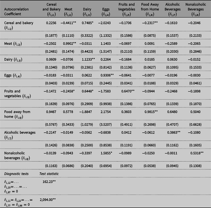
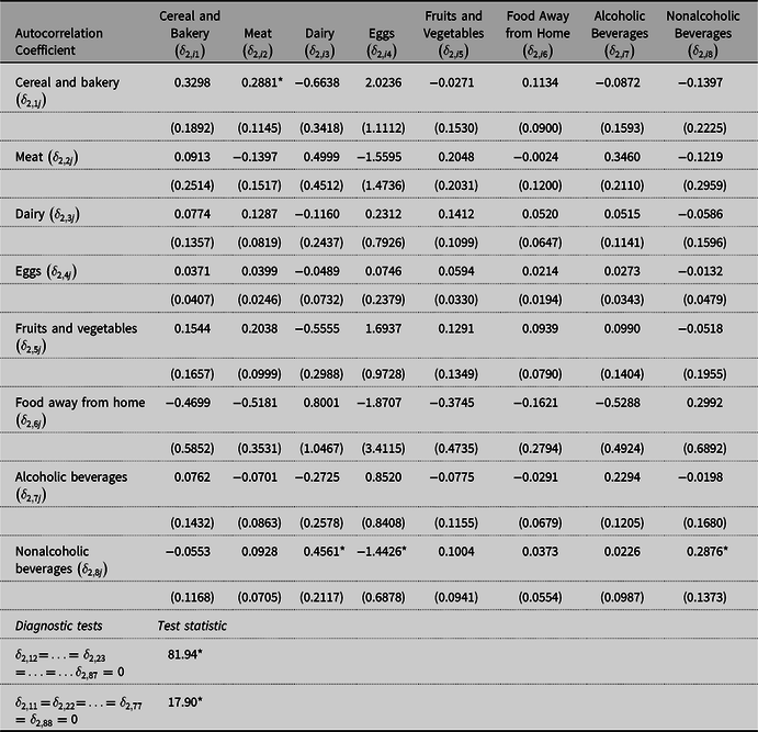
Table 2. Iterative seemingly unrelated regressions (ITSUR) estimates of the Inverse Almost Ideal Demand System (IAIDS) model using monthly LexisNexis data

* Statistical significance at the 5% level.
** Statistical significance at the 1% level.
Note: Standard errors are in parentheses.
1.2. Gluten-free index
Significant literature analyzing demand shifters exists, primarily in analyses of meat demand (Tonsor and Olynk, Reference Tonsor and Olynk2011). Examples of demand shifters include effects of health- and diet related-information (Adhikari et al., Reference Adhikari, Paudel, Houston, Paudel and Bukenya2006; Brown and Schrader, Reference Brown and Schrader1990; Chang and Kinnucan, Reference Chang and Kinnucan1991; Kinnucan et al., Reference Kinnucan, Xiao, Hsia and Jackson1997; Rickertsen, Kristofersson, and Lothe, Reference Rickertsen, Kristofersson and Lothe2003), food safety and product recall news (Burton and Young, Reference Burton and Young1996; Marsh, Schroeder, and Mintert, Reference Marsh, Schroeder and Mintert2004; Piggott and Marsh, Reference Piggott and Marsh2004), and advertising expenditures (Brester and Schroeder, Reference Brester and Schroeder1995; Kinnucan et al., Reference Kinnucan, Xiao, Hsia and Jackson1997; Park and Capps, Reference Park and Capps2002; Piggott et al., Reference Piggott, Chalfant, Alston and Griffith1996; Rickertsen, Reference Rickertsen1998).
As indicated by Just (Reference Just2001), it is not uncommon for media indexes to be used as demand shifters. In fact, Brown and Schrader (Reference Brown and Schrader1990), Chang and Kinnucan (Reference Chang and Kinnucan1991), Burton and Young (Reference Burton and Young1996), Kinnucan et al. (Reference Kinnucan, Xiao, Hsia and Jackson1997), Rickertsen, Kristofersson, and Lothe (Reference Rickertsen, Kristofersson and Lothe2003), Marsh, Schroeder, and Mintert (Reference Marsh, Schroeder and Mintert2004), and Piggott and Marsh (Reference Piggott and Marsh2004) search articles printed in popular newspapers and/or journals for specific verbiage to create media indexes to use as shifters of food demand. Using the LexisNexis database (academic version), we follow these studies and search the top 50 English Language newspapers in circulation from January 2004 to July 2018 for articles containing the verbiage “gluten free.”
Unlike Kinnucan et al. (Reference Kinnucan, Xiao, Hsia and Jackson1997), our index does not represent “net-publicity” by differentiating between positive and negative information. This distinction is made for a few reasons. The first, and most obvious, is that all gluten-free is anti-gluten. If this approach was adopted, indexes would be negative for all months and inaccurately portray changing interest in gluten-free over time. Moreover, discrimination between positive and negative information as portrayed by the media can be highly subjective (Liu, Huang, and Brown, Reference Liu, Huang and Brown1998; Mazzocchi, Reference Mazzocchi2006; Smith, van Ravenswaay, and Thompson, Reference Smith, van Ravenswaay and Thompson1988; Verbeke and Ward, Reference Verbeke and Ward2001). For these reasons, the gluten-free index is defined as the number of articles meeting aforementioned requirements in a given month.
Data were collected on a monthly basis, yielding 175 observations. A graph of gluten-free indexes from January 2004 to July 2018 is shown in Figure 1. LexisNexis data show steady, rising media coverage of gluten-free until mid-2014, after which coverage continues increasing, albeit at a decreasing rate.
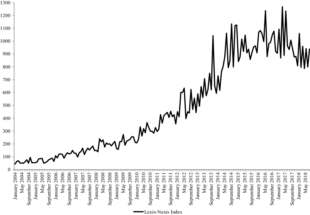
Figure 1. Monthly gluten-free index, 2004 to 2018.
2. Demand estimation
We first seek to determine the effect of the interest in gluten-free on food demand in the United States—specifically of food products inherently containing gluten. To do so, we estimate the changes in cereals and bakery food expenditure shares, as well as eight other foods.
The implementation of an inverse system of demands, where prices are a function of quantities, provides an alternative and fully dual approach to ordinary demand system(s) (e.g., Almost Ideal Demand System, AIDS). Inverse demands suggest food quantities are exogenous (supply is inelastic), and price must adjust to establish a market equilibrium. Specifying prices as a function of quantities is motivated by the perishability of many foods now consumed and, consequently, limited storage, by the biological lag inherent in the production of most food products and byproducts sold in the retail setting (Piggott and Marsh, Reference Piggott, Marsh, Lusk, Roosen and Shrogen2010). Because of the biological lag, many food products are essentially fixed in quantity in the short run (Christensen and Manser, Reference Christensen and Manser1977; Huang, Reference Huang1988) and the application of an inverse demand systems approach is warranted (Brown, Le, and Seale, Reference Brown, Lee and Seale1995; Chambers and McConnell, Reference Chambers and McConnell1983; Holt and Goodwin, Reference Holt and Goodwin1997; Huang, Reference Huang1988).
The IAIDS proposed by Eales and Unnevehr (Reference Eales and Unnevehr1994) is defined as
 $${w_{it}} = {\alpha _i} + \mathop \sum \limits_{j = 1}^n {\gamma _{ij}}\ln {x_{jt}} + {\beta _i}\ln Q + \mathop \sum \limits_{l = 0}^L {\theta _{il}}GF{I_{lt}} + {\rho _i}Trend{\rm{,}}$$
where
 $$\ln Q = {\alpha _0} + \mathop \sum \limits_{j = 1}^n {\alpha _j}\ln {x_{jt}} + {1 \over 2}\mathop \sum \limits_{i = 1}^n \mathop \sum \limits_{j = 1}^n {\gamma _{ij}}\ln {x_{it}}\ln {x_{jt}},$$
and  $${w_{it}}$$ represents the expenditure share of food i in month t
  $\left( {{w_{it}} = {{{p_{it}}{x_{it}}} \over M}} \right)$,
  $$M$$ represents total food expenditures, i = 1,…,9 representing cereal and bakery products, meat, dairy, eggs, fruits and vegetables, food away from home, alcoholic beverages, nonalcoholic beverages, and other foods, respectively, t = 1,…,175,
  ${x_{it}}$ represents quantity of food i demanded in month t,
  $$GF{I_t}$$ represents the number of articles printed in the top 50 English language newspapers in the United States in time t containing the verbiage “gluten free” lagged l months,
  $$Trend$$ is a time trend, and parameters to be estimated are
  ${\alpha _0},{\alpha _i},{\gamma _{ij}},$
 $${\beta _i}$$ (Eales and Unnevehr, Reference Eales and Unnevehr1994),
  ${\theta _i},$ and
  ${\rho _i}$.
The specification includes an index of interest in gluten-free food (via LexisNexis), much like the inclusion of a BSE consumer awareness indicator variable by Burton and Young (Reference Burton and Young1996). To ensure this index is indeed measuring (and representing) the popularity and effect of interest in gluten-free on food demand, rather than just an overall trend, a time trend is also included.Footnote 7
The nine demand equations represented by equation (1) are estimated as a system. One equation is dropped in the estimation to avoid singularity (we drop the “other” food category). The parameters of the omitted equation are recovered using Engel aggregation (adding up) restrictions. Typical demand restrictions of homogeneity, symmetry, and aggregation are imposed and treated as maintained hypotheses.Footnote 8 Often, the  $${\alpha _0}$$ parameter is difficult to estimate and may cause convergence issues, leading to difficulties in identifying parameter values. To alleviate such issues, this parameter is set to zero. The models are estimated using iterative seemingly unrelated regressions (ITSUR).
2.1. Estimation strategy
The empirical analysis is completed in several steps. First, models are estimated without an index in order to obtain starting values. Because of the nonlinearity of the system, it is possible for models to converge at different local optimums. The use of these starting values for various estimations, discussed subsequently, ensures that all models converge at the same local optimum.
Starting values are used to estimate equation (1) with the gluten-free index. The possibility of lagged effects is considered by sequentially including lag lengths and calculating necessary test statistics. Because of the dynamic nature of the model and the possibility of autocorrelation, Wald tests are used.Footnote 9 Because lagged values of the index are warranted, this suggests information obtained through media has an effect for the number of lagged months on food consumption. Consequently, the possibility of autocorrelation is a concern.Footnote 10
With time series data, the errors in equation (1) may not be serially independent, instead following a vector autoregressive scheme of order k. Moschini and Moro (Reference Moschini and Moro1994) note several options for estimating the structural parameters in equation (1) along with autocorrelation terms. Similarly to Holt and Goodwin (Reference Holt and Goodwin1997) and Piggott et al. (Reference Piggott, Chalfant, Alston and Griffith1996), we follow Anderson and Blundell (Reference Anderson and Blundell1982, Reference Anderson and Blundell1983) by estimating less restrictive  $\left( {n - 1} \right) \times \left( {n - 1} \right)$ autocorrelation matrix(es) of the general dynamic model:
 $${\varepsilon _{it}} = \mathop \sum \limits_j^{n - 1} {\delta _{k,ij}}{\varepsilon _{i,t - k}} + {v_{it}},$$
Where  $t = 1, \ldots ,175, 1 \lt k \lt 174 $, and
  $${v_{it}}$$ are independently, identically distributed normal random errors. Hence, it is not necessary to estimate an
  $nxn$ matrix of autocorrelation coefficients, but rather a
  $\left( {n - 1} \right) \times \left( {n - 1} \right)$ matrix of autocorrelation coefficients.Footnote 11
Including the necessary lags for each index, we obtain the residuals for  $n - 1$ share equations using the model specified in equation (1). Residuals are lagged K months and models are re-estimated using equation (3) as an error term in equation (1). To test whether each individual equation has autocorrelation, the following hypotheses are conducted:
 $${{\rm{H}}_1}:\;{\delta _{k,ij}} = 0,\forall i = j\,{\rm{versus }} \ {{\rm{H}}_{{\rm{1A}}}}:\;{\delta _{k,ij}} \ne 0,\forall i = j.$$
Further, to ensure that the less restrictive autocorrelation matrix is necessary, we test that (1) the autocorrelation coefficients are statistically different from each other and zero and (2) the off-diagonal elements in the autocorrelation matrix are statistically different from each other and zero:
 $${{\rm{H}}_2}:\;{\delta _{k,11}} = {\delta _{k,22}} = \ldots = {\delta _{k,88}} = 0\,{\rm{versus}} \ {{\rm{H}}_{{\rm{2A}}}}: {\rm{at \ least \ one}}\,{\delta _{k,ij}}\left( {\forall i = j} \right) \ne 0 $$
 $${{\rm{H}}_3}:\;{\delta _{k,12}} = {\delta _{k,23}} = \ldots {\delta _{k,78}} = 0\,{\rm{versus}} \ {{\rm{H}}_{{\rm{3A}}}}: {\rm{at \ least \ one}}\,{\delta _{k,ij}}\left( {\forall i \ne j} \right) \ne 0.$$
 The order of the error term autoregressive scheme is represented by the level of k − 1 for which we fail to reject  $${{\rm{H}}_2}$$.
2.2. Flexibility estimates
Using parameter estimates from equation (1) containing the error term from equation (3), gluten-free flexibilities are estimated as:
 $$f_i^{{\rm{GF}}} = \mathop \sum \limits_l^L \left( {{{{\theta _{il}}} \over {{{\bar w}_i}}}} \right)\overline {GF{I_l}} $$
where  $$f_i^{{\rm{GF}}}$$ represents the gluten-free flexibility of food i,
  $${\theta _{il}}$$ is a parameter estimated in the ith share equation,
  $\overline {GF{L_l}} $ represents the mean gluten-free index when lag length l is considered, and
  $${\bar w_i}$$ represents the mean expenditure share for food i.
Following Eales and Unnevehr (Reference Eales and Unnevehr1994), we estimate own- and cross-price flexibilities in the following way:
 $${f_{ij}} = - {\delta _{ij}} + {{{\gamma _{ij}} + {\beta _i}\left( {{w_j} - {\beta _j}\ln Q} \right)} \over {{{\overline w}_i}}},$$
where  $${f_{ij}}$$ represents own- or cross-price flexibilities,
  $${\delta _{ij}}$$ is the Kronecker delta,
  $${\gamma _{ij}}$$ and
  $$\beta $$s are model parameters, and
  $${\bar w_i}$$ represents the mean expenditure share for food i.
We follow Eales and Unnevehr (Reference Eales and Unnevehr1994) by describing own- and cross-price flexibilities as the percentage change in the price of the ith good when the quantity demanded increases by 1%. Demand for a commodity is flexible if a 1% increase in consumption leads to a more than 1% decrease in the marginal value of that commodity in consumption, and inflexible if an increase in consumption leads to a less than 1% decrease. Furthermore, goods are termed gross quantity substitutes if their cross-price flexibility is negative, and gross quantity complements if it is positive (Eales and Unnevehr, Reference Eales and Unnevehr1994; Hicks, Reference Hicks1956).
3. Equilibrium displacement model
To determine welfare effects, a partial equilibrium model of the agricultural sector is constructed. Alston (Reference Alston1991) and Wohlgenant (Reference Wohlgenant, Lusk, Roosen and Shogren2011) have discussed these models in detail. Okrent and Alston (Reference Okrent and Alston2012) provided a useful contribution surrounding equilibrium displacement models by linking demand estimates to supply using input–output tables. This article uses the basic framework in Lusk (Reference Lusk2017), who built on the Okrent and Alston (Reference Okrent and Alston2012) framework.
The model used here is the same as in Lusk (Reference Lusk2017) except we use the demand flexibilities and demand shocks resulting from the estimates outlined in the previous section. Full details of the model are provided in Lusk (Reference Lusk2017) and Okrent and Alston (Reference Okrent and Alston2012), so they are not repeated here; the key differences in the model used here versus their models are fully described in Appendix B.
4. Results
Optimal gluten-free index lag length specifications can be found in Table 2 along with parameter estimates from iterative seemingly unrelated regressions. Results suggest the gluten-free index has an effect for 3 months (L = 3) on food demand. Furthermore, test statistics associated with  $${{\rm{H}}_2}$$ indicate the error term is associated with an autoregressive order scheme of 2 (periods). Autocorrelation matrix coefficients (
 ${\delta _{k,ij}}$) are shown in Tables A3 and A4 in Appendix A. Uncompensated and compensated own-and cross-price flexibilities are shown in Tables 3 and B1, respectively, and gluten-free index flexibilities and scale flexibilities in Table 4.
Table 3. Uncompensated own- and cross-price flexibilities using iterative seemingly unrelated regressions (ITSUR) estimates of the Inverse Almost Ideal Demand System (IAIDS) model with monthly data

* Statistical significance at the 5% level.
** Statistical significance at the 1% level.
Note: Standard errors are in parentheses.
Table 4. Gluten-free media and scale flexibilities using iterative seemingly unrelated regressions (ITSUR) estimates of the Inverse Almost Ideal Demand System (IAIDS) model

* Statistical significance at the 5% level.
** Statistical significance at the 1% level.
Note: Standard errors are in parentheses.
Joint autocorrelation tests indicate share equations require separate (nonequal) autocorrelation coefficients  $$\left( {{{\rm{H}}_2}} \right)$$. A joint test of the off-diagonal elements in autocorrelation matrixes
  $$\left( {{{\rm{H}}_3}} \right)$$ further verifies the appropriateness of following Anderson and Blundell (Reference Anderson and Blundell1982, Reference Anderson and Blundell1983). Although autocorrelation is not present in each share equation, adding-up restrictions prohibit the deletion of an autocorrelation corrective term. Hence, if we fail to reject
  $${{\rm{H}}_1}$$ for the ith share equation, the autocorrelation coefficient is not statistically different from zero and
  $${\varepsilon _{it}} = {v_{it}}$$. When
  $${{\rm{H}}_1}$$ is rejected, the autocorrelation is corrected with the
  ${\delta _{k,ij}}\left( {i = j} \right)$ estimate.
Coefficients associated with the gluten-free index allow us to determine the effect of interest in gluten-free foods on demand for food—specifically cereal and bakery food products. When estimating cereal and bakery demand, the current period (L = 0) is statistically insignificant while all lagged values of the index are significant at the 1% level. The time trend coefficient is also significant at the 1% level. This ensures the index is measuring gluten-free interest while indicating the necessity of the time trend. The same results are observed for nonalcoholic beverages as for cereal and bakery products, and similar results are observed for dairy, eggs, and fruits and vegetables. Obverse results are associated with meat, food away from home, and alcoholic beverages, compared to cereal and bakery products. Only lagged values of the index are statistically significant for these food products, and they are associated with positive coefficients and statistically significant time trend coefficients.
It is interesting to note the lack of statistical significance for the current period (L = 0) gluten-free index across each share equation in the system of equations, and the associated statistical significance of the time trend. Given the necessity of lagged indexes and statistically significant changes in all food product expenditures over time, it appears the culmination of the popularity and/or media coverage of gluten-free over multiple months would help explain changes in food expenditures. In other words, an increase in gluten-free interest does not have immediate effects on food demand. If the relationship between indexes and expenditures is not invariant to lag length (i.e., positive relationship when L = 0, but negative when L = 1), the full relationship between each index and food expenditure cannot be determined by coefficient signs alone, and is ambiguous. Because of this, and the reliance on adding-up restrictions to recover coefficients associated with “other” foods, gluten-free flexibility estimates will provide more detailed effects of gluten-free interest on food expenditures.
4.1. Own- and cross-price flexibilities
Table 3 contains uncompensated own- and cross-price flexibility estimates. All own-price flexibility estimates are statistically different from zero. The own-price flexibilities of cereal and bakery food products, meat, fruits and vegetables, food away from home, alcoholic beverages, nonalcoholic beverages, and “other” foods indicate that these food products are inflexible goods. The cereal and bakery own-price flexibility measurement is not surprising given the wide array of substitutes captured by cross-price flexibilities: meat, eggs, food away from home, alcoholic beverages, and other foods.
Dairy, fruits and vegetables, and nonalcoholic beverages are considered gross quantity complements of cereal and bakery products. Results are consistent with findings from Okrent and Alston (Reference Okrent and Alston2011). Differences in results pertain to the relationship between cereal and bakery goods with alcoholic beverages; they report alcoholic beverages as a complement to cereal and bakery products.
4.2. Gluten-free flexibilities
The gluten-free flexibility measurement is of primary interest. Because (the majority) cereal and bakery foods inherently contain gluten, and nearly 5.4 million Americans have recently adopted the gluten-free lifestyle, it is logical to hypothesize that expenditures of such products would significantly decrease as interest in gluten-free foods increases. Although this is a large number of individuals, this faction represents ~1.7% of the total U.S. population. As a result, we expect gluten-free flexibility estimates to be small.
As shown in Table 4, the cereal and bakery gluten-free flexibility estimate (−0.0384) is statistically significant at the 1% level. Ceteris paribus, this means a 1% increase in the gluten-free index is associated with a 0.0384% decrease in cereal and bakery prices. Thus, the rise in popularity of gluten-free diets has significantly decreased the expenditures of products inherently containing gluten. However, significant effects are not limited to gluten-containing foods. Demand for dairy, eggs, fruits and vegetables, nonalcoholic beverages, and other foods decreases significantly (1% level) as interest in gluten-free increases. Conversely, a positive relationship between gluten-free interest and food away from home and alcoholic beverages is observed at the 1% significance level. In short, the estimated flexibilities range from −0.133 for eggs to 0.053 for meat, and all are significant at the 1% level.
Perhaps effects captured by model coefficients and estimated flexibilities should not be a surprise given results recently published in the literature. Take, for example, the lean finely textured beef (LFTB)—otherwise known as pink slime—fiasco in 2012. The media paid extra attention to LFTB, and Yadavalli and Jones (Reference Yadavalli and Jones2014) hypothesized that the media portrayal of LFTB would negatively affect the consumption of aggregate meat and beef cuts. However, their parameter estimates indicate that increased media attention did not immediately lead to significant changes in consumer demand across meats or within the beef category. Pork expenditures did not significantly decrease until 2 weeks after news reports of LFTB surfaced, but demand rose the following week. On the fourth week, no significant media effects were observed. Demand for turkey increased 2 weeks after news of LFTB broke, but significant effects on demand disappeared in the third week. Similar results were observed with Prime beef demand. Significant demand effects were not observed until week three, which was followed by decreased demand in week four. In short, Yadavalli and Jones (Reference Yadavalli and Jones2014) found effects of LFTB media coverage on meat demand to be delayed and short-lived. The use of monthly data in this study prohibits the determination of weekly or daily effects of gluten-free interest on food demand. However, results from Yadavalli and Jones (Reference Yadavalli and Jones2014) provide merit to the possibility of delayed media effects on food demand.
Robert Atkins published a book in Reference Atkins1972 advocating a low-carbohydrate diet he used to treat patients in the 1960s (see Atkins, Reference Atkins1972). Around the time it was rewritten in 2002 (see Atkins, Reference Atkins2002), the “Atkins diet” became increasingly popular. Similarly to this study, Tonsor, Mintert, and Schroeder (Reference Tonsor, Mintert and Schroeder2010) created a media index centered on the Atkins diet,Footnote 12 amongst other factors, to determine changes in meat demand. Because they focus on media information impacts on meat demand, effects on various meat products (e.g., beef, pork, and poultry) are evaluated. Results from their study indicate a positive relationship between net positive information associated with the Atkins diet (a high-protein, low-carbohydrate diet) and the demand for beef.Footnote 13 While separate meat categories are not considered in this study, we also find positive, significant effects of increased gluten-free interest on meat demand. It can be argued that the obsession with a gluten-free diet, especially for those who do not have celiac disease or gluten intolerance (i.e., 5.4 million Americans), is the present-day equivalent to the previous obsession with the Atkins diet. After all, the two diets represent the same guidelines (decreased carbohydrate consumption).
4.3. Welfare effects
The equilibrium displacement model calculates effects of changes relative to an initial equilibrium. This means we analyze effects of changes in retail demand for food products attributed to increased interest in gluten-free. Two scenarios are considered. The first scenario contains a partial impact of gluten-free interest where only a shock to cereal and bakery demand is considered, and the second scenario contains the full impact (of gluten-free interest) where all estimated demands are shocked.
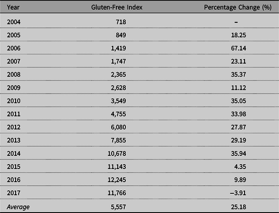
Because of the biological lag associated with the production of commodities and the subsequent consumption of final retail food products, we evaluate changes in annual producer welfare. By summing the number of articles containing the phrase “gluten-free” each year, we estimate average annual changes in the gluten-free index to be 25% (see Table A5 in Appendix A). For this reason, we use flexibility estimates presented in Table 4 to reflect changes in producer and consumer welfare for a 25% increase in newspaper articles rather than a 1% increase.
Producer surplus/deficit is equal to economic profits/losses, ignoring fixed costs, which do not vary with the volume of production. It should be noted that producer welfare changes are accrued to all producers of the commodity in question and the suppliers of inputs to producers (Just, Hueth, and Schmitz, Reference Just, Hueth and Schmitz2005). However, further delineating the incidence of these effects for the farming supply chain would require expanding the model to include the supply and demand of each input (Lusk, Reference Lusk2017). As a result, producer welfare estimates are presented with the understanding that changes are aggregated to capture upstream firms in addition to farmers.
Compensating variation is used to express changes in consumer welfare. This represents the amount of money that would need to be given to consumers to make them as well off as they were before the demand shock. It includes any extra expenditures consumers make following the demand shock and an estimate of the loss that occurs from consumers choosing a less desirable bundle of products. Although it would be nice to focus on compensating variation for specific products, only an aggregate change in compensating variation can be calculated across all goods because we have multiple demand curves (Wohlgenant, Reference Wohlgenant, Lusk, Roosen and Shogren2011). Because of this, we sum estimated changes in compensating for variation across goods.
4.3.1. Scenario 1: Partial impact
While Table 5 shows changes in producer surplus for all commodities included in this study, we primarily focus on changes in wheat and barley producer profits in this scenario because only cereal and bakery shocks are considered. Results indicate wheat and barley producer profits decrease by US$6.77 million/year and US$455,000 million/year, respectively, from increased interest in gluten-free. In addition, flexibility estimates indicate meat is a substitute for cereal and bakery foods. Ultimately, this translates to increases in profits for cattle, hog, and poultry producers.
Table 5. Partial impact effects of gluten-free interest on commodity prices and producer welfare from a shock to cereal and bakery retail demand

Abbreviations: PS, producer surplus.
An increase of US$562 million in consumer welfare is observed when summing estimated changes in compensating variation across all goods. Combining changes in consumer and producer surplus attributed to decreased demand for cereal and bakery products when newspaper articles on gluten-free increase by 25% suggests a net benefit in social welfare of US$1.5 billion. These results are presented in Table 6.
Table 6. Partial impact effects of gluten-free interest on retail prices, quantity, and consumer welfare from a shock to cereal and bakery retail demand

Abbreviations: CV, compensating variation; SW, social welfare.
We are not naïve to the fact that changes in demand for cereal and bakery foods at the retail level will also affect the consumption of other goods. After all, estimated cross-price flexibilities indicate that many foods are considered substitutes, for example, meat. As shown through results of implementing a partial impact, changes in retail food demand for all products will likely impact producer profits. However, producers must decide which crops to produce well in advance of planting and it may take years for producers to transition practices and produce alternative commodities because of crop-specific growing seasons. This poses an interesting conundrum surrounding the production practices and welfare of various commodity producers that can only be answered by considering the full impact of increased interest in gluten-free.
4.3.2. Scenario 2: Full impact
As indicated through own- and cross-price flexibility estimates, changes in quantity consumed affect the prices of other goods available for purchase. In other words, changes in preferences for particular goods affect the demand for their substitutes and complements. Scenario 2 investigates changes in producer and consumer welfare attributed to effects of rising interest in gluten-free on retail demand for all foods.
Changes in producer welfare are presented in Table 7. In this scenario, wheat and barley producers have not experienced decreases in profits as a result of increased interest in gluten-free foods. Instead, results suggest wheat and barley producer profits have increased by US$12.25 million per year and US$2.2 million/year, respectively. Given the negative relationship between retail demand for gluten-based food products and the media index, these results seem counterintuitive at first glance. However, results indicate that the outward shifts in meat and food away from home demand attributed to increases in gluten-free articles (more than) compensate for the inward shift in cereal and bakery demand. In what follows, we trace the flow of these competing demand shifts through the model.
Table 7. Full impact effects of gluten-free interest on commodity prices and producer welfare from a shock to all food demand

Input–output tables (produced by Okrent and Alston, Reference Okrent and Alston2012) show that 38% of the total cost of grain production was allocated to cereal and bakery products, 1.3% to fruits and vegetables, and 38% to other foods. Not only are these foods associated with negative flexibilities, but model results also indicate that the portion of wheat and barley allocated to food production decreased (0.0034%). Instead, a larger percentage (0.034%) was used in animal feed. In other words, the costs of grain production were being allocated differently—to animal production.
From 2004 to 2017, the supply of livestock increased, and producers of these products experienced increases in profits (most likely from increases in retail meat demand). Moreover, 16% of the cost of cattle production, 19% of other livestock, 14% of poultry and egg, and 23% of dairy farming production are attributed to food away from home. Interestingly, food away from home is associated with a positive flexibility, and about 17% of the remaining aforementioned cost of grain production is attributed to food away from home.
In short, this information suggests that the percentage of wheat that was once used to produce cereal and bakery products has decreased and is now being redistributed and used as feed in animal production. This results in a final product: meat. The extent to which grain production costs have changed is difficult to quantify; however, results suggest a portion of grain production costs are now indirectly allocated to meat, eggs, and dairy retail products through animal production—which was not the case beforehand—and a larger portion of these costs is allocated to alcoholic beverages. This also implies that a larger portion of aforementioned cattle, other livestock, poultry and egg, and dairy farming production costs have been allocated to food away from home. These changes have occurred to satisfy the decreased demands for cereal and bakery products and increased demand for meat and food away from home substitutes. Thus, it appears as though the decreased demand for cereal and bakery products at the retail level and increased demand for meat, food away from home, and alcoholic beverages have benefitted not only consumers, but also wheat, barley, cattle, pork, dairy, poultry, and egg producers.
As suggested by flexibility estimates, meat producers receive the largest increases in profit (US$3.7 billion/year). Specifically, cattle producers have received the largest increase, US$1.97 billion/year, and poultry producers the smallest increase, US$809 million/year. Only vegetable and melon, fruit and tree nut, and soybean producers have been negatively impacted by increased interest in gluten-free. Vegetable and melon producers have experienced the greatest profit losses, upward of US$112 million/year. In total, producer surplus is estimated to be US$5.67 billion/year.
Table 8 shows the sum of compensating variation across all nine retail food products. Estimates indicate that consumers experience a benefit of US$3 billion/year when the number of articles on gluten-free increases by 25%. Combining changes in consumer and producer welfare results in social economic welfare change. As indicated in Table 8, social welfare increases by US$8.8 billion/year—assuming the number of gluten-free-related newspaper articles increases by 25% each year.
Table 8. Full impact effects of gluten-free interest on retail prices, quantity, and consumer welfare from a shock to all food demand

Abbreviations: CV, compensating variation; SW, social welfare.
5. Conclusions
There has been much discussion and hype regarding gluten-free foods in recent years. Results suggest expenditures for cereal and bakery products decreased as the popularity of the gluten-free topic increased. The delayed effects of interest in gluten-free (as captured by IAIDS coefficients) are similar to findings by Yadavalli and Jones (Reference Yadavalli and Jones2014). Moreover, the effect of increased gluten-free interest is observed in expenditures for other food products not inherently containing gluten as well as respective changes in producer surplus. To satisfy changing consumer preferences, the use of wheat and barley supplied by producers is redistributed away from food production into animal production. These and other market-equilibrating adjustments result in minimal retail food price changes.
Flexibility estimates suggesting increases in expenditures for food products not inherently containing gluten yet bearing the label due to the labeling laws is not surprising considering annual retail snack and meat gluten-free sales totaled approximately US$4.4 billion and US$2.5 billion alone in 2016 (Mintel Group Ltd., 2016).Footnote 14 That is, two food categories not inherently containing gluten, yet bearing the gluten-free label, accounted for over half of the gluten-free-food sales at the retail level in 2016. In turn, these effects are transferred to producers. Thus, in addition to observing significant decreases in average food product expenditures that inherently contain gluten, such as cereal and bakery foods, we have also observed significant changes in food expenditures for products not inherently containing gluten, such as meat, and the profits producers receive.
Gluten-free flexibility estimates indicate that meat producers have benefited from the popularity of gluten-free and the labeling requirements. Our estimates suggest meat producer welfare has increased by US$3.7 billion/year. As outlined in the discussion under Scenario 2, a smaller portion of wheat and barley supply is (directly) allocated to food production and a larger portion to animal/livestock production to satisfy increases in meat demand. Consequently, any negative impacts wheat and barley producers would have incurred are outweighed by benefits attributed to shocks on other foods, such as meat, resulting in increased wheat and barley producer profits of US$14.5 million/year.
Although the construction of the media index used in this study aligns with those used in previous studies, future studies might benefit from disaggregated, filtered media indexes. For instance, including product-specific indexes (e.g., search terms “gluten free” and “meat”) along with an index that mentions no specific food categories might provide greater insight. However, this task is difficult when the “other” food category is included.
In short, the results presented in this study suggest expenditures on goods inherently containing gluten decreases as the popularity of gluten-free increases. This results in the redistribution of wheat and barley to aid in the production of substitutes for cereal and bakery food products, such as meat and food away from home. Whatever negative impacts have befallen wheat producers in recent years, this research suggests, somewhat unexpectedly, that rising interest in gluten-free food is not a major contributor, and may in fact have benefitted producers.
Appendix A
Table A1. Average annual price index
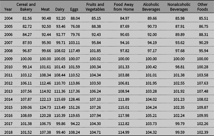
Table A2. Average annual quantity index

Table A3. Autocorrelation matrix of the Inverse Almost Ideal Demand System (IAIDS) model using monthly LexisNexis data (k = 1)
Note: Standard errors are in parentheses.
Table A4. Autocorrelation matrix of the Inverse Almost Ideal Demand System (IAIDS) model using monthly LexisNexis data (k = 2)
Note: Standard errors are in parentheses.
Table A5. Annual gluten-free index and percentage change: 2004–2017
Appendix B
B1. Equilibrium displacement model
The equilibrium displacement model used in this study is exactly the same as in Lusk (Reference Lusk2017), with four exceptions: (1) the demand side of the model is rewritten as quantity-dependent and the flexibilities shown in Table 3 are used to parameterize demands; (2) shocks to the model are given by the gluten-free flexibilities shown in Table 4 multiplied by the assumed percentage change in articles about gluten; (3) the expenditure and value of production data used to calculate welfare estimates are updated, and (4) a slight modification is made to the consumer welfare calculation to ensure consistency with our demand estimates.
Wohlgenant (Reference Wohlgenant, Lusk, Roosen and Shogren2011) shows that the estimated change in compensating variation is
 $$\Delta C{V_i} = {P_{i,0}}{Q_{i,0}}\left( {{{\hat P}_j} + {\delta _j}} \right)\left( {1 + 0.5\mathop \sum \limits_{j = 1}^9 \eta _{ij}^*\left( {{{\hat P}_j} + {\delta _j}} \right)} \right),$$
where  $$\eta _{ij}^*$$ is the compensated elasticity of demand. We alter this formula in two ways. First, note that
 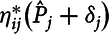 $\eta _{ij}^*\left( {{{\hat P}_j} + {\delta _j}} \right)$ is the utility-constant change in quantity; we replace this with the model output proportionate change in quantity,
  ${\hat Q_j}$. Second, note that
  $${\delta _j}$$ is the proportionate demand shift in the price direction, which in our case is simply the gluten-free flexibility multiplied by the assumed proportionate change in media articles.
Updated data, averaged across years 2004–2017, for annual expenditures for each of the nine food products are provided in Table B2. Values of production used to calculate changes in producer surplus are also averaged across years 2004–2017 (when possible). Values are in Table B3.
Table B1. Compensated own- and cross-price gluten-free flexibilities using iterative seemingly unrelated regressions (ITSUR) estimates of the Inverse Almost Ideal Demand System (IAIDS) model with monthly data

Table B2. Annual food expenditures (million US$)
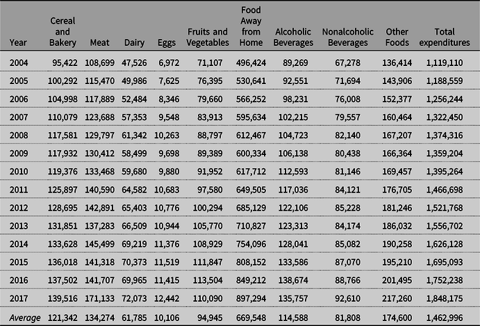
Table B3. Average annual values of production by commodity: 2004–2017 (million US$)


 Open access