


1 Introduction
In a previous paper [Reference Piazza and Pulcini24], two of the current authors introduced an informational refinement of the standard Boolean semantics for classical propositional logic. This account reverses the traditional perspective whereby proof-systems are shown to be sound and complete under a preassigned external semantic structure: primacy is instead accorded to proofs which, through their very combinatorial structure, determine from within the semantic value of logical formulas. The intrinsically finitary notion of derivation makes the nature of such semantics finitary as well, despite the infinitude of its truth-values which are elements of the set of rational numbers
 $\mathbb {Q}$
in the closed interval
$\mathbb {Q}$
in the closed interval
 $[0,1]$
. The most visible upshot of the new treatment is the breaking of the symmetry between classical tautologies and contradictions: the former are uniformly interpreted by the value 1, while the latter become susceptible to different fractional interpretations. This is why we called such semantics “fractional” and we argued that it conforms with the general project of proof-theoretic semantics in considering the classical rules as a medium through which meaning propagates.
$[0,1]$
. The most visible upshot of the new treatment is the breaking of the symmetry between classical tautologies and contradictions: the former are uniformly interpreted by the value 1, while the latter become susceptible to different fractional interpretations. This is why we called such semantics “fractional” and we argued that it conforms with the general project of proof-theoretic semantics in considering the classical rules as a medium through which meaning propagates.
Fractional semantics, however, requires an appropriate proof-theoretic platform within which it can be articulated. Namely, in order to allow for a fractional interpretation of its formulas, a decidable logic
 $\mathscr {L}$
needs to be displayed in a sequent system
$\mathscr {L}$
needs to be displayed in a sequent system
 $\mathsf {S}$
(or its variants) meeting three conditions:
$\mathsf {S}$
(or its variants) meeting three conditions:
-
(1) Bilateralism:
 $\mathsf {S}$
proves all the valid formulas of
$\mathscr {L}$
and refutes all the invalid ones through logical rules involving both deduction and refutation [Reference Bendall4, Reference Francez10, Reference Pulcini, Varzi and Fitting28, Reference Rumfitt29, Reference Wansing35]. In other words,
$\mathsf {S}$
, as a bilateral system, generates
$\mathsf {S}$
-derivations for any well-formed formula A of
$\mathscr {L}$
: if A is valid, its
$\mathsf {S}$
-derivation will be an actual proof of A; if A is invalid, its
$\mathsf {S}$
-derivation will provide a formal refutation of A, i.e., a proof of its unprovability.Footnote
1
$\mathsf {S}$
proves all the valid formulas of
$\mathscr {L}$
and refutes all the invalid ones through logical rules involving both deduction and refutation [Reference Bendall4, Reference Francez10, Reference Pulcini, Varzi and Fitting28, Reference Rumfitt29, Reference Wansing35]. In other words,
$\mathsf {S}$
, as a bilateral system, generates
$\mathsf {S}$
-derivations for any well-formed formula A of
$\mathscr {L}$
: if A is valid, its
$\mathsf {S}$
-derivation will be an actual proof of A; if A is invalid, its
$\mathsf {S}$
-derivation will provide a formal refutation of A, i.e., a proof of its unprovability.Footnote
1
-
(2) Invertibility: each logical rule of
$\mathsf {S}$
is invertible, meaning that the provability of its conclusion implies the provability of (each one of) its premise(s) [Reference Ketonen16]. This means that proof-search in
$\mathsf {S}$
boils down to an algorithm for decomposing any given sequent into an equivalent multiset of clauses which includes exactly the top-sequents (valid or invalid) of the achieved proof. By such a proof-as-decomposing setting, every
$\mathsf {S}$
-derivation
$\pi $
ending with A shapes a numerical evaluation
$\big [\!\big [ A\big ]\!\big ]$
of A. To be more precise,
$\big [\!\big [ A\big ]\!\big ]$
is expressed in terms of the ratio between the number of
$\pi $
’s valid top-sequents and the total number of top-sequents. -
(3) Stability: two analytic
$\mathsf {S}$
-proofs with the same end-sequent share the same multiset of top-sequents. This property ensures that fractional evaluations accommodate the demands of an effective semantics: because (bottom-up) proof-search generates a certain multiset of top-sequents, stability can refer directly to such multiset associated with any formula of
$\mathscr {L}$
.


In sum: on the fractional view, proving a certain sentence A amounts to measuring the quantity of validity involved in A, relative to A’s decomposition into elementary top-sequents. In [Reference Piazza and Pulcini24] the adopted system for classical propositional logic was the bilateral version of Kleene’s sequent calculus
 $\mathsf {G4}$
[Reference Kleene17, Reference Troelstra and Schwichtenberg30], called
$\mathsf {G4}$
[Reference Kleene17, Reference Troelstra and Schwichtenberg30], called
 $\overline {\overline {\mathsf {G4}}}$
, and satisfying both the invertibility and stability properties. By way of example, in
$\overline {\overline {\mathsf {G4}}}$
, and satisfying both the invertibility and stability properties. By way of example, in
 $\overline {\overline {\mathsf {G4}}}$
the classical contradiction
$\overline {\overline {\mathsf {G4}}}$
the classical contradiction
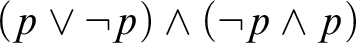 $(p\vee \neg p)\wedge (\neg p\wedge p)$
is thus derivable:
$(p\vee \neg p)\wedge (\neg p\wedge p)$
is thus derivable:

The
 $\overline {\overline {\mathsf {G4}}}$
-derivation above qualifies as a disproof of
$\overline {\overline {\mathsf {G4}}}$
-derivation above qualifies as a disproof of
 $(p\vee \neg p)\wedge (\neg p\wedge p)$
and, insofar as it contains only one tautological clause out of three top-sequents in total,
$(p\vee \neg p)\wedge (\neg p\wedge p)$
and, insofar as it contains only one tautological clause out of three top-sequents in total,
 $\big [\!\big [ (p\vee \neg p)\wedge (\neg p\wedge p)\big ]\!\big ]=\displaystyle \displaystyle {}^{1}\!/_{3}=0.\overline {3}$
. Stability intervenes to guarantee that any other possible
$\big [\!\big [ (p\vee \neg p)\wedge (\neg p\wedge p)\big ]\!\big ]=\displaystyle \displaystyle {}^{1}\!/_{3}=0.\overline {3}$
. Stability intervenes to guarantee that any other possible
 $\overline {\overline {\mathsf {G4}}}$
-derivation of
$\overline {\overline {\mathsf {G4}}}$
-derivation of
 $\Rightarrow (p\vee \neg p)\wedge (\neg p\wedge p)$
will always return the value
$\Rightarrow (p\vee \neg p)\wedge (\neg p\wedge p)$
will always return the value
 $0.\overline {3}$
.
$0.\overline {3}$
.
In this paper, we aim at expanding this fractional account to modal logic by designing a modal proof-system constrained by bilateralism, invertibility, and stability. Notoriously, the inadequacy of a truth-functional approach to modal logic was established by Dugundji’s celebrated result in 1940, according to which Lewis systems from
 $S1$
to
$S1$
to
 $S5$
cannot be semantically characterized by an n-valued semantics [Reference Coniglio and Peron8, Reference Dugundji9]. Still, many well-known modal systems such as K, T,
$S5$
cannot be semantically characterized by an n-valued semantics [Reference Coniglio and Peron8, Reference Dugundji9]. Still, many well-known modal systems such as K, T,
 $4$
, B,
$4$
, B,
 $GL$
, and
$GL$
, and
 $S1\text {-}5$
are decidable and satisfy the finite model property [Reference Chagrov and Zakharyaschev7]. Furthermore, in the past two decades many of the above systems have received a satisfactory proof-theoretic treatment and for each of them different frameworks of proof systems have been furnished.
$S1\text {-}5$
are decidable and satisfy the finite model property [Reference Chagrov and Zakharyaschev7]. Furthermore, in the past two decades many of the above systems have received a satisfactory proof-theoretic treatment and for each of them different frameworks of proof systems have been furnished.
Initially this treatment attained cut-free and decidable sequent calculi, but failed to encompass modal systems such as B or
 $S5$
, where the axiom corresponding to symmetry proved to be very hard to handle. The picture changed when suitable generalizations of the classical sequent calculus entered the scene. These new frameworks were presented in two different fashions: either via the internalization of semantics [Reference Negri22, Reference Viganò31], or by enriching the structure of sequents [Reference Avron, Hodges, Hyland, Steinhorn and Truss3, Reference Brünnler6, Reference Poggiolesi26]. Both these approaches allowed for the formulation of proof-systems with good structural properties and, in most cases, yielding well-defined decision procedures. In sum, the quest for a well-behaved Gentzen-style proof theory has progressively brought modal logics closer to classical logic by recovering proof-theoretic properties such as symmetry and harmony which typically characterize sequent calculi for classical logic.
$S5$
, where the axiom corresponding to symmetry proved to be very hard to handle. The picture changed when suitable generalizations of the classical sequent calculus entered the scene. These new frameworks were presented in two different fashions: either via the internalization of semantics [Reference Negri22, Reference Viganò31], or by enriching the structure of sequents [Reference Avron, Hodges, Hyland, Steinhorn and Truss3, Reference Brünnler6, Reference Poggiolesi26]. Both these approaches allowed for the formulation of proof-systems with good structural properties and, in most cases, yielding well-defined decision procedures. In sum, the quest for a well-behaved Gentzen-style proof theory has progressively brought modal logics closer to classical logic by recovering proof-theoretic properties such as symmetry and harmony which typically characterize sequent calculi for classical logic.
In what follows we will be concerned with the normal modal logic K, that is the minimal modal system including the K-axiom
![]() and closed under the rule of necessitation: if A is a theorem, so is
and closed under the rule of necessitation: if A is a theorem, so is
![]() . K represents a base for the other modal systems—obtained via the addition of specific axioms—in which the modality gains more and more sophisticated interpretations. Moreover, our perspective also involves an attempt to develop a proof-theoretic semantics for modal logic by building a bridge between modal and classical logic. Indeed, we subscribe to the claim that proof-theoretic semantics is “seriously incomplete” without an account of the meanings of modal operators in terms of rules of inference [Reference Kürbis18, p. 724]. There is, however, an important methodological difference between the approach here proposed and the more standard ones [Reference Francez11, Reference Piecha and Schroeder-Heister25, Reference Wansing32]. Traditional stances share the view that the meaning of logical operators should be transmitted by the rules governing their use. This is an essentially local approach in the sense that single inference steps are taken to convey an operational interpretation irrespective of the specific formal proof in which inferences occur. In the context of fractional semantics, by contrast, the approach we are pursuing can be classified as global: it appeals, indeed, to the macro-structure of proofs determining the decomposition of formulas and, consequently, to the multiset of clauses displayed as top-sequents. Single inferences still contribute to meaning but, so we argue, the latter can be fully extracted only from the proof as an organic unity.
. K represents a base for the other modal systems—obtained via the addition of specific axioms—in which the modality gains more and more sophisticated interpretations. Moreover, our perspective also involves an attempt to develop a proof-theoretic semantics for modal logic by building a bridge between modal and classical logic. Indeed, we subscribe to the claim that proof-theoretic semantics is “seriously incomplete” without an account of the meanings of modal operators in terms of rules of inference [Reference Kürbis18, p. 724]. There is, however, an important methodological difference between the approach here proposed and the more standard ones [Reference Francez11, Reference Piecha and Schroeder-Heister25, Reference Wansing32]. Traditional stances share the view that the meaning of logical operators should be transmitted by the rules governing their use. This is an essentially local approach in the sense that single inference steps are taken to convey an operational interpretation irrespective of the specific formal proof in which inferences occur. In the context of fractional semantics, by contrast, the approach we are pursuing can be classified as global: it appeals, indeed, to the macro-structure of proofs determining the decomposition of formulas and, consequently, to the multiset of clauses displayed as top-sequents. Single inferences still contribute to meaning but, so we argue, the latter can be fully extracted only from the proof as an organic unity.
On the other hand, fractional semantics affords an informational refinement of modal logic, in which, like in classical logic, the notion of validity is traditionally interpreted as a sharp one, without some degree of truth or validity. It is important to appreciate, however, that analyticity and invertibility of the calculus weed out any suspicion that such an informational refinement is an arbitrary one. Indeed, the decomposition induced by the rules of the calculus reduces the validity (or invalidity) of the end-sequent to the validity (or invalidity) of the top-sequents. So, every branch of a derivation terminating in a non-axiomatic sequent may be understood as a successful attempt at falsifying the end-sequent. Therefore, the ratio between axiomatic and complementary sequents determines the degree of validity of a formula. In particular, this refinement enables us to propose a novel proof of Dugundji’s theorem, relative to K, which gets rid of the construction of an infinite countermodel.
Our proof-theoretic machinery comes as a bilateral hypersequent calculus for K; as far as we know, this is the first calculus of this type for some systems of modal logic in the literature. Moreover, as well as being a deductive setting in which fractional semantics can be implemented, this system has an intrinsic proof-theoretic interest to the extent that it reconciles the invertibility of the rules (thus eliminating the need for backtracking) with the finiteness of the proof-search space. As a matter of fact, the standard sequent calculus for modal logic K [Reference Wansing, Gabbay and Guenthner33] satisfies termination, but it essentially requires a backtracking procedure due to the failure of invertibility. Vice versa, extensions of the standard framework of sequent calculus such as labeled sequent calculi [Reference Negri22], nested sequents [Reference Brünnler6], or display calculi [Reference Wansing34] enjoy full invertibility, but the proof-search space is not finite.
The plan of the paper is as follows. In Section 2, we first introduce the proof-system
 $\overline {\overline {\mathsf {HK}}}$
, a bilateral hypersequent calculus sound and complete with respect to the set of K-valid formulas.
$\overline {\overline {\mathsf {HK}}}$
, a bilateral hypersequent calculus sound and complete with respect to the set of K-valid formulas.
 $\overline {\overline {\mathsf {HK}}}$
is shown to satisfy some desirable structural properties, including the invertibility of the logical rules and cut-elimination. In Section 3, we establish stability and, contextually, we show how to employ
$\overline {\overline {\mathsf {HK}}}$
is shown to satisfy some desirable structural properties, including the invertibility of the logical rules and cut-elimination. In Section 3, we establish stability and, contextually, we show how to employ
 $\overline {\overline {\mathsf {HK}}}$
as an algorithm to fractionally evaluate K-formulas. Then, in Section 4, such a fractional interpretation becomes a lens through which we closer look at Dugundji’s theorem. Finally, Section 5 offers some concluding remarks.
$\overline {\overline {\mathsf {HK}}}$
as an algorithm to fractionally evaluate K-formulas. Then, in Section 4, such a fractional interpretation becomes a lens through which we closer look at Dugundji’s theorem. Finally, Section 5 offers some concluding remarks.
2 An invertible bilateral hypersequent calculus for K
2.1 The calculus
$\overline {\overline {\mathsf {HK}}}$

We shall be mainly working with hypersequents, introduced under a different name by Mints in the early seventies of the last century [Reference Mints20, Reference Mints21] and independently by Pottinger [Reference Pottinger27], then further elaborated (and so named) by Avron [Reference Avron1–Reference Avron, Hodges, Hyland, Steinhorn and Truss3]. They are a generalization of the standard notion of sequent in the style of Gentzen. A sequent is a syntactic entity of the form
 $\Gamma \Rightarrow \Delta $
, where
$\Gamma \Rightarrow \Delta $
, where
 $\Gamma ,\Delta $
are finite multisets of modal formulas from the set
$\Gamma ,\Delta $
are finite multisets of modal formulas from the set
 $\mathscr {F}$
recursively defined by the grammar:
$\mathscr {F}$
recursively defined by the grammar:
with
 $AT$
collecting the atomic sentences. As usual,
$AT$
collecting the atomic sentences. As usual,
 $\lozenge A$
abridges the formula
$\lozenge A$
abridges the formula
. If
 $\Gamma =[A_{1},A_{2},\ldots ,A_{n}]$
, then
$\Gamma =[A_{1},A_{2},\ldots ,A_{n}]$
, then
 $\bigwedge \Gamma $
and
$\bigwedge \Gamma $
and
 $\bigvee \Gamma $
are the two formulas
$\bigvee \Gamma $
are the two formulas
 $A_{1}\wedge A_{2}\wedge \cdots \wedge A_{n}$
and
$A_{1}\wedge A_{2}\wedge \cdots \wedge A_{n}$
and
 $A_{1}\vee A_{2}\vee \cdots \vee A_{n}$
, respectively. If
$A_{1}\vee A_{2}\vee \cdots \vee A_{n}$
, respectively. If
 $\Gamma =\varnothing $
, then we set
$\Gamma =\varnothing $
, then we set
 $\bigwedge \Gamma =\top $
and
$\bigwedge \Gamma =\top $
and
 $\bigvee \Gamma =\bot $
, where
$\bigvee \Gamma =\bot $
, where
 $\top $
and
$\top $
and
 $\bot $
stand for an arbitrarily selected tautology and contradiction, respectively. With
$\bot $
stand for an arbitrarily selected tautology and contradiction, respectively. With
we mean the multiset
. For every formula A we denote with
 $A^{n}$
the multiset containing exactly n occurrences of A.
$A^{n}$
the multiset containing exactly n occurrences of A.
In general, if M and N are two multisets, we indicate with
 $M\uplus N$
and
$M\uplus N$
and
 $\#M$
their multiset union and M’s cardinality, respectively. A hypersequent, denoted by
$\#M$
their multiset union and M’s cardinality, respectively. A hypersequent, denoted by
 $\mathcal {G},\mathcal {H},\ldots $
, is defined as a finite (possibly empty) multiset of sequents written as follows:
$\mathcal {G},\mathcal {H},\ldots $
, is defined as a finite (possibly empty) multiset of sequents written as follows:
 $$ \begin{align*}\Gamma_{1}\Rightarrow\Delta_{1}\,|\,\Gamma_{2}\Rightarrow\Delta_{2}\,|\,\cdots\,|\,\Gamma_{n}\Rightarrow\Delta_{n}.\end{align*} $$
We shall keep calling “sequents” those hypersequents listing exactly one sequent. The set collecting hypersequents is here indicated with
 $\mathscr {H}$
. Informally speaking, a hypersequent
$\mathscr {H}$
. Informally speaking, a hypersequent
 $\mathcal {G}$
proves valid whenever at least one of the sequents listed in
$\mathcal {G}$
proves valid whenever at least one of the sequents listed in
 $\mathcal {G}$
is valid. Here the meaning of the term “valid” has to be specified depending on the logical context (cf. Definition 3).
$\mathcal {G}$
is valid. Here the meaning of the term “valid” has to be specified depending on the logical context (cf. Definition 3).
The following definition introduces the notion of hyperclause which extends that of clause for standard sequents of classical logic.
Definition 1 (Hyperclauses)
A hyperclause is a hypersequent
such that
 $\Gamma _{i}\uplus \Delta _{i}\subset AT$
, for all
$\Gamma _{i}\uplus \Delta _{i}\subset AT$
, for all
 $1\leqslant i\leqslant n$
. An identity hyperclause is such that, for some i,
$1\leqslant i\leqslant n$
. An identity hyperclause is such that, for some i,
 $\Gamma _{i}\uplus \Delta _{i}\neq \varnothing $
; otherwise, it is complementary.
$\Gamma _{i}\uplus \Delta _{i}\neq \varnothing $
; otherwise, it is complementary.
Example 2.1. An identity hyperclause and a complementary hyperclause, respectively:
Figure 1 presents the bilateral hypersequent calculus
 $\overline {\overline {\mathsf {HK}}}$
. The rules of
$\overline {\overline {\mathsf {HK}}}$
. The rules of
 $\overline {\overline {\mathsf {HK}}}$
operate on hypersequents signed with the symbols “
$\overline {\overline {\mathsf {HK}}}$
operate on hypersequents signed with the symbols “
 $\vdash $
” and “
$\vdash $
” and “
 $\dashv $
”: we write
$\dashv $
”: we write
 $\vdash \mathcal {G}$
and
$\vdash \mathcal {G}$
and
 $\dashv \mathcal {G}$
to assert the validity and invalidity of
$\dashv \mathcal {G}$
to assert the validity and invalidity of
 $\mathcal {G}$
, respectively (cf. Definition 3). For the sake of a more compact notation, in Figure 1 the
$\mathcal {G}$
, respectively (cf. Definition 3). For the sake of a more compact notation, in Figure 1 the
 $\overline {\overline {\mathsf {HK}}}$
rules are expressed by writing
$\overline {\overline {\mathsf {HK}}}$
rules are expressed by writing
![]() and
and
![]() to indicate the two signs “
to indicate the two signs “
 $\vdash $
” and “
$\vdash $
” and “
 $\dashv $
,” respectively. The calculus is equipped with two axiom rules: the
$\dashv $
,” respectively. The calculus is equipped with two axiom rules: the
 $ax$
-rule introduces any identity hyperclause, whilst the
$ax$
-rule introduces any identity hyperclause, whilst the
 $\overline {ax}$
-rule introduces whatsoever complementary hyperclause.
$\overline {ax}$
-rule introduces whatsoever complementary hyperclause.

Fig. 1 The
 $\overline {\overline {\mathsf {HK}}}$
sequent calculus (read
$\overline {\overline {\mathsf {HK}}}$
sequent calculus (read
![]() as
as
 $\vdash $
, and
$\vdash $
, and
![]() as
as
 $\dashv $
).
$\dashv $
).
From now on, we will indicate derivations with small Greek letters
 $\pi ,\rho ,\ldots $
. The height
$\pi ,\rho ,\ldots $
. The height
 $h(\pi )$
of a derivation
$h(\pi )$
of a derivation
 $\pi $
is given by the number of hypersequents figuring in one of its longest branches. Moreover, we indicate with
$\pi $
is given by the number of hypersequents figuring in one of its longest branches. Moreover, we indicate with
 $\mathsf {top}(\pi )$
the multiset of
$\mathsf {top}(\pi )$
the multiset of
 $\pi $
’s top-hypersequents.
$\pi $
’s top-hypersequents.
Example 2.2.
Figure 2 displays an
 $\overline {\overline {\mathsf {HK}}}$
-derivation ending in
$\overline {\overline {\mathsf {HK}}}$
-derivation ending in
![]() .
.

Fig. 2 An example of
 $\overline {\overline {\mathsf {HK}}}$
proof.
$\overline {\overline {\mathsf {HK}}}$
proof.
Remark 1. The rule
![]() is the only rule in which the hypersequent structure comes effectively into play. Informally speaking, it allows us to separate a classical and a modal part in a derivation. In fact, every time this rule is applied, a new hypersequent component is added, thus starting a parallel derivation.
is the only rule in which the hypersequent structure comes effectively into play. Informally speaking, it allows us to separate a classical and a modal part in a derivation. In fact, every time this rule is applied, a new hypersequent component is added, thus starting a parallel derivation.
Furthermore, notice that the side condition on the
![]() -rule about the two contexts
-rule about the two contexts
 $\Gamma '$
and
$\Gamma '$
and
 $\Delta '$
is crucial to avoid pathological situations in which, for some hypersequent
$\Delta '$
is crucial to avoid pathological situations in which, for some hypersequent
 $\mathcal {G}$
,
$\mathcal {G}$
,
 $\overline {\overline {\mathsf {HK}}}$
proves both
$\overline {\overline {\mathsf {HK}}}$
proves both
 $\vdash \mathcal {G}$
and
$\vdash \mathcal {G}$
and
 $\dashv \mathcal {G}$
as the following:
$\dashv \mathcal {G}$
as the following:

Lemma 2.1. For any hypersequent
 $\mathcal {G}$
,
$\mathcal {G}$
,
 $\overline {\overline {\mathsf {HK}}}$
proves
$\overline {\overline {\mathsf {HK}}}$
proves
 $\vdash \mathcal {G}$
or it proves
$\vdash \mathcal {G}$
or it proves
 $\dashv \mathcal {G}$
.
$\dashv \mathcal {G}$
.
Proof. Any hypersequent which is not a hyperclause can be further analyzed via some suitable bottom-up applications of the rules in which the part concerning the standard/reversed turnstile is simply ignored. Once the decomposition is fully accomplished, we can recover the information about turnstiles by propagating it from the axiom-leaves to the conclusion, according to the rules listed in Figure 1.□
2.2 Bilateral soundness and completeness
Let us begin by briefly recalling some basic semantic notions.
Definition 2 (K-model, K-validity)
A K-model
 $\mathscr {M}$
consists of a triple
$\mathscr {M}$
consists of a triple
 $\langle W, R, v\rangle $
where
$\langle W, R, v\rangle $
where
 $W\neq \varnothing $
,
$W\neq \varnothing $
,
 $R\subseteq W^{2}$
and
$R\subseteq W^{2}$
and
 $v:AT\to \mathcal {P}(W)$
is a valuation function. For every
$v:AT\to \mathcal {P}(W)$
is a valuation function. For every
 $w\in W$
and every formula A, the relation
$w\in W$
and every formula A, the relation
 $w\Vdash A$
is thus defined:
$w\Vdash A$
is thus defined:
-
•
$w\Vdash p$
iff
$w\in v(p)$
for every
$p\in AT$
, -
•
$w\Vdash \neg B$
iff
$w\nVdash B$
, -
•
$w\Vdash B\wedge C$
iff
$w\Vdash B$
and
$w\Vdash C$
, -
•
$w\Vdash B\vee C$
iff
$w\Vdash B$
or
$w\Vdash C$
, -
•
$w\Vdash B\to C$
iff if
$w\nVdash B$
or
$w\Vdash C$
, -
•
iff for every
$w'$
, if
$Rww'$
, then
$w'\vDash B$
.


The sentence A is true in
 $\mathscr {M}$
iff
$\mathscr {M}$
iff
 $w\Vdash A$
, for all
$w\Vdash A$
, for all
 $w\in W$
. Moreover, A is valid, in symbols
$w\in W$
. Moreover, A is valid, in symbols
 $\vDash A$
, in case it is true in any K-model; otherwise, it is invalid.
$\vDash A$
, in case it is true in any K-model; otherwise, it is invalid.
According to the customary operational interpretation of sequents,
 $\Gamma \Rightarrow \Delta $
is K-valid if the formula
$\Gamma \Rightarrow \Delta $
is K-valid if the formula
 $\bigwedge \Gamma \rightarrow \bigvee \Delta $
is K-valid. The next definition accommodates the notion of K-validity to hypersequents.
$\bigwedge \Gamma \rightarrow \bigvee \Delta $
is K-valid. The next definition accommodates the notion of K-validity to hypersequents.
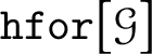
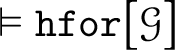
Definition 3 (K-valid hypersequents)
For any hypersequent
 $\mathcal {G}\equiv \Gamma _{1}\Rightarrow \Delta _{1}\,|\, \cdots \,|\,\Gamma _{n}\Rightarrow \Delta _{n}$
, the function
$\mathcal {G}\equiv \Gamma _{1}\Rightarrow \Delta _{1}\,|\, \cdots \,|\,\Gamma _{n}\Rightarrow \Delta _{n}$
, the function
 $\mathtt {hfor}:\mathscr {H}\mapsto \mathscr {F}$
is defined as follows:
$\mathtt {hfor}:\mathscr {H}\mapsto \mathscr {F}$
is defined as follows:

A hypersequent
 $\mathcal {G}$
is said to be K-valid just in case the formula
$\mathcal {G}$
is said to be K-valid just in case the formula
 $\mathtt {hfor}\big [\mathcal {G}\big ]$
is K-valid.
$\mathtt {hfor}\big [\mathcal {G}\big ]$
is K-valid.
Example 2.3. Under Definition 3, the hypersequent
turns out to be K-valid, being valid the following formula:

It should not escape notice that hypersequents cannot be treated naively by interpreting
 $\Gamma _{1}\Rightarrow \Delta _{1} \, |\, \cdots \, |\, \Gamma _{n}\Rightarrow \Delta _{n}$
as the formula
$\Gamma _{1}\Rightarrow \Delta _{1} \, |\, \cdots \, |\, \Gamma _{n}\Rightarrow \Delta _{n}$
as the formula
 $(\bigwedge \Gamma _{1}\to \bigvee \Delta _{1})\lor \cdots \lor (\bigwedge \Gamma _{n}\to \bigvee \Delta _{n})$
. Such an interpretation would make collapse, for instance, the two hypersequents
$(\bigwedge \Gamma _{1}\to \bigvee \Delta _{1})\lor \cdots \lor (\bigwedge \Gamma _{n}\to \bigvee \Delta _{n})$
. Such an interpretation would make collapse, for instance, the two hypersequents
 $\Rightarrow A\vee \neg A$
and
$\Rightarrow A\vee \neg A$
and
 $\Rightarrow A \,|\, A \Rightarrow $
into the same formula
$\Rightarrow A \,|\, A \Rightarrow $
into the same formula
 $A\vee \neg A$
.
$A\vee \neg A$
.
Lemma 2.2. Any identity (resp. complementary) hyperclause is K-valid
 $($
resp. not K-valid).
$($
resp. not K-valid).
Proof. Consider a generic identity hyperclause
 $\mathcal {G}\,|\,\Gamma ,p\Rightarrow \Delta ,p$
. Then, the formula
$\mathcal {G}\,|\,\Gamma ,p\Rightarrow \Delta ,p$
. Then, the formula
![]() is clearly K-valid, and so is the whole formula
is clearly K-valid, and so is the whole formula
 .
.
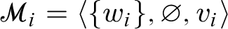
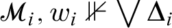
Consider now a complementary hyperclause
![]() . For each sequent
. For each sequent
![]() , take the trivial K-model
, take the trivial K-model
 $\mathscr {M}_{i}=\langle \{w_{i}\}, \varnothing , v_{i}\rangle $
where the interpretation function
$\mathscr {M}_{i}=\langle \{w_{i}\}, \varnothing , v_{i}\rangle $
where the interpretation function
 $v_{i}$
is thus defined:
$v_{i}$
is thus defined:
-
•
$v_{i}(p)=\{w_{i}\}$
, for all
$p\in \Gamma _{i}$
, -
•
$v_{i}(q)=\varnothing $
, for any atom
$q\notin \Gamma _{i}$
.

For every i,
![]() (this is vacuously true by Definition 2) and
(this is vacuously true by Definition 2) and
 $\mathscr {M}_{i},w_{i}\Vdash \bigwedge \Gamma _{i}$
, but
$\mathscr {M}_{i},w_{i}\Vdash \bigwedge \Gamma _{i}$
, but
 $\mathscr {M}_{i},w_{i}\nVdash \bigvee \Delta _{i}$
. Therefore,
$\mathscr {M}_{i},w_{i}\nVdash \bigvee \Delta _{i}$
. Therefore,
![]() . Then, we can easily exhibit the sought countermodel by considering
. Then, we can easily exhibit the sought countermodel by considering
 $$ \begin{align*}\mathscr{M}=\Bigg\langle \{w_{0},w_{1},\ldots,w_{n}\}, \{(w_{0},w_{i})\, |\, 1\leqslant i\leqslant n\}, \hspace{-4pt}\underset{1\leqslant i\leqslant n}{\bigcup} \hspace{-3pt}v_{i}\,\Bigg\rangle.\end{align*} $$
Indeed, for every i, it turns out that
 $Rw_{0}w_{i}$
and
$Rw_{0}w_{i}$
and
![]() , so that we can conclude
, so that we can conclude
 .□
.□
Lemma 2.3 (Modal disjunction property)
If
![]() , then
, then
 $\vDash A$
or
$\vDash A$
or
 $\vDash B$
.
$\vDash B$
.
Proof. The reader is referred to [Reference Chagrov and Zakharyaschev7, pp. 90–91].□
Theorem 2.4 (Soundness)
If the system
 $\overline {\overline {\mathsf {HK}}}$
proves
$\overline {\overline {\mathsf {HK}}}$
proves
 $\vdash \mathcal {G}$
and
$\vdash \mathcal {G}$
and
 $\dashv \mathcal {H}$
, then the hypersequents
$\dashv \mathcal {H}$
, then the hypersequents
 $\mathcal {G}$
and
$\mathcal {G}$
and
 $\mathcal {H}$
are K-valid and K-invalid, respectively.
$\mathcal {H}$
are K-valid and K-invalid, respectively.
Proof. The proof is carried out by induction on the height of a generic
 $\overline {\overline {\mathsf {HK}}}$
-proof
$\overline {\overline {\mathsf {HK}}}$
-proof
 $\pi $
. Lemma 2.2 immediately supplies the base case. As for the inductive case, we limit ourselves to discussing the case in which
$\pi $
. Lemma 2.2 immediately supplies the base case. As for the inductive case, we limit ourselves to discussing the case in which
 $\pi $
’s last inference step is an application of the
$\pi $
’s last inference step is an application of the
![]() -rule. We distinguish two cases according to whether
-rule. We distinguish two cases according to whether
 $\pi $
ends in
$\pi $
ends in
 $\vdash \mathcal {G}$
or
$\vdash \mathcal {G}$
or
 $\dashv \mathcal {H}$
.
$\dashv \mathcal {H}$
.
-
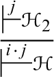
• (
$\vdash \mathcal {G}$
). By inductive hypothesis, it results that the premise
is K-valid, where
$\Gamma ',\Delta '\subset AT$
. In case
$\mathtt {hfor}\big [\mathcal {G}'\big ]$
is a K-valid formula, we immediately get the desired conclusion. Otherwise, by Lemma 2.3, at least one of the two formulas
$\bigwedge \Gamma \to A$
and
turns out to be K-valid: in both cases the conclusion easily follows from the monotonicity of
. -
• (
$\dashv \mathcal {H}$
). According to our inductive hypothesis, the hypersequent
(with
$\Gamma ',\Delta '\subset AT$
and
$\Gamma '\cap \Delta '=\varnothing $
) is now taken to be K-invalid. Consider the hypersequent
$\mathcal {G} \equiv \Pi _{1}\Rightarrow \Sigma _{1}\, |\, \cdots \, |\, \Pi _{n}\Rightarrow \Sigma _{n}$
and let i and j be two parameters ranging over the sets
$\{1,\ldots ,n\}$
and
$\{1,\ldots ,n+2\}$
, respectively. Clearly, none of the formulas
$\bigwedge \Pi _{i}\rightarrow \bigvee \Delta _{i}$
is K-valid. The two formulas,
and
$\bigwedge \Gamma \rightarrow A$
, are not K-valid as well. This means that there is a family of models
$\mathscr {M}_{j}=\langle W_{j}, R_{j}, v_{j}\rangle $
such that:-
(1)
$\langle W_{j}, R_{j}\rangle $
is a irreflexive, asymmetric, and intransitive tree with root
$w_{j}$
[Reference Blackburn, de Rijke and Venema5, p. 218], -
(2)
$\mathscr {M}_{i},w_{i}\Vdash \bigwedge \Pi _{i}$
and
$\mathscr {M}_{i},w_{i}\nVdash \bigvee \Sigma _{i}$
, -
(3)
and
, -
(4)
$\mathscr {M}_{n+2},w_{n+2}\Vdash \bigwedge \Gamma $
and
$\mathscr {M}_{n+2},w_{n+2}\,\nVdash A$
.
Thus, finally consider the model
and observe that
$$ \begin{align*} \mathscr{M}&=\Bigg\langle \,\overset{n + 2}{\underset{j= 1}{\bigcup}} W_{j}\cup\{w_{0}\}, \,\, \overset{n+2}{\underset{j=1}{\bigcup}}R_{j}\cup\Big\{(w_{n+1},w_{n+2})\Big\}\\ &\qquad\cup \Big\{(w_{0},w_{k})\, |\, 1\leqslant k\leqslant n+1\Big\}, \,\, \overset{n+2}{\underset{j=1}{\bigcup}} v_{j} \Bigg\rangle \end{align*} $$
which yields the desired conclusion. (Let us observe that the constraint
$\Gamma ',\Delta '\subset AT$
is essential in the final part of the previous argument to prevent that
$\mathscr {M},x_{n+1}\nVdash \bigwedge \Gamma '$
by adding
$R (w_{n+1},w_{n+2})$
to the model).□
-


Corollary 2.5 (Completeness)
If the hypersequent
 $\mathcal {G}$
is K-valid, then
$\mathcal {G}$
is K-valid, then
 $\overline {\overline {\mathsf {HK}}}$
proves
$\overline {\overline {\mathsf {HK}}}$
proves
 $\vdash \mathcal {G}$
. Otherwise,
$\vdash \mathcal {G}$
. Otherwise,
 $\overline {\overline {\mathsf {HK}}}$
proves
$\overline {\overline {\mathsf {HK}}}$
proves
 $\dashv \mathcal {G}$
.
$\dashv \mathcal {G}$
.
Proof. Assume that
 $\mathcal {G}$
is K-valid, but
$\mathcal {G}$
is K-valid, but
 $\overline {\overline {\mathsf {HK}}}$
does not prove
$\overline {\overline {\mathsf {HK}}}$
does not prove
 $\vdash \mathcal {G}$
. By Lemma 2.1,
$\vdash \mathcal {G}$
. By Lemma 2.1,
 $\overline {\overline {\mathsf {HK}}}$
proves
$\overline {\overline {\mathsf {HK}}}$
proves
 $\dashv \mathcal {G}$
and so, by Theorem 2.4,
$\dashv \mathcal {G}$
and so, by Theorem 2.4,
 $\mathcal {G}$
would be K-invalid. Therefore,
$\mathcal {G}$
would be K-invalid. Therefore,
 $\overline {\overline {\mathsf {HK}}}$
does prove
$\overline {\overline {\mathsf {HK}}}$
does prove
 $\vdash \mathcal {G}$
. The case in which
$\vdash \mathcal {G}$
. The case in which
 $\mathcal {G}$
is K-invalid can be treated symmetrically.□
$\mathcal {G}$
is K-invalid can be treated symmetrically.□
Let us call
 $\mathsf {HK}$
the hypersequent system obtained from
$\mathsf {HK}$
the hypersequent system obtained from
 $\overline {\overline {\mathsf {HK}}}$
by dropping the complementary axiom and removing everywhere the signs “
$\overline {\overline {\mathsf {HK}}}$
by dropping the complementary axiom and removing everywhere the signs “
 $\vdash $
” and “
$\vdash $
” and “
 $\dashv $
.” What we get in this way is a complete “monolateral” characterization of the system K. More formally:
$\dashv $
.” What we get in this way is a complete “monolateral” characterization of the system K. More formally:
Theorem 2.6.
 $\mathsf {HK}$
proves
$\mathsf {HK}$
proves
 $\Rightarrow A$
if and only if
$\Rightarrow A$
if and only if
 $\vDash A$
.
$\vDash A$
.
Proof. Any proof in which no application of the complementary axiom occurs will necessarily end with a hypersequent signed with “
 $\vdash $
.” Then, by Theorem 2.4, the formula
$\vdash $
.” Then, by Theorem 2.4, the formula
![]() is valid and, by the rule of denecessitation (from
is valid and, by the rule of denecessitation (from
![]() to
to
 $\vDash A$
), we finally get the claim of the theorem.□
$\vDash A$
), we finally get the claim of the theorem.□
Remark 2. The rule of denecessitation is indeed sound in K, but it does not prove admissible in every modal system, for example
 $K5$
. Therefore, in order to extend the fractional interpretation to such systems a new strategy would be required.
$K5$
. Therefore, in order to extend the fractional interpretation to such systems a new strategy would be required.
Corollary 2.7. The bilateral cut rule:

is admissible in
 $\overline {\overline {\mathsf {HK}}}$
.
$\overline {\overline {\mathsf {HK}}}$
.
Proof. We observe that the above-mentioned bilateral rendition of the cut-rule proves sound in
 $\overline {\overline {\mathsf {HK}}}$
. By applying Corollary 2.5 we finally get the claim of the theorem.□
$\overline {\overline {\mathsf {HK}}}$
. By applying Corollary 2.5 we finally get the claim of the theorem.□
In the proof of the next lemma, we will need to employ the notion of principal formula of an inference rule. In case of inference rules introducing one of the classical connectives, the notion of principal formula is just the familiar one (cf. [Reference Troelstra and Schwichtenberg30]). As regards to the rule for
![]() in Figure 1, we take
in Figure 1, we take
![]() to be the principal formula.
to be the principal formula.
Theorem 2.8 (Invertibility)
Each
 $\overline {\overline {\mathsf {HK}}}$
logical rule proves height-bounded invertible with preservation of top-hypersequents, namely:
$\overline {\overline {\mathsf {HK}}}$
logical rule proves height-bounded invertible with preservation of top-hypersequents, namely:
-
(i) for any instance of a unary rule
, if
$\;\overline {\overline {\mathsf {HK}}}$
proves
by way of a proof
$\pi $
, then it also proves
by way of a proof
$\pi _{1}$
such that
$h(\pi _{1})\leqslant h(\pi )$
and
$\mathsf {top}(\pi _{1})=\mathsf {top}(\pi )$
; -
(ii) for any application of a binary rule
, if
$\overline {\overline {\mathsf {HK}}}$
proves
by way of a proof
$\pi $
, then it also proves
and
by way of two proofs
$\pi _{1}$
and
$\pi _{2}$
such that
$h(\pi _{1}),h(\pi _{2})\leqslant h(\pi )$
and
$\mathsf {top}(\pi _{1})\uplus \mathsf {top}(\pi _{2})=\mathsf {top}(\pi )$
.


Proof. We distinguish the cases according to the rule instances. For every rule instance we proceed by induction on the height
 $h(\pi )$
of the derivation
$h(\pi )$
of the derivation
 $\pi $
leading to the end-hypersequent under consideration, and by distinguishing subcases on the basis of the last rule applied. We deal with two rules; the other ones can be treated likewise.
$\pi $
leading to the end-hypersequent under consideration, and by distinguishing subcases on the basis of the last rule applied. We deal with two rules; the other ones can be treated likewise.
-
• (
$\vee \Rightarrow $
) For
$h(\pi )=1$
, the claim holds vacuously. If
$h(\pi )>1$
and the principal formula of
$\pi $
’s last rule occurs in the context of the end-hypersequent, then the conclusion follows by applying the inductive hypothesis to the premise(s) and then the same rule again. If
$h(\pi )>1$
and the last rule applied acted in the component that we are considering, then it cannot be a
-rule due to context restrictions. We limit ourselves to treat the case in which the last inference is a
$(\Rightarrow \land )$
-rule.By applying our inductive hypothesis, we obtain the following four derivations:
with
$i_{1}\cdot i_{2}=i$
and
$j_{1}\cdot j_{2}=j$
, that we recombine as follows:with
$(i_{1}\cdot j_{1})\cdot (i_{2}\cdot j_{2})=i\cdot j$
. Finally, we observe that
$\mathsf {top}(\pi _{1})=\mathsf {top}(\rho _{1})\uplus \mathsf {top}(\rho _{1}'')$
and
$\mathsf {top}(\pi _{2})=\mathsf {top}(\rho _{2}')\uplus \mathsf {top}(\rho _{2}'')$
. From these two facts we can easily derive
$\mathsf {top}(\pi )=\mathsf {top}(\pi ')\uplus \mathsf {top}(\pi '')$
. -
• (
) For
$h(\pi )=1$
, the claim holds vacuously. If
$h(\pi )>1$
and the principal formula occurs in the context of the end-hypersequent, then, as in the previous case, the conclusion follows by applying the inductive hypothesis to the premise(s) and then the same rule again. If
$h(\pi )> 1$
and the last rule acted in the component under consideration, then it will be a
-rule. If the principal formula of the rule instance coincides with the principal formula of the application of the
-rule, the claim clearly holds. Otherwise, we are in the following situation:where, clearly,
$\mathsf {top}(\pi _{1})=\mathsf {top}(\pi )$
. We can now apply our inductive hypothesis so as to get a derivation
$\rho $
of
such that
$\mathsf {top}(\rho )=\mathsf {top}(\pi _{1})$
and
$h(\rho )\leqslant h(\pi _{1})$
. A final application of the
-rule yields the desired result.□


Proposition 2.9. For any
 $\overline {\overline {\mathsf {HK}}}$
-proof
$\overline {\overline {\mathsf {HK}}}$
-proof
 $\pi $
ending in the hypersequent
$\pi $
ending in the hypersequent
 $\mathcal {G}$
and such that
$\mathcal {G}$
and such that
 $\mathsf {top}(\pi )=\big \{\mathcal {T}_{1},\mathcal {T}_{2},\ldots ,\mathcal {T}_{n}\big \}$
, the two formulas
$\mathsf {top}(\pi )=\big \{\mathcal {T}_{1},\mathcal {T}_{2},\ldots ,\mathcal {T}_{n}\big \}$
, the two formulas
 $\mathtt {hfor}\big [\mathcal {G}\big ]$
and
$\mathtt {hfor}\big [\mathcal {G}\big ]$
and
 $\hspace {-6pt}\bigwedge \limits _{1\leqslant i\leqslant n} \hspace {-6pt}\mathtt {hfor}\big [\mathcal {T}_{i}\big ]$
are equivalent, i.e.,
$\hspace {-6pt}\bigwedge \limits _{1\leqslant i\leqslant n} \hspace {-6pt}\mathtt {hfor}\big [\mathcal {T}_{i}\big ]$
are equivalent, i.e.,
 $\vDash \mathtt {hfor}\big [\mathcal {G}\big ]$
if, and only if,
$\vDash \mathtt {hfor}\big [\mathcal {G}\big ]$
if, and only if,
 $\vDash \hspace {-6pt}\bigwedge \limits _{1\leqslant i\leqslant n}\hspace {-6pt}\mathtt {hfor}\big [\mathcal {T}_{i}\big ]$
.
$\vDash \hspace {-6pt}\bigwedge \limits _{1\leqslant i\leqslant n}\hspace {-6pt}\mathtt {hfor}\big [\mathcal {T}_{i}\big ]$
.
Proof. By the soundness theorem we know that, for each logical rule, the conclusion is K-valid just in case the premise(s) is(are) K-valid as well. Thus, it immediately follows that
 $\vDash \mathtt {hfor}\big [\mathcal {G}\big ]$
if, and only if,
$\vDash \mathtt {hfor}\big [\mathcal {G}\big ]$
if, and only if,
 $\vDash \hspace {-8pt}\bigwedge \limits _{1\leqslant i\leqslant n} \hspace {-6pt}\mathtt {hfor}\big [\mathcal {T}_{i}\big ]$
.□
$\vDash \hspace {-8pt}\bigwedge \limits _{1\leqslant i\leqslant n} \hspace {-6pt}\mathtt {hfor}\big [\mathcal {T}_{i}\big ]$
.□
Theorem 2.10. The following statements hold:
-
(1)
$\overline {\overline {\mathsf {HK}}}$
proves
if, and only if,
$\overline {\overline {\mathsf {HK}}}$
proves
with
$\Gamma \uplus \Delta \subset AT$
. -
(2) If
$\overline {\overline {\mathsf {HK}}}$
proves
with
$\mathcal {G}\neq \varnothing $
, then
$\overline {\overline {\mathsf {HK}}}$
proves
.


Proof. We discuss the two items separately.
-
(1) We argue by induction on the height of derivations. From right to left the proof is quite straightforward. As for the left-to-right direction, we proceed as follows. If
$n=0$
, then
is either an instance of
$ax$
or of
$\overline {ax}$
, and so is
$\mathcal {G}\,|\, \Gamma \hspace {-2pt}\Rightarrow \Delta $
. If
$n>0$
the proof follows by applying the inductive hypothesis to the premises of the last rule of the derivation, as no formula in
$\square \Gamma ',\Gamma \hspace {-2pt}\Rightarrow \Delta $
is principal due to the design of the rules. -
(2) If
$\overline {\overline {\mathsf {HK}}}$
proves
, then, by the previous item, it also proves
. Moreover,
$\overline {\overline {\mathsf {HK}}}$
proves
if and only if
is also provable, thus we obtain the desired conclusion.□


As a consequence of Proposition 2.9 and Theorem 2.10, the calculus
 $\overline {\overline {\mathsf {HK}}}$
allows us to reduce the validity (invalidity) of a given end-hypersequent to the validity (invalidity) of the conjunction of axiomatic or complementary hyperclauses which contain only atomic sentences.Footnote
2
$\overline {\overline {\mathsf {HK}}}$
allows us to reduce the validity (invalidity) of a given end-hypersequent to the validity (invalidity) of the conjunction of axiomatic or complementary hyperclauses which contain only atomic sentences.Footnote
2
3 Stability and fractional interpretation
3.1 The stability theorem
Our concern now is that of establishing that the system
 $\overline {\overline {\mathsf {HK}}}$
enjoys the stability property, i.e., the fact that any two proofs ending with the same hypersequent always display the same multiset of top-hypersequents. To put it differently, two proofs having the same end-hypersequent may only differ in the specific order in which their logical rules are applied.
$\overline {\overline {\mathsf {HK}}}$
enjoys the stability property, i.e., the fact that any two proofs ending with the same hypersequent always display the same multiset of top-hypersequents. To put it differently, two proofs having the same end-hypersequent may only differ in the specific order in which their logical rules are applied.
Theorem 3.1 (Stability)
If
 $\pi $
and
$\pi $
and
 $\rho $
are two
$\rho $
are two
 $\overline {\overline {\mathsf {HK}}}$
-derivations ending with the same signed hypersequent, then
$\overline {\overline {\mathsf {HK}}}$
-derivations ending with the same signed hypersequent, then
 $\mathsf {top}(\pi )=\mathsf {top}(\rho )$
.
$\mathsf {top}(\pi )=\mathsf {top}(\rho )$
.
Proof. We proceed by induction on
 $h(\pi )$
. If
$h(\pi )$
. If
 $h(\pi )=1$
, then
$h(\pi )=1$
, then
 $\pi =\rho $
, and so
$\pi =\rho $
, and so
 $\mathsf {top}(\pi )=\mathsf {top}(\rho )$
. Otherwise, let’s distinguish two cases depending on whether
$\mathsf {top}(\pi )=\mathsf {top}(\rho )$
. Otherwise, let’s distinguish two cases depending on whether
 $\pi $
’s last rule is unary or binary.
$\pi $
’s last rule is unary or binary.
-
• First, consider the situation whereby
$\pi $
’s last inference is an application of a unary rule and let
$\pi _{1}$
indicate
$\pi $
’s subproof ending in
.Clearly,
$\mathsf {top}(\pi _{1})=\mathsf {top}(\pi )$
and
$h(\pi _{1})<h(\pi )$
. By Theorem 2.8, there exists a proof
$\rho _{1}$
of
such that
$\mathsf {top}(\rho _{1})=\mathsf {top}(\rho )$
. By inductive hypothesis, we get
$\mathsf {top}(\pi _{1})=\mathsf {top}(\rho _{1})$
and, lastly,
$\mathsf {top}(\pi )=\mathsf {top}(\rho )$
. -
• Consider now the case in which
$\pi $
’s last inference is an application of a binary rule and
$\pi _{1}$
and
$\pi _{2}$
are the two subproofs of
$\pi $
ending in
and
, respectively.Note that
$\mathsf {top}(\pi _{1})\uplus \mathsf {top}(\pi _{2})=\mathsf {top}(\pi )$
and, clearly,
$h(\pi _{1}),h(\pi _{2})<h(\pi )$
. Next, we apply Theorem 2.8 to
$\rho $
in order to infer the existence of two derivations
$\rho _{1}$
and
$\rho _{2}$
ending, respectively, in
and
, and such that
$\mathsf {top}(\rho _{1})\uplus \mathsf {top}(\rho _{2})=\mathsf {top}(\rho )$
. By inductive hypothesis,
$\mathsf {top}(\rho _{1})\uplus \mathsf {top}(\rho _{2})=\mathsf {top}(\pi _{1})\uplus \mathsf {top}(\pi _{2})$
, thence we conclude that
$\mathsf {top}(\pi )=\mathsf {top}(\rho )$
.□


3.2 Fractional interpretation
Insofar as
 $\overline {\overline {\mathsf {HK}}}$
is a bilateral system satisfying stability, any logical formula A univocally determines a specific multiset of hyperclauses, regardless of the particular proof designed to compute such a multiset. This paves the way for the proof-based semantics proposed below.
$\overline {\overline {\mathsf {HK}}}$
is a bilateral system satisfying stability, any logical formula A univocally determines a specific multiset of hyperclauses, regardless of the particular proof designed to compute such a multiset. This paves the way for the proof-based semantics proposed below.
Definition 4. Given a formula A,
 $\mathsf {top}(A)$
is the multiset of the top-hyperclauses in any of the
$\mathsf {top}(A)$
is the multiset of the top-hyperclauses in any of the
 $\overline {\overline {\mathsf {HK}}}$
-derivations ending in (
$\overline {\overline {\mathsf {HK}}}$
-derivations ending in (
 $\vdash $
or
$\vdash $
or
 $\dashv $
)
$\dashv $
)
 $\Rightarrow A$
. The multiset
$\Rightarrow A$
. The multiset
 $\mathsf {top}(A)$
is partitioned into the two multisets
$\mathsf {top}(A)$
is partitioned into the two multisets
 $\mathsf {top}^{1}(A)$
and
$\mathsf {top}^{1}(A)$
and
 $\mathsf {top}^{0}(A)$
collecting, respectively, all the hyperclauses signed by “
$\mathsf {top}^{0}(A)$
collecting, respectively, all the hyperclauses signed by “
 $\vdash $
” and the hyperclauses signed by “
$\vdash $
” and the hyperclauses signed by “
 $\dashv $
.”
$\dashv $
.”
Definition 5. Let
 $\mathbb {Q}^{\ast }=[0,1]\cap \mathbb {Q}$
, i.e.,
$\mathbb {Q}^{\ast }=[0,1]\cap \mathbb {Q}$
, i.e.,
 $\mathbb {Q}^{\ast }$
is the set of the rational numbers in the closed interval
$\mathbb {Q}^{\ast }$
is the set of the rational numbers in the closed interval
 $[0,1]$
. The evaluation function
$[0,1]$
. The evaluation function
 $\big [\!\big [ \,\cdot \,\big ]\!\big ]:\mathscr {F}\mapsto \mathbb {Q}^{\ast }$
is defined as follows: for any logical formula A,
$\big [\!\big [ \,\cdot \,\big ]\!\big ]:\mathscr {F}\mapsto \mathbb {Q}^{\ast }$
is defined as follows: for any logical formula A,
 $\big [\!\big [ A\big ]\!\big ]=\displaystyle \frac {\#\mathsf {top}^{1}(A)}{\#\mathsf {top}(A)}$
.
$\big [\!\big [ A\big ]\!\big ]=\displaystyle \frac {\#\mathsf {top}^{1}(A)}{\#\mathsf {top}(A)}$
.
Example 3.1. Getting back to the derivation
 $\pi $
proposed in Figure 2, we have:
$\pi $
proposed in Figure 2, we have:

Under Definition 5, we have

. In effect, any
 $\overline {\overline {\mathsf {HK}}}$
-proof ending in
$\overline {\overline {\mathsf {HK}}}$
-proof ending in
displays one identity axiom out of two axioms in total.
Figure 3 lists some other formulas of K together with their corresponding fractional value. For example, below is the proof of
![]() :
:

Fig. 3 Some modal formulas together with their fractional value.

As the proof displays one identity axiom out of three axiom applications in total, we get
 .
.
Theorem 3.2 (Conservativity)
For any formula A,
 $\big [\!\big [ A\big ]\!\big ]=1$
if, and only if,
$\big [\!\big [ A\big ]\!\big ]=1$
if, and only if,
 $\vDash A$
.
$\vDash A$
.
Proof. By Theorem 2.4, any formula A is K-valid just in case
 $\mathsf {top}^{1}(A)=\mathsf {top}(A)$
.□
$\mathsf {top}^{1}(A)=\mathsf {top}(A)$
.□
Notoriously, the lack of truth-functionality is an endemic phenomenon when modalities come into play. It should be observed, however, that in a fractional setting truth-functionality fails already at the very classical level; in this regard, easy examples have been presented in [Reference Piazza and Pulcini24].
Let
 $\mathscr {F}^{c}$
be the language of classical propositional logic. The next theorem establishes the surjectivity of the interpretation function
$\mathscr {F}^{c}$
be the language of classical propositional logic. The next theorem establishes the surjectivity of the interpretation function
 $\big [\!\big [ \,\cdot \,\big ]\!\big ]$
. In particular, we have:
$\big [\!\big [ \,\cdot \,\big ]\!\big ]$
. In particular, we have:
Theorem 3.3. For any
 $q\in \mathbb {Q}^{*}$
:
$q\in \mathbb {Q}^{*}$
:
 $(i)$
there is a formula
$(i)$
there is a formula
 $A\in \mathscr {F}^{c}$
s.t.
$A\in \mathscr {F}^{c}$
s.t.
 $\big [\!\big [ A\big ]\!\big ]=q$
, and
$\big [\!\big [ A\big ]\!\big ]=q$
, and
 $(ii)$
there is a formula
$(ii)$
there is a formula
 $B\in \mathscr {F}-\mathscr {F}^{c}$
s.t.
$B\in \mathscr {F}-\mathscr {F}^{c}$
s.t.
 $\big [\!\big [ B\big ]\!\big ]=q$
.
$\big [\!\big [ B\big ]\!\big ]=q$
.
Proof. Let
 $q=\displaystyle {}^{m}\!/_{n}$
, where
$q=\displaystyle {}^{m}\!/_{n}$
, where
 $m,n\in \mathbb {N}^{+}$
and
$m,n\in \mathbb {N}^{+}$
and
 $m\leqslant n$
.
$m\leqslant n$
.
 $(i)$
Consider the formula
$(i)$
Consider the formula
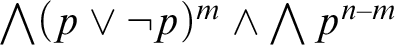 $\bigwedge (p\lor \neg p)^{m}\land \bigwedge p^{n-m}$
. It is immediate to see that
$\bigwedge (p\lor \neg p)^{m}\land \bigwedge p^{n-m}$
. It is immediate to see that
 $\big [\!\big [ \bigwedge (p\lor \neg p)^{m}\land \bigwedge p^{n-m}\big ]\!\big ]=\displaystyle {}^{m}\!/_{n}=q$
.
$\big [\!\big [ \bigwedge (p\lor \neg p)^{m}\land \bigwedge p^{n-m}\big ]\!\big ]=\displaystyle {}^{m}\!/_{n}=q$
.
 $(ii)$
We consider now the modal formula
$(ii)$
We consider now the modal formula
![]() in
in
 $\mathscr {F}-\mathscr {F}^{c}$
. It turns out, similarly, that
$\mathscr {F}-\mathscr {F}^{c}$
. It turns out, similarly, that
 .□
.□
Remark 3. As corollary of Theorem 3.3 and from the density of
 $\mathbb {Q}^{*}$
, it results that for any pair of modal formulas A, B with
$\mathbb {Q}^{*}$
, it results that for any pair of modal formulas A, B with
 $\big [\!\big [ A\big ]\!\big ]< \big [\!\big [ B\big ]\!\big ]$
, there always exists a formula
$\big [\!\big [ A\big ]\!\big ]< \big [\!\big [ B\big ]\!\big ]$
, there always exists a formula
 $C\in \mathscr {F}^{c}$
such that
$C\in \mathscr {F}^{c}$
such that
 $\big [\!\big [ A\big ]\!\big ]< \big [\!\big [ C\big ]\!\big ] < \big [\!\big [ B\big ]\!\big ]$
.
$\big [\!\big [ A\big ]\!\big ]< \big [\!\big [ C\big ]\!\big ] < \big [\!\big [ B\big ]\!\big ]$
.
In a sense, the fractional approach illustrates the continuity between modal logic and classical logic. This claim is strengthened by observing that, in general, for every formula A,
 . However, under fractional semantics modal logic is not monotone, unlike classical logic. To witness this fact, consider the formula
![]() , which gets the fractional value
, which gets the fractional value
 $\displaystyle {}^{1}\!/_{2}$
, whereas the formula
$\displaystyle {}^{1}\!/_{2}$
, whereas the formula
![]() receives the value
receives the value
 $\displaystyle {}^{1}\!/_{3}$
. Nevertheless, a partial result on monotonicity can be recovered if we restrict to classical formulas.
$\displaystyle {}^{1}\!/_{3}$
. Nevertheless, a partial result on monotonicity can be recovered if we restrict to classical formulas.
Lemma 3.4. Let
 $\pi $
be a derivation in
$\pi $
be a derivation in
 $\overline {\overline {\mathsf {HK}}}$
of the hypersequent
$\overline {\overline {\mathsf {HK}}}$
of the hypersequent
![]() . For any multiset
. For any multiset
 $\Pi ,\Sigma \subset AT$
, there is a derivation
$\Pi ,\Sigma \subset AT$
, there is a derivation
 $\pi '$
of
$\pi '$
of
 such that
 $j\geqslant i$
,
$j\geqslant i$
,
 $\# \mathsf {top}(\pi )=\# \mathsf {top}(\pi ')$
and
$\# \mathsf {top}(\pi )=\# \mathsf {top}(\pi ')$
and
 $\# \mathsf {top}^{1}(\pi ')\geqslant \mathsf {top}^{1}(\pi )$
.
$\# \mathsf {top}^{1}(\pi ')\geqslant \mathsf {top}^{1}(\pi )$
.
Proof. The proof is led by induction on
 $h(\pi )$
.
$h(\pi )$
.
If
 $h(\pi )=0$
, then
$h(\pi )=0$
, then
![]() is clearly an instance of an axiom. In particular, when
is clearly an instance of an axiom. In particular, when
 $i=1$
, we have
$i=1$
, we have
 $\# \mathsf {top}^{1}(\pi ')= \# \mathsf {top}^{1}(\pi )$
; otherwise,
$\# \mathsf {top}^{1}(\pi ')= \# \mathsf {top}^{1}(\pi )$
; otherwise,
 $\# \mathsf {top}^{1}(\pi ')\geqslant \# \mathsf {top}^{1}(\pi )$
, as the addition of
$\# \mathsf {top}^{1}(\pi ')\geqslant \# \mathsf {top}^{1}(\pi )$
, as the addition of
 $\Pi ,\Sigma $
may turn a complementary hyperclause into an identity one.
$\Pi ,\Sigma $
may turn a complementary hyperclause into an identity one.
If
 $h(\pi )>0$
, we proceed by cases considering
$h(\pi )>0$
, we proceed by cases considering
 $\pi $
’s last rule. We detail here just the case in which the last rule is an application of the
$\pi $
’s last rule. We detail here just the case in which the last rule is an application of the
![]() -rule. There are two further subcases to be distinguished depending on whether the
-rule. There are two further subcases to be distinguished depending on whether the
![]() -rule directly involves the sequent
-rule directly involves the sequent
 $\Gamma \Rightarrow \Delta $
or some other sequent-components in the hypersequent under consideration. In the second case, the claim follows by inductive hypothesis and an application of
$\Gamma \Rightarrow \Delta $
or some other sequent-components in the hypersequent under consideration. In the second case, the claim follows by inductive hypothesis and an application of
![]() . In the first, we have
. In the first, we have
![]() , with
, with
 $\Gamma ''\uplus \Delta ''\subseteq AT$
and:
$\Gamma ''\uplus \Delta ''\subseteq AT$
and:

By inductive hypothesis we obtain a derivation
 $\rho $
of
$\rho $
of
 , where
 $j\geqslant i$
,
$j\geqslant i$
,
 $\# \mathsf {top} (\rho )=\# \mathsf {top} (\pi )$
and
$\# \mathsf {top} (\rho )=\# \mathsf {top} (\pi )$
and
 $\# \mathsf {top}^{1}(\rho )\geqslant \# \mathsf {top} (\pi )$
. By an application of
$\# \mathsf {top}^{1}(\rho )\geqslant \# \mathsf {top} (\pi )$
. By an application of
![]() we get
we get
 .□
.□
Theorem 3.5. Let A be a modal formula with
 $\big [\!\big [ A\big ]\!\big ]=q$
, then for every formula B in
$\big [\!\big [ A\big ]\!\big ]=q$
, then for every formula B in
 $\mathscr {F}^{c}$
,
$\mathscr {F}^{c}$
,
 $\big [\!\big [ A\lor B\big ]\!\big ]\geqslant q$
.
$\big [\!\big [ A\lor B\big ]\!\big ]\geqslant q$
.
Proof. Let
 $\big [\!\big [ A\big ]\!\big ]=q$
and let us consider a derivation
$\big [\!\big [ A\big ]\!\big ]=q$
and let us consider a derivation
 $\pi $
of
$\pi $
of
![]() . We can apply the rules of
. We can apply the rules of
 $\overline {\overline {\mathsf {HK}}}$
regardless of their order, so we decompose
$\overline {\overline {\mathsf {HK}}}$
regardless of their order, so we decompose
![]() and we obtain derivations
and we obtain derivations
 $\pi _{1},\ldots ,\pi _{n}$
of sequents
$\pi _{1},\ldots ,\pi _{n}$
of sequents
 where each
 $\Gamma _{i},\Delta _{i}$
is a multiset of atomic formulas obtained by the analysis of B and
$\Gamma _{i},\Delta _{i}$
is a multiset of atomic formulas obtained by the analysis of B and
 $i=i_{1}\cdot \ldots \cdot i_{n}$
.
$i=i_{1}\cdot \ldots \cdot i_{n}$
.
We have
 $$ \begin{align*} \mathsf{top}^{1}(A\lor B)&=\mathsf{top}^{1}(\pi_{1})\uplus\cdots \uplus \mathsf{top}^{1}(\pi_{n}), \\ \mathsf{top} (A\lor B)&=\mathsf{top}(\pi_{1})\uplus\cdots\uplus \mathsf{top}(\pi_{n}). \end{align*} $$
By Lemma 3.4, it easily follows that
 $\big [\!\big [ A\big ]\!\big ]\leqslant \big [\!\big [ A\lor B\big ]\!\big ]$
.□
$\big [\!\big [ A\big ]\!\big ]\leqslant \big [\!\big [ A\lor B\big ]\!\big ]$
.□
Definition 6. Let
 $q\in \mathbb {Q}^{*}$
. Then, the bounded consequence relation
$q\in \mathbb {Q}^{*}$
. Then, the bounded consequence relation
 $\Gamma \vdash _{q} A$
holds just in case
$\Gamma \vdash _{q} A$
holds just in case
 $\big [\!\big [ \bigwedge \Gamma \to A\big ]\!\big ]\geqslant q$
. Accordingly, for every
$\big [\!\big [ \bigwedge \Gamma \to A\big ]\!\big ]\geqslant q$
. Accordingly, for every
 $q\in \mathbb {Q}^{*}$
we indicate with
$q\in \mathbb {Q}^{*}$
we indicate with
 $\overline {\overline {\mathsf {HK}}}_{q}$
the logic whose set of theorems is
$\overline {\overline {\mathsf {HK}}}_{q}$
the logic whose set of theorems is
 $\big \{A\in \mathscr {F} \, | \, \big [\!\big [ A\big ]\!\big ]\geqslant q\big \}$
.
$\big \{A\in \mathscr {F} \, | \, \big [\!\big [ A\big ]\!\big ]\geqslant q\big \}$
.
Theorem 3.6. For every
 $q\in \mathbb {Q}^{*}$
the bounded consequence relation
$q\in \mathbb {Q}^{*}$
the bounded consequence relation
 $\vdash _{q}$
is reflexive and monotonic with respect to classical formulas.
$\vdash _{q}$
is reflexive and monotonic with respect to classical formulas.
Proof. Reflexivity follows from the fact that
 $\big [\!\big [ A\to A\big ]\!\big ]=1\geqslant 1$
. The monotonicity property follows from Lemma 3.5.□
$\big [\!\big [ A\to A\big ]\!\big ]=1\geqslant 1$
. The monotonicity property follows from Lemma 3.5.□
4 A new look at Dugundji’s theorem
4.1 Dugundji’s theorem
Intuitively, Dugundji’s theorem put an end to the attempts to characterize modal logic by a truth-functional and finite-valued semantics, by stating the non-reducibility of the notion of possibility to an intermediate value between 0 and 1. Although the scope of the original formulation of Dugundji’s theorem covers logics from
 $S1$
to
$S1$
to
 $S5$
, this result can also be extended to K modulo slight modifications, as recently shown by Coniglio and Peron [Reference Coniglio and Peron8]. Let us first introduce the notions of matrix semantics and that of Dugundji’s formula.
$S5$
, this result can also be extended to K modulo slight modifications, as recently shown by Coniglio and Peron [Reference Coniglio and Peron8]. Let us first introduce the notions of matrix semantics and that of Dugundji’s formula.
Definition 7 (Matrix, valuation, model)
A matrix
 $\mathscr {M}$
on the language
$\mathscr {M}$
on the language
 $\mathscr {F}$
consists of a triple
$\mathscr {F}$
consists of a triple
 $\langle M, \mathcal {O} , D\rangle $
, where M is a non-empty set of truth-values,
$\langle M, \mathcal {O} , D\rangle $
, where M is a non-empty set of truth-values,
 $\mathcal {O}$
is a set of operations on M interpreting the connectives of the language, and
$\mathcal {O}$
is a set of operations on M interpreting the connectives of the language, and
 $D\subseteq M$
is a non-empty set of designated truth-values. A matrix
$D\subseteq M$
is a non-empty set of designated truth-values. A matrix
 $\mathscr {M}$
is said to be finite just in case the set M is finite, otherwise it is infinite.
$\mathscr {M}$
is said to be finite just in case the set M is finite, otherwise it is infinite.
A valuation on a matrix
 $\mathscr {M}$
is a homomorphism (w.r.t. the operations in
$\mathscr {M}$
is a homomorphism (w.r.t. the operations in
 $\mathcal {O}$
)
$\mathcal {O}$
)
 $v:\mathscr {F}\to M$
. A formula A is true, relative to v, if and only if
$v:\mathscr {F}\to M$
. A formula A is true, relative to v, if and only if
 $v(A)\in D$
. If A is true under any valuation v, then we say that
$v(A)\in D$
. If A is true under any valuation v, then we say that
 $\mathscr {M}$
verifies A; in symbols,
$\mathscr {M}$
verifies A; in symbols,
 $\mathscr {M}\vDash A$
. Accordingly, a matrix
$\mathscr {M}\vDash A$
. Accordingly, a matrix
 $\mathscr {M}$
is a model for the logic K if, for any formula A, whenever
$\mathscr {M}$
is a model for the logic K if, for any formula A, whenever
 $\mathsf {HK}$
proves
$\mathsf {HK}$
proves
 $\Rightarrow A$
, A is verified in
$\Rightarrow A$
, A is verified in
 $\mathscr {M}$
. A matrix
$\mathscr {M}$
. A matrix
 $\mathscr {M}$
characterizes the logic K if the following biconditional holds:
$\mathscr {M}$
characterizes the logic K if the following biconditional holds:
 $\mathsf {HK}$
proves the sequent
$\mathsf {HK}$
proves the sequent
 $\Rightarrow A$
if, and only if,
$\Rightarrow A$
if, and only if,
 $\mathscr {M}\vDash A$
.
$\mathscr {M}\vDash A$
.
Definition 8 (Dugundji’s formulasFootnote 3 )
For all
 $n\in \mathbb {N}$
, the formula
$n\in \mathbb {N}$
, the formula
 $D_{n}$
is defined as follows:
$D_{n}$
is defined as follows:

where
 $1\leqslant i$
,
$1\leqslant i$
,
 $j\leqslant n+1$
, and
$j\leqslant n+1$
, and
 $i\neq j$
.
$i\neq j$
.
Example 4.1. Formulas
 $D_{1}$
and
$D_{1}$
and
 $D_{2}$
are shown in Figure 4.
$D_{2}$
are shown in Figure 4.

Fig. 4 Dugundji’s formulas
 $D_{1}$
and
$D_{1}$
and
 $D_{2}$
.
$D_{2}$
.
Theorem 4.1 (Dugundji’s theorem for K)
The modal logic K cannot be characterized by a finite matrix.
Proof. We propose a sketch of the proof as it has been provided in [Reference Coniglio and Peron8]. The whole argument takes shape by combining the two following results.
-
(i) For any n-valued matrix
$\mathscr {M}$
, if
$\mathscr {M}$
characterizes K, then
$\mathscr {M}$
verifies the formula
$D_{n}$
. As a matter of fact, since there are exactly
$n+1$
propositional variables occurring in
$D_{n}$
, for every valuation v there will be
$i, j$
such that
$v(p_{i})=v(p_{j})$
. Thence, upon considering that
is a theorem of
$\mathsf {HK}$
, it is immediate that
$v(D_{n})\in D$
. -
(ii) There exists a matrix with infinite elements
$\mathscr {M}_{\infty }$
which is a model for K and no
$D_{n}$
is verified by
$\mathscr {M}_{\infty }$
. By definition, if
$\Rightarrow A$
is provable in
$\mathsf {HK}$
, then
$v(A)\in D$
, for all v on
$\mathscr {M}_{\infty }$
. That is, by contraposition, one has that the formula
$D_{n}$
is not provable in
$\mathsf {HK}$
, for every
$n\in \mathbb {N}$
. Hence, K cannot be characterized by a matrix with a finite number of elements.□


4.2 Dugundji’s theorem as a corollary of underivability
We turn now to a different proof of Dugundji’s theorem which gives expression to an underivability result relative to K. In particular, the proof is obtained through a purely syntactic argument which exploits the analyticity of
 $\overline {\overline {\mathsf {HK}}}$
, namely the fact that for each of the
$\overline {\overline {\mathsf {HK}}}$
, namely the fact that for each of the
 $\overline {\overline {\mathsf {HK}}}$
logical rules, the formulas in the premise(s) are always the subformula of some subformulas in the conclusion. This result allows us to streamline item
$\overline {\overline {\mathsf {HK}}}$
logical rules, the formulas in the premise(s) are always the subformula of some subformulas in the conclusion. This result allows us to streamline item
 $(ii)$
in the proof of Theorem 4.1 by avoiding any reference to the infinite matrix model
$(ii)$
in the proof of Theorem 4.1 by avoiding any reference to the infinite matrix model
 $\mathscr {M}_{\infty }$
. In short, for every
$\mathscr {M}_{\infty }$
. In short, for every
 $n\in \mathbb {N}$
,
$n\in \mathbb {N}$
,
 $D_{n}$
is not derivable in
$D_{n}$
is not derivable in
 $\mathsf {HK}$
.Footnote
4
$\mathsf {HK}$
.Footnote
4
To reveal this, the following lemma is required.
Lemma 4.2. For any formula A, if
 $\mathsf {HK}$
proves
$\mathsf {HK}$
proves
 $\mathcal {G}\,|\, A\to A,\Gamma \Rightarrow \Delta $
, then
$\mathcal {G}\,|\, A\to A,\Gamma \Rightarrow \Delta $
, then
 $\mathsf {HK}$
also proves
$\mathsf {HK}$
also proves
 $\mathcal {G}\,|\,\Gamma \Rightarrow \Delta $
.
$\mathcal {G}\,|\,\Gamma \Rightarrow \Delta $
.
Proof. Immediate by admissibility of the cut-rule in
 $\overline {\overline {\mathsf {HK}}}$
and so in
$\overline {\overline {\mathsf {HK}}}$
and so in
 $\mathsf {HK}$
.□
$\mathsf {HK}$
.□
Theorem 4.3. For every
 $n\in \mathbb {N}$
,
$n\in \mathbb {N}$
,
 $\mathsf {HK}$
does not prove
$\mathsf {HK}$
does not prove
 $\Rightarrow D_{n}$
or, equivalently,
$\Rightarrow D_{n}$
or, equivalently,
 $\overline {\overline {\mathsf {HK}}}$
proves
$\overline {\overline {\mathsf {HK}}}$
proves
 $\dashv \,\Rightarrow D_{n}$
.
$\dashv \,\Rightarrow D_{n}$
.
Proof. Let us assume, by contradiction, the derivability of the sequent
 $\Rightarrow D_{n}$
in
$\Rightarrow D_{n}$
in
 $\mathsf {HK}$
. By invertibility of the logical rules, the hypersequent:
$\mathsf {HK}$
. By invertibility of the logical rules, the hypersequent:
 $$ \begin{align*}(p_{1}\to p_{1})^{n},\ldots,(p_{n+1}\to p_{n+1})^{n}&\Rightarrow p_{2}\to p_{1}\,|\,\cdots \,|\, (p_{1}\to p_{1})^{n},\ldots,(p_{n+1}\to p_{n+1})^{n}\\ &\Rightarrow p_{n+1}\to p_{n}\end{align*} $$
would be also derivable. By Lemma 4.2, one can finally get the derivability of the hypersequent:
 $$ \begin{align*}\Rightarrow p_{2}\to p_{1}\,|\, \cdots\,|\, \Rightarrow p_{n+1}\to p_{n}.\end{align*} $$
By repeatedly analyzing this hypersequent by means of the
 $(\Rightarrow \to )$
-rule one would obtain the provability of an instance of the
$(\Rightarrow \to )$
-rule one would obtain the provability of an instance of the
 $\overline {ax}$
-rule.□
$\overline {ax}$
-rule.□
Remark 4. Theorem 4.3 relies on the fact that cut is admissible in
 $\mathsf {HK}$
, which is the deductive upper bound of the chain of extended systems
$\mathsf {HK}$
, which is the deductive upper bound of the chain of extended systems
 $\overline {\overline {\mathsf {HK}}}_{q}$
. This implies that the addition of arbitrary identities in the left-hand side of the sequent sign does not affect the derivability relation. However, this is not true of bounded systems, since bounded consequence relations are not transitive.
$\overline {\overline {\mathsf {HK}}}_{q}$
. This implies that the addition of arbitrary identities in the left-hand side of the sequent sign does not affect the derivability relation. However, this is not true of bounded systems, since bounded consequence relations are not transitive.
Theorem 4.3 provides the ground for an alternative proof of Dugundji’s theorem, whereby an infinite matrix is not required.
Theorem 4.4 (Dugundji’s theorem for K: fractional version)
The modal logic K cannot be characterized by a finite matrix.
Proof. Suppose there is an n-valued matrix
 $\mathscr {M}$
which characterizes K, i.e.,
$\mathscr {M}$
which characterizes K, i.e.,
 $\mathscr {M}\vDash A$
iff the sequent
$\mathscr {M}\vDash A$
iff the sequent
 $\Rightarrow A$
is provable in
$\Rightarrow A$
is provable in
 $\mathsf {HK}$
. As in the proof of Theorem 4.1,
$\mathsf {HK}$
. As in the proof of Theorem 4.1,
 $\mathscr {M}$
satisfies Dugundji’s formula
$\mathscr {M}$
satisfies Dugundji’s formula
 $D_{n}$
. Therefore, by hypothesis
$D_{n}$
. Therefore, by hypothesis
 $K\vdash D_{n}$
, but
$K\vdash D_{n}$
, but
 $\mathsf {HK}\nvdash \Rightarrow D_{n}$
against Theorem 4.3.□
$\mathsf {HK}\nvdash \Rightarrow D_{n}$
against Theorem 4.3.□
4.3 A function for Dugundji’s formula
Finally, we define the function
 $\varphi :\mathbb {N}^{+}\mapsto \mathbb {Q}^{\ast }$
by putting
$\varphi :\mathbb {N}^{+}\mapsto \mathbb {Q}^{\ast }$
by putting
 $\varphi (n)=\big [\!\big [ D_{n}\big ]\!\big ]$
, i.e.,
$\varphi (n)=\big [\!\big [ D_{n}\big ]\!\big ]$
, i.e.,
 $\varphi $
yields a complete description of the fractional values assigned with every formula
$\varphi $
yields a complete description of the fractional values assigned with every formula
 $D_{n}$
. A simple calculation reveals that the number of disjuncts in any formula
$D_{n}$
. A simple calculation reveals that the number of disjuncts in any formula
 $D_{n}$
is exactly
$D_{n}$
is exactly
 $n(n+1)$
. We can now prove the following:
$n(n+1)$
. We can now prove the following:
Theorem 4.5.
 $\varphi (n)=1-\displaystyle \frac {1}{2^{\,2n^{2}(n+1)}}$
, for any
$\varphi (n)=1-\displaystyle \frac {1}{2^{\,2n^{2}(n+1)}}$
, for any
 $n\in \mathbb {N}^{+}$
.
$n\in \mathbb {N}^{+}$
.
Proof. The proof amounts to showing that
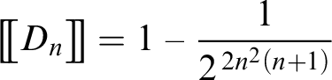 $\big [\!\big [ D_{n}\big ]\!\big ]=1-\displaystyle \frac {1}{2^{\,2n^{2}(n+1)}}$
, for any Dugundji’s formula
$\big [\!\big [ D_{n}\big ]\!\big ]=1-\displaystyle \frac {1}{2^{\,2n^{2}(n+1)}}$
, for any Dugundji’s formula
 $D_{n}$
. In particular, for every
$D_{n}$
. In particular, for every
 $n\in \mathbb {N}$
, we apply rules
$n\in \mathbb {N}$
, we apply rules
 $\Rightarrow \lor , \Rightarrow \to $
and
$\Rightarrow \lor , \Rightarrow \to $
and
![]() to decompose the formula
to decompose the formula
 $D_{n}$
into a hypersequent formed by a multiset of sequents each one of them having the following general form:
$D_{n}$
into a hypersequent formed by a multiset of sequents each one of them having the following general form:
 $$ \begin{align*}(p_{1}\to p_{1})^{n},\ldots,(p_{n+1}\to p_{n+1})^{n},p_{j}\Rightarrow p_{i},\end{align*} $$
where
 $i\neq j$
and
$i\neq j$
and
 $1\leqslant i,j\leqslant n+1$
. The number of components is
$1\leqslant i,j\leqslant n+1$
. The number of components is
 $n^{2}+n$
(we omit the component containing only boxed formulas in the antecedent, which can be removed without affecting the counting of the top-hypersequents). Since the number of implications in the antecedent of every component is
$n^{2}+n$
(we omit the component containing only boxed formulas in the antecedent, which can be removed without affecting the counting of the top-hypersequents). Since the number of implications in the antecedent of every component is
 $(n+1)\cdot n$
, the total number of implications to be analyzed in the hypersequent will be
$(n+1)\cdot n$
, the total number of implications to be analyzed in the hypersequent will be
 $(n+1)\cdot n \cdot (n^{2}+n)$
. Therefore, the number of top-hypersequents is
$(n+1)\cdot n \cdot (n^{2}+n)$
. Therefore, the number of top-hypersequents is
 $2^{(n+1)^{2}\cdot n^{2}}$
.
$2^{(n+1)^{2}\cdot n^{2}}$
.
We now need to compute the number of non-axiomatic top-sequents. Given a component:
 $$ \begin{align*}(p_{1}\to p_{1})^{n},\ldots,(p_{n+1}\to p_{n+1})^{n},p_{j}\Rightarrow p_{i},\end{align*} $$
there are
 $n(n-1)$
implications whose analysis does not lead to any axiomatic top-hypersequent, namely the implications
$n(n-1)$
implications whose analysis does not lead to any axiomatic top-hypersequent, namely the implications
 $p_{k}\to p_{k}$
, where
$p_{k}\to p_{k}$
, where
 $k\neq j,i$
. Therefore, we can conclude that the hypersequent whose analysis will lead to complementary axioms has every component of the form:
$k\neq j,i$
. Therefore, we can conclude that the hypersequent whose analysis will lead to complementary axioms has every component of the form:
 $$ \begin{align*}(p_{k_{1}}\to p_{k_{1}})^{n},\ldots,(p_{k_{n-1}}\to p_{k_{n-1}})^{n},p^{n+1}_{j}\Rightarrow p^{n+1}_{i},\end{align*} $$
where
 $\{k_{1},\ldots ,k_{n-1}\}= \{1,\ldots ,n+1\} - \{j,i\}$
. Since the components are
$\{k_{1},\ldots ,k_{n-1}\}= \{1,\ldots ,n+1\} - \{j,i\}$
. Since the components are
 $n^{2}+n$
, the number of complementary top-hypersequents is
$n^{2}+n$
, the number of complementary top-hypersequents is
 $2^{(n-1)\cdot n\cdot (n^{2}+n)}\,=2^{n^{4}-n^{2}}$
.
$2^{(n-1)\cdot n\cdot (n^{2}+n)}\,=2^{n^{4}-n^{2}}$
.
As a consequence, we can state that for every
 $n\geqslant 1$
:
$n\geqslant 1$
:
 $$ \begin{align*}\big[\!\big[ D_{n}\big]\!\big]=\displaystyle\frac{\#\mathsf{top}(D_{n})-\#\mathsf{top}^{0}(D_{n})}{\#\mathsf{top}(D_{n})}= \displaystyle\frac{2^{(n+1)^{2}\cdot n^{2}} -2^{n^{4}-n^{2}}}{2^{(n+1)^{2}\cdot n^{2} }}= 1- \displaystyle\frac{1}{2^{\,2n^{2}(n+1)}}.\end{align*} $$
□
Example 4.2.
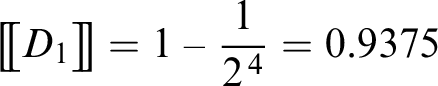 $\big [\!\big [ D_{1}\big ]\!\big ]=1-\displaystyle \frac {1}{2^{\,4}}=0.9375$
and
$\big [\!\big [ D_{1}\big ]\!\big ]=1-\displaystyle \frac {1}{2^{\,4}}=0.9375$
and
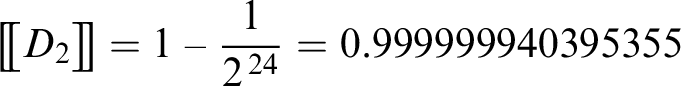 $\big [\!\big [ D_{2}\big ]\!\big ]=1- \displaystyle \frac {1}{2^{\,24}}=0.999999940395355$
.
$\big [\!\big [ D_{2}\big ]\!\big ]=1- \displaystyle \frac {1}{2^{\,24}}=0.999999940395355$
.
The next results offer yet another perspective on Dugundji’s theorem through fractional semantics.
Proposition 4.6. For any
 $m,n\in \mathbb {N}^{+}$
such that
$m,n\in \mathbb {N}^{+}$
such that
 $n < m$
, we have
$n < m$
, we have
 $0<\big [\!\big [ D_{n}\big ]\!\big ] < \big [\!\big [ D_{m}\big ]\!\big ]$
.
$0<\big [\!\big [ D_{n}\big ]\!\big ] < \big [\!\big [ D_{m}\big ]\!\big ]$
.
Proof. It suffices to observe that if
 $n < m$
, then
$n < m$
, then
 $\Big (\frac {1}{4}\Big )^{m^{3}+m^{2}}\hspace {-10pt}<\Big (\frac {1}{4}\Big )^{n^{3}+n^{2}}$
and thus
$\Big (\frac {1}{4}\Big )^{m^{3}+m^{2}}\hspace {-10pt}<\Big (\frac {1}{4}\Big )^{n^{3}+n^{2}}$
and thus
 $1-\Big (\frac {1}{4}\Big )^{n^{3}+n^{2}}\hspace {-10pt}<1-\Big (\frac {1}{4}\Big )^{m^{3}+m^{2}}$
.□
$1-\Big (\frac {1}{4}\Big )^{n^{3}+n^{2}}\hspace {-10pt}<1-\Big (\frac {1}{4}\Big )^{m^{3}+m^{2}}$
.□
Corollary 4.7. For every
 $n\in \mathbb {N}$
,
$n\in \mathbb {N}$
,
 $\mathsf {HK}$
does not prove
$\mathsf {HK}$
does not prove
 $\Rightarrow D_{n}$
.
$\Rightarrow D_{n}$
.
Proof. Straightforwardly by Proposition 4.6.□
Proposition 4.6 marks an informational refinement with respect to standard Kripkean semantics. In fact, the fractional approach allows for a fine-grained analysis of K-invalidities. In particular, the sequence of rationals
 $\big [\!\big [ D_{0}\big ]\!\big ],\big [\!\big [ D_{1}\big ]\!\big ],\ldots $
generated by the fractional evaluation of Dugundji’s formulas proves rapidly approaching near to its limit
$\big [\!\big [ D_{0}\big ]\!\big ],\big [\!\big [ D_{1}\big ]\!\big ],\ldots $
generated by the fractional evaluation of Dugundji’s formulas proves rapidly approaching near to its limit
 $1$
without ever reaching it.
$1$
without ever reaching it.
5 Concluding remarks
In this paper, we syntactically framed the basic modal logic K within the bilateral hypersequent calculus
 $\overline {\overline {\mathsf {HK}}}$
satisfying stability and invertibility of the logical rules. We showed how to use
$\overline {\overline {\mathsf {HK}}}$
satisfying stability and invertibility of the logical rules. We showed how to use
 $\overline {\overline {\mathsf {HK}}}$
in order to fractionally interpret modal formulas: any modal formula A is evaluated in terms of the ratio between axiomatic top-hypersequents and the totality of the top-hypersequents figuring in any derivation of A. Such a result has been achieved by generalizing and, then, adapting a methodology originally designed for classical propositional logic. Moreover, we argued that fractional semantics also conveys a different way of thinking about proof-theoretic semantics due to its commitment to the primacy of the notion of (analytic) proof. Here, in particular, our semantic treatment of K should be understood as a step toward a proof-theoretic semantics in modal settings (for other attempts in this direction see [Reference Leszcczyńska19, Reference Parisi23]).
$\overline {\overline {\mathsf {HK}}}$
in order to fractionally interpret modal formulas: any modal formula A is evaluated in terms of the ratio between axiomatic top-hypersequents and the totality of the top-hypersequents figuring in any derivation of A. Such a result has been achieved by generalizing and, then, adapting a methodology originally designed for classical propositional logic. Moreover, we argued that fractional semantics also conveys a different way of thinking about proof-theoretic semantics due to its commitment to the primacy of the notion of (analytic) proof. Here, in particular, our semantic treatment of K should be understood as a step toward a proof-theoretic semantics in modal settings (for other attempts in this direction see [Reference Leszcczyńska19, Reference Parisi23]).
In conclusion, we would like to hint at some themes for further research. First of all, it could be interesting to extend the fractional approach so as to include other systems of modal logic. Such an extension can be conducted along two different directions. On the one hand, one could take into account non-normal modal logics weaker than K, not characterized by Kripkean semantics, as well as stronger logics, such as
 $S4$
, serving as base of epistemic logics. On the other hand, it would be tempting to explore the relation with other proof-theoretic frameworks. We are inclined to think, in fact, that the fractional interpretation is invariant under other calculi (such as nested sequents, labeled sequents, and prefixed tableaux), as long as these fulfill the three requirements of bilateralism, invertibility and stability. Moreover, the properties of the system
$S4$
, serving as base of epistemic logics. On the other hand, it would be tempting to explore the relation with other proof-theoretic frameworks. We are inclined to think, in fact, that the fractional interpretation is invariant under other calculi (such as nested sequents, labeled sequents, and prefixed tableaux), as long as these fulfill the three requirements of bilateralism, invertibility and stability. Moreover, the properties of the system
 $\overline {\overline {\mathsf {HK}}}$
(and its possible extensions) could be also investigated from a more traditional proof-theoretic perspective by presenting a Gentzen-style cut-elimination algorithm.
$\overline {\overline {\mathsf {HK}}}$
(and its possible extensions) could be also investigated from a more traditional proof-theoretic perspective by presenting a Gentzen-style cut-elimination algorithm.
Lastly, it is worth observing that fractional semantics can be also conceived as an attempt to introduce a measure of invalidity, blurring the rigid partition between valid and invalid formulas. In this respect, our treatment could be fruitfully related to the work in [Reference Grant15] in which some semantic criteria are introduced in order to measure the inconsistency of modal formulas.
Acknowledgment
We wish to thank two anonymous referees for their useful comments which helped us to improve the overall quality of the paper.


 Open access