


1. INTRODUCTION
For several years, researchers have been assembling large databases for better knowledge and analysis of the behaviour of users, with and without driving assistance systems. Numerous experimentations have been carried out in various countries to measure the impact of such systems on speed limit compliance for example (Carsten and Tate, Reference Carsten and Tate2005; Ehrlich, Reference Ehrlich2009). Many studies refer to real-time locating systems which tell the user what the legal speed limit is at his current position (Intelligent Speed Adaptation systems). Accurate positioning is therefore of great importance for post-processing analyses.
There are many real-time algorithms to be found, both in literature and implemented on board systems, which determine a vehicle's position on the network, using multiple data sources, including a digitised map of the road system (White et al., Reference White, Bernstein and Kornhauser2000; Quddus et al., Reference Quddus, Ochieng, Zhao and Noland2007). Such algorithms use information such as vehicle's direction and speed, as well as its position at the previous instant, to provide in real time the most likely arc on which the vehicle is situated. A map-matching error may be crucial for real-time applications. An example would be when the system positions a vehicle on a deceleration lane when it is in fact on a motorway.
Real-time map-matching algorithms implemented in these systems have to perform extremely well to provide correctly geolocated information (Quddus et al., Reference Quddus, Noland and Ochieng2009). Based on the Global Positioning System (GPS), map-matching errors are not rare. This not only impairs the quality of the information provided, but also complicates the analysis of experimentation data for assessment purposes. Any such locating errors need to be detected and rectified before speed-behaviour data can be statistically analysed (Traisauskas et al., Reference Traisauskas, Juhl, Lahrmann and Jensen2007).
In this article, we propose a batch-mode algorithm to handle important databases generated by probe vehicles. This differs from classic real-time algorithms in that it is based on the Multiple Hypothesis Technique (MHT) which makes it possible to retain more than one position or path for each GPS point handled and later selects the best routes via a weighting system, at the end of the journey's processing (Pyo et al., Reference Pyo, Shin and Sung2001). Here, we propose a new weighting criterion which is no longer based on distances between GPS points and network arcs, but on the area formed between the GPS trajectory and the path. In addition, we propose to store paths in tree form, making it possible to achieve excellent performance in terms of processing speed, while retaining a large number of plausible routes.
Our aim is to determine, from the list of GPS points, the closest route to those points. Unlike with real-time algorithms, we do not retain the most “likely” arc, but a set of possible ones. The search for the “closest” path is done in a global way. It is those points situated before and after the point being processed that determine the arc to be associated with the GPS point. Let us consider the following example: the vehicle is travelling on a motorway and the position given by the GPS does not tell us whether the vehicle is on the motorway, on the deceleration lane, or even on the secondary network. Only the positions before and after the one being handled tell us exactly if the vehicle is on the motorway itself or on the slip road.
The algorithm described hereafter is essentially based on the topology of the network on which we are looking for the “closest” route to the vehicle's GPS positions. The algorithm is similar to that of Marchal et al. (Reference Marchal, Hackney and Axhausen2005), which on handling each GPS point stores in memory a limited number of paths closest to the GPS points according to a weighting system for the arcs making up the path. Our algorithm differs in the way in which it stores the data in memory. Arcs associated with GPS points are stored in tree form. Each node in the tree is associated with a topological arc, a score and possibly a GPS point. The way up a tree from its root to a leaf corresponds to a path. The set of paths forms the possible paths for the GPS points handled. Storage in tree form means we obtain excellent performance in terms of rapidity and better management of memory space. Finally, we use a system of weighting criteria which gives us excellent results that the user is free to modify to take other parameters into account, or adapt the algorithm to his own data sets and network.
In the first part of this paper, the basics of the algorithm are presented. First of all, the geometrical and topological criteria which allow a score calculation for each route are detailed. Then, the way in which routes are stored using a tree is presented. In the second part, details of the algorithm's steps are given. How points are positioned on the arcs of the route selected by the algorithm is also explained. In the third part, the algorithm is tested on two data sets. One comprises data gathered at half-second intervals on a sample during a month's journeys of a hundred or so drivers on the urban and suburban networks of Greater Paris. This data set was collected in the scope of an assessment of the LAVIA system, which adjusts vehicle speed to the legal speed limit (DSCR, 2008) when it is exceeded. The other dataset includes data collected in the Toulouse agglomeration with an experimental vehicle.
2. ALGORITHM BASIS
The map-matching algorithm is based on a determination of a system of weights with a view to selecting the closest path to the GPS points and the storage of paths.
2.1. Determination of the weighting criteria system
2.1.1. Definition and score of a path
A path corresponds to a vehicle's trajectory adjusted to the network which models the road system. A path C is defined as a series of p oriented topological arcs noted A1, A2,…Ap which verify the following condition: the terminal tip of the oriented arc Ai must correspond to the initial tip of the oriented arc Ai+1 where i < p. This definition assumes that the vehicle does not make U-turns on a traffic lane.
Let E = (P1, P2…Pn), a set of GPS points. Let C = (A1, A2…Ap), a path made up of arcs A1,A2,…Ap. A topological arc of the path is associated with each GPS point. For each association, the distance between the GPS point and the associated topological arc is calculated.
We impose the following obligations:
• point P1 must be associated with arc A1;
• if point Pi is associated with arc Aj, point Pi+1 must be associated with arc Ak with k >= j;
• point Pn must be associated with arc Ap.
The function fE,C of N →N associates the index of a GPS point with a path arc index. By construction, f is an increasing function and verifies f(1) = 1 and f(n) = p. This function makes a GPS point corresponding to a topological arc of the path. Function f is not surjective; that means, arcs of the path are not necessarily associated with GPS points.
The score S of a path associated with a function f is the sum of two weights W1 and W2.
 $$S(E,C,{\,f_{E,c}}) = {W_1}(E,C,{\,f_{E,c}}) + {W_2}(C)$$
Weight W1 is linked to the position of GPS points in relation with associated arcs, while weight W2 depends on the path's geometry. Weight W2 is independent from the GPS points of function f. It depends only on path C. It is linked to the angles formed by two consecutive topological arcs and gives priority to paths with straight and curved sections, over paths with acute angles. In the rest of the document, for a set E of GPS points, we shall try to find the minimum-score path that meets other criteria such as, for example, maximum distance between the point and its associated arc.
2.1.2. Weight W1 according to the area defined by the GPS points and the path
Weight W1 can be defined in several different ways, for example, by calculating the distances between points and their associated arcs or by calculating the area between the GPS points and the path.
Weight W1 can be defined as the sum of distances between each GPS point and its associated arc (Figure 1).
 $${W_1}(E,C,{\,f_{E,C}}) = \sum\limits_{i = 1}^n {d({A_{\,f\,(i)}}}, {P_i}) = \sum\limits_{i = 1}^n {{d_i}} $$
where di is the distance between point Pi and arc Af(i).

Figure 1. Distances between points to arcs.
In Figure 1, this weight corresponds to the sum of lengths of the segments linking each GPS point to its projection on the path. This weighting provides very good results (White et al., Reference White, Bernstein and Kornhauser2000) but it does have a weakness since it does not take into account the distance covered by the vehicle between two successive positions. Data from on board systems is generally delivered at fixed time intervals, which means that sections on which the vehicle stops or moves slowly are over-weighted. To avoid such bias, we can modify weight W1 by multiplying for example each elementary weight corresponding to the distance between the GPS point and its associated arc, by the spot speed or the distance covered between two successive positions. Multiplying the distance from point to arc by the distance covered is “roughly” the same as calculating the area between GPS points and path.
We prefer to define weight W1 as the area between GPS points and the path (Figure 2). This area is made up of elementary areas defined from points Pi, Pi+1, Hi, Hi+1 or Hi (respectively Hi+1) is the closest point of the associated arc to Pi (respectively Pi+1).
 $${W_1}(E,C,{\,f_{E,C}}) = \sum\limits_{i = 1}^{n - 1} {Area({P_i},{P_{i + 1}},{H_i}}, {H_{i + 1}})$$
with Hi the closest point of the associated arc to point Pi.

Figure 2. Areas between points to arcs.
We therefore need to calculate the elementary area of the polygon made up of points Pi, Pi+1,Hi and Hi+1. For simplicity, we made the assumption that Hi (respectively Hi+1) is the projected orthogonal of Pi (respectively of Pi+1). This is not necessarily the case since Hi is the point of the arc that is closest to Pi (projection on an arc, not on a straight line). To start with, we suppose that points Hi and Hi+1 are situated on the same segment. Two cases have to be considered:
• points Pi and Pi+1are situated on the same side of the segment and the elementary area is
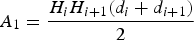
(4) $${A_1} = \displaystyle{{{H_i}{H_{i + 1}}({d_i} + {d_{i + 1}})} \over 2}$$
• points Pi and Pi+1 are situated on either side of the segment (Figure 3) and the elementary area is
(5)$${A_1} = \displaystyle{{{H_i}{H_{i + 1}}} \over 2}(\displaystyle{{d_i^2 + d_{i + 1}^2} \over {{d_i} + {d_{i + 1}}}})$$Figure 3. Polygon with Pi and Pi+1 on either side of the path.


Now we suppose that points Hi and Hi+1 are no longer situated on the same segment. The precedent formulae are extended by replacing the distance HiHi+1 by the difference between the curvilinear abscissa of point Hi+1 and that of point Hi along the path. The precedent formulae become:
 $$\left\{ {\matrix{ {{A_1} = \displaystyle{{s({H_{i + 1}}) - s({H_i})} \over 2}({d_i} + {d_{i + 1}})} \cr {{A_2} = \displaystyle{{s({H_{i + 1}}) - s({H_i})} \over 2}(\displaystyle{{d_i^2 + d_{i + 1}^2} \over {{d_i} + {d_{i + 1}}}})} \cr}} \right.$$
This way of weighting sometimes gives incorrect results, particularly when Hi and Hi+1 are the same points. In the two following examples, the precedent formulae give us an area of zero, since the two points Hi and Hi+1 are merged.
The above formulae are modified, replacing distance HiHi+1 with the maximum of the distances HiHi+1 and PiPi+1, to obtain the following pseudo-areas A′1 and A′2:
 $$\left\{ {\matrix{ {A_1^{\prime} = \displaystyle{{\max (s({H_{i + 1}}) - s({H_P{i}}),{P_{i}}{P_{i + 1}})} \over 2}({d_{i}} + {d_{i + 1}})} \cr {A_2^{\prime} = \displaystyle{{\max (s({H_{i + 1}}) - s({H_{i}}),{P_{i}}{P_{i + 1}})} \over 2}(\displaystyle{{d_i^{2} + d_{i + 1}^{2}} \over {{d_{i}} + {d_{i + 1}}}})} }} \right.$$
When Hi and Hi+1 are situated on the same segment and on the orthogonal projections of points Pi and Pi+1, we have the following relationships:
 $$\left\{ {\matrix{ {A_1^{\prime} = {{{A_1}} / {\cos (\alpha )}}} \cr {A_2^{\prime} = {A_2}/\cos (\alpha )} }} \right.$$
where α is the angle formed between segment PiPi+1 and the arc associated with the two points. We notice, therefore, those pseudo-weights A'1 and A'2 take into account the parallelism between the vehicle's GPS trajectory and the path on which the vehicle is located. Subsequently, weight W1 will be calculated with the pseudo-area formulae.
2.1.3. Weight W2 related to angles formed between two successive arcs
Taking the example of an intersection, we illustrate the relevance and importance of weight W2 linked to the angles formed between two successive arcs (Figure 4).

Figure 4. Example of a real path decision. Pi denotes the raw GPS positions, Ai the map segments, and θ(Ai,Aj) the angular weights between segments.
Let us consider two possible paths: C1 = (A1, A4, A5, A3) and C2 = (A1, A2, A3). Intuitively, points P1, P2… and P7 are located on path C2. But because of the position of points P3, P4 and P5 which are closer to arcs A4 and A5 than to arc A2, the GPS points are closer in terms of distance to path C1 than to path C2. The vehicle cannot have travelled along arcs A4 and A5 because the angle formed by these two arcs is incompatible with the vehicle's speed.
Weight W2 of a path is defined as the sum of the elementary weights linked to the angle formed between two successive arcs.
 $${W_2}(C) = \sum\limits_{i = 1}^{n - 1} {w({\theta _i}} )$$
where C = (A1,A2,…An) is a path made up of arcs A1,A2,…An and θi is the angle formed by the two successive arcs Ai and Ai+1. The angle θ is in the range [0;π]: the direction of rotation is not taken into account.
In our example, weight W2 linked to the angles formed by two consecutive arcs, penalises C1-type paths with acute angles, in favour of paths which are locally rectilinear, like path C2. The arbitrarily-chosen elementary weight w(θi) is a generalised exponential-type function which, in the range [0;π] is maximal for θ = 0 (corresponding to a U-turn) and minimal for θ = π.
 $$w(\theta ) = A{e^{ - B{{(2\theta /\pi )}^c}}}$$
Weight w(θ) depends on 3 parameters A, B and C. Parameter A determines the value of weight w when θ = 0 (w(0) = A) which corresponds to a U-Turn. Parameter B fixes the value of weight w when θ = π/2 (w(π/2) = Ae−B). Finally, parameter C is the power parameter.
The values of the angular weights are experimentally fixed, and obey different rules: in particular, when the weights are quite high that means we want to avoid these movements. For example, when the turning angle is less than π/4, we assign a big value to A. The value of parameter B is then deduced using the desired penalisation for π/2 angles. It has been chosen to authorize right angles turns, but with a small penalisation.
For angles equal or greater than 3π/4, the penalisation is very low because it corresponds to straight routes, which are favorised by the algorithm.
In Table 1, we can see that when the angle between two edges is low, the angular weight is quite high. Generally, it is not possible to change from one arc to another when the angle is less than π/4.
Table 1. Angular weights.

For angles greater than π/2, the angular weight is low and it gives an advantage to straight trajectories.
The angular weight is useful for complex intersections where it gives priority to “smoothed” trajectories. When a driver does a U-Turn at an intersection or node of the network, the angle between the two consecutive arcs is θ = 0. In Table 1, the value of the parameter A is very high. Consequently, the algorithm will give priority to paths with no U-turn.
Of course, a deeper study could be carried out to define more precisely the link between the angle and the values of the weights, through a parametric study. In our case, we have mentioned in Table 1 the most suitable parameters according to the processed data sets.
2.2. Path storage
Arcs associated with GPS points are stored in the form of a tree. Each node of the tree is associated with a topological arc and possibly a GPS point. The way up a tree from root to leaf corresponds to a path. Nodes that are not associated with GPS points correspond to arcs that are not associated with GPS points. After insertion of i GPS points (P1, P2… Pi), we have a tree Ti containing N leaves (tips of the tree). The set Si will comprise N paths corresponding to the way up a tree from its root to its N leaves. The N leaves represent the N potential arcs at point Pi. To handle the following point Pi+1, only the leaves of tree Ti are analysed to build new nodes associated with point Pi+1 which will be the leaves of tree Ti+1.
After handling of point Pi+1, the leaves of tree Ti that have no thread are destroyed “virtually”. That is, they still belong to the tree but are not considered as leaves of tree Ti+1. They may be used later to search for other paths with higher scores if the path produced by the algorithm is not suitable. Storage in tree form gives us excellent performance in terms of rapidity and enables us to manage memory space more effectively.
In the example in Figure 5, tree T4 is built from 4 GPS points (P1, P2, P3 and P4). The nodes of line L4 correspond to the leaves of the tree, which are potential arcs at point P4. By travelling through the tree from root to leaves, we obtain the 6 paths of the set S4. The nodes lined up with line Li correspond to potential arcs at point Pi. Points not belonging to a line are intermediate arcs that are not associated with GPS points. The nodes in grey correspond to old nodes, virtually destroyed and not belonging to tree T4. If the algorithm should stop after processing the first four GPS points, then the path indicated would correspond to the path with the minimum score of set S4.

Figure 5. Example of a tree.

Figure 6. Construction of leaves of tree Ti+1.

Figure 7. Map-matching errors on a service road.
3. DESCRIPTION OF THE ALGORITHM
We describe the algorithm from its initialisation, through its key stages.
3.1. Initialisation of the algorithm and construction of tree T1
Let P1 be the first GPS point of the set. The algorithm is initialised with the search for a set S1 of the oriented arcs closest to the first GPS point. To find the closest arcs, a grid-based spatial index is used. The search is limited to arcs which cross or are included in cells close to the GPS point.
A parameter D is fixed, corresponding to the maximum distance between potential arcs and the GPS point to be located on an arc. Maximum distance can be high (for instance 200 metres). This increases the number of arcs candidates for each GPS position.
Let S1={A1,A2,…,AN1} be the set of oriented arcs situated at a distance less than D and let N1 be the number of elements of T1. Tree T1 associated with point P1 is made up of a “root” node and N1 leaves. If weight W1 is related to distances, then to each leaf is attributed a score which is the distance between the GPS point of the associated arc and the leaf. If W1 is related to areas, then the score of each leaf is zero since the calculation of an elementary area requires two successive points and their projection.
3.2. Sequence of the algorithm
The algorithm proceeds by iteration. At each iteration, we add a GPS point to our set of points. Note Ei, the set of i first GPS points and Ti the tree associated with the set Ei. The leaves of tree Ti correspond to the potential arcs for point Pi. By going up the tree from the root towards the leaves, we obtain the potential paths that are closest to our points. Si is the set of paths obtained at step i after insertion of the ith point. Tree Ti+1 is built from tree Ti and more precisely from its leaves and the GPS point Pi+1.
3.2.1. Tree Ti
Let us suppose that we have handled i GPS points. At the outcome of this processing, we have a tree Ti. The leaves of tree Ti are all associated with distinct arcs which are all situated at a distance below a threshold D (maximum distance between a GPS point GPS and its associated arc) from the ith GPS point.
3.2.2. Construction of tree Ti+1
Tree Ti+1 is built from tree Ti and point Pi+1. We analyse the leaves of tree Ti associated with point Pi and from these we build the leaves of tree Ti+1.
The leaves of the tree are built in two stages. The first consists of building potential leaves for tree Ti+1, the second in deleting certain leaves in order that all arcs associated with leaves remain distinct (Figure 6).
3.2.3. Creation of leaves of Ti+1
For each leaf of Ti, we apply the following procedure. Let Lj be the leaf of the tree being processed. Let Aj be the arc associated with the leaf being handled and Nj, the termination point of Aj. Two cases are possible:
• If the distance between arc Aj and point Pi+1 is less than D, arc Aj is a potential arc at point Pi+1. We suppose here that between points Pi and Pi+1, the vehicle has not changed arcs. A new node is created, associated with arc Aj, possible leaf of tree Ti+1. A score corresponding to the score of path A1,…,Aj is attributed to this node, calculated from the score of leaf Lj.
• Now let us suppose that between points Pi and Pi+1, the vehicle has changed arcs. Via the graph associated with the network, we look for arcs situated at a distance which is less than that between points Pi and Pi+1 and point Nj. Where (Aj,k) is the set of these oriented arcs, for each of these arcs Aj,k, if this arc is situated at a distance less than D from point Pi+1, a new node is created, associated with arc Aj,k. A score is attributed to this node, corresponding to the score of path A1,…,Aj,k calculated from the score of leaf Lj. If arc Aj,k is not linked to the node via point Nj, intermediate nodes are added, associated with the intermediate arcs between Aj and Aj,k.
3.2.4. Deletion of leaves of Ti+1
Some leaves are deleted in order to keep the distinction between arcs associated with leaves. When an arc is associated with more than one node, only the node with the minimum score is retained. Thus, when two paths end with the same arc, only the path with the minimum score is retained. As all these arcs are situated at a distance less than the limit D from the GPS point Pi+1, the number of leaves of Ti, and consequently the number of potential paths, is limited. The closest path to the points of set Ei+1 corresponds to the path through the tree from root to leaf with the minimum score.
3.3. Discontinuation of the algorithm
The algorithm stops in the presence of a jump in GPS positions (d(Pi,Pi+1) > delta_d). When this happens, the map-matching algorithm has to be reinitialised from the first exploitable point found after such a jump. The algorithm also stops if the GPS signal is lost, if the acquisition time between two GPS positions is longer than the threshold time interval: delta_t.
3.4. Positioning of GPS points on the path
The algorithm ends with the positioning of GPS points on the best path. The second stage, less important, makes it possible to better locate points on the path obtained in the first stage, by considering other parameters such as speed. Let us suppose that for the set of GPS positions to be located, we have determined the topological arcs on which they are to be positioned. Positioning is carried out by iteration. Let Pi be the point GPS at time ti to be positioned on arc Ai and Pi−1, the vehicle's position at the preceding time ti−1. We suppose that this point has been located on the associated arc. Where Pmapi−1 is this position, we look for position Pmapi, the location of point Pi on arc Ai. There are two methods for positioning the vehicle on arc Ai at time ti:
• by calculating the vehicle's position from the preceding position Pmapi−1, the vehicle's speed between the two times ti−1 and ti and the geometry of the network;
• by projecting point Pi on arc Ai.
Let P1i be the point with coordinates (e1i,n1i) calculated with the first method from previous position Pmapi−1 and speed data. Let P2i be the point with coordinates (e2i,n2i), calculated with the second method, the projection of point Pi on Ai. The positioning of point Pmapi consists of estimating the position of vehicles from the two points P1i and P2i described previously.
3.4.1. In the literature
According to Quddus et al. (Reference Quddus, Ochieng, Zhao and Noland2003), the longitude and latitude coordinates of the located point Pmapi on the arc can be calculated from the two positions P1i and P2i by the following formulae:
 $$\left\{ {\matrix{ {\hat e_i^{map} = \displaystyle{{\sigma_2^2} \over {\sigma_1^2 + \sigma_2^2}} e_i^1 + \displaystyle{{\sigma_1^2} \over {\sigma_1^2 + \sigma_2^2}} e_i^2} \cr {\hat n_i^{map} = \displaystyle{{\sigma_2^2} \over {\sigma_1^2 + \sigma_2^2}} n_i^1 + \displaystyle{{\sigma_1^2} \over {\sigma_1^2 + \sigma_2^2}} n_i^2} }} \right.$$
where σ1 (respectively σ2) is the error variance on the longitude or latitude measurement of point P1 (respectively P2).
It is difficult to estimate the different effort variances described above and that is why we proceed differently in practice.
3.4.2. In practice
In practice, we use a parameter, called k here, kÎ[0;1], which corresponds to the weights of the GPS speeds data. It is very difficult to estimate the error variances mentioned above. We can for instance, fix a value for k (k=0·5), when the precision of the GPS data and of cartography is not available. We can also vary the values of k, between 0 and 1, according to the distance between the GPS point and its projection on the arc. When the GPS point is too far away from the arc, this means the point and its projection are not reliable and in this case it would be better to use data on speed rather than on localisation.
 $$k(d) = {e^{ - {{(d/\sigma )}^2}/2}}$$
where σ is the standard error of the GPS.
Using this formula, when the point is far from the arc, speed is privileged compared to the GPS position. In general, the GPS speed is far more accurate than the position. With the above parameter k, when the point is far from the arc, we can give more confidence to speed data than the projection of the point on the arc.
When the speed is low (3 ms−1 or less), the localisation thanks to GPS is less accurate and we only use the speed data. When the speed is lower than 1 ms−1 we consider that the vehicle is stopped.
We do not reason on the basis of the vehicle's 2D coordinates, but in one dimension with the curvilinear abscissa along the path calculated in the first stage of the algorithm. Let s(Pi) be the vehicle's curvilinear abscissa. We calculate the curvilinear abscissa of the location of point Pi using the following formula:
 $$s({P_i}) = k(d)s({H_i}) + (1 - k(d))(s({P_{i - 1}}) + {\Delta _{dist}}({P_{i - 1}};{P_i})$$
with Hi the projection of point Pi on the associated arc, Δdist(P i −1;P i)the distance covered by the vehicle calculated from speed data between the two positions Pi−1 and Pi, and s(Hi): the curvilinear abscissa of the projection Hi of point Pi on the associated arc.
4. ADDITIONS OF VARIABLES AND EXTRA PARAMETERS
In the algorithm described above, a path's score is made up of two terms, W1 and W2. We may add other weights in order to improve the algorithm. For example, a weight W3 related to the difference in angle between the vehicle's direction and that of the associated arc.
5. PERFORMANCE OF THE ALGORITHM
We tested the algorithm on two data sets. The first dataset was collected with a simple GPS device, the second set during a large experimentation using probe vehicles.
The road network used to locate records is based on OpenStreetMap data. This network offers some advantages: free to use, network oriented arcs and much information attached to arcs (Table 2).
To evaluate our algorithm, we implemented two algorithms to compare their results with ours. The first algorithm is an algorithm which only locates the GPS data on the nearest arc. The second algorithm is based on the Greenfeld algorithm. This algorithm uses a weighting system based on similarity criteria. This algorithm also takes into account the network connectivity. We choose this algorithm because it is relatively simple to implement and it provides quite good results (Greenfeld, Reference Greenfeld2002). For each data set and algorithm, we calculate as indicator the percentage of correct map-matching.
In order to set up a detailed ground truth and to evaluate the accuracy of position on arcs, it would have been necessary to have the exact positions of vehicles which can be delivered by Real-Time Kinematic GPS (RTK GPS) with centimetre accuracy. This sensor was not available for any of our real data sets, and we thus needed to manually assess the real route. For the first data set, the data were collected by the authors themselves, and the true route was known.
For the second data set, we analysed the 30 first journeys of the drivers by comparing the GPS traces with regard to the results of the algorithm. The previous indicator (percentage of correct map-matching) is therefore manually calculated comparing results of map-matching algorithms with known routes travelled by vehicles. For each position, we checked the network localisation of outputs of algorithms.
This indicator allows only for cross-track errors evaluation, and it is also important to evaluate the along-track error once the vehicle is positioned on the correct road. This issue relates to a different research area which focuses on post-processing the mapmatched data in order to improve along-track vehicle positioning using past and future speed and odometer data. This step can be done on a further stage in the data processing flow, using for example other algorithms based on coupling GNSS absolute positioning with dead reckoning (DR) system, such as odometer and gyroscope, that provides the vehicle's position relative to an initial position (Lahrech et al., Reference Lahrech, Boucher and Noyer2004) et (Zhao et al., Reference Zhao, Ochieng, Quddus and Noland2003).
5.1. GPS data
To assess the algorithm, we use a simple GPS device configured to deliver one GPS point and a speed per second. We carried out three GPS readings in suburban areas as well as in the city of Toulouse and its city centre where GPS localisation becomes difficult and where the road network is quite complex. We visualised GPS traces before and after map-matching in order to identify location errors (Figure 7).
For routes 1 and 2, the results of the basic algorithm are not good compared to the two other algorithms. The errors of the basic algorithm are mainly located at intersections, on parallel roads and service roads. These errors are avoided with the two other algorithms because they take into account the connectivity and the orientation of the network.
As we can see, the Greenfeld algorithm provides very good results (Table 3). For the three routes, the rate of good map-matching is greater than 95%. Our algorithm is better than the Greenfeld algorithm as hoped. The Greenfeld algorithm makes some errors when the trajectory of the vehicle is parallel to a candidate arc. The path to path algorithm can avoid these errors because it works on the whole journey and will choose the closest series of arcs to the GPS points. For some network configurations, our algorithm makes mistakes when it finds a path very close to the GPS points.
In the above example, the algorithm locates GPS points on one of the service roads. It appears very difficult to avoid such errors when the algorithm cannot distinguish between the main road and service roads since, firstly, the service road is parallel to the main road and, secondly, the unprocessed positions delivered by the GPS are too close the service road for the algorithm to be able to locate them on the main road. In this example, the Greenfeld algorithm does not make errors since at the beginning of the service road, GPS path and the main road have the same orientation.
We can easily avoid these errors by modifying the network (for example, we do not allow vehicles to be located on service roads which is easy to do) or adding weight by category of roads to give priority to main roads.
As shown in Figures 8 and 9, some typical errors of map-matching are avoided by our path to path algorithm since it is based on the multiple hypothesis technique which makes it possible to retain more than one position for each GPS point.

Figure 8. Typical errors avoided by path to path algorithm.

Figure 9. Some typical map-matching errors in a neighbourhood.
5.2. LAVIA data
LAVIA is the French project on Intelligent Speed Adaptation (ISA). During the project, 27 000 records were collected corresponding to 3 700 hours and 16 000 journeys. The LAVIA system is a data-logger which provides data every 0·48 s. In particular, it comprises a positioning system which determines the vehicle's position and the legal speed limit of the traffic lane on which the vehicle is situated. From all the gathered data (GPS, odometer and gyroscope), the system determines on which section of roadway the vehicle is travelling, projects the point on the digitized map of the system, and finally gives the recommended speed associated with that roadway section. The final data set contains only the real time results of the embedded positioning system which was known to have a high error rate. Therefore raw GPS data were not available, and we had to manually assess the ground truth for the first 30 journeys.
The algorithm described previously enables us to detect and rectify location errors of LAVIA data. We viewed the results given by our map-matching algorithm and manually calculated the percentage of map-matching errors for the LAVIA embedded positioning system, and for the proposed algorithm of map-matching. On the first 30 journeys comprising 12 868 GPS points, the positioning error rate for the LAVIA system is 5·6% against 0·6% for the map-matching algorithm. Thanks to the map-matching algorithm applied to the LAVIA data, 90% of the LAVIA system location errors were corrected.
6. SPEED OF THE ALGORITHM
Tests were carried out on a workstation equipped with a 2·8 GHz Pentium D processor and 2 GB of RAM. The algorithm was written in C++ for optimum performance. The speed of the algorithm is linear (0(n)) to the number of GPS points processed. As shown in Figure 10, for each GPS point, the algorithm works only with leaves of the tree which represent arcs candidates of the previous point. At each step, the number of leaves of the tree is limited to the number of arcs whose distance from the GPS point is lower than a threshold D (which is the maximum distance allowed between GPS point and arcs candidates). This way of working strongly improves the processing speed and that is why it is very suitable to large database processing.

Figure 10. Pseudo-code of our algorithm.
The processing speed is between 3 000 and 20 000 points per second, according to GPS data acquisition frequency and the accuracy of the map. It strongly depends on the parameter D, the maximum distance between an arc and a GPS point, which limits the number of potential arcs for each GPS position. The algorithm's excellent performance is due to the method of storing data in tree form (very convenient for large databases). In our method, while the map-matching is done globally, the search for potential arcs at point Pi is carried out locally.
7. IMPLEMENTATION AND AVAILIBILITY OF THE ALGORITHM
A program implementing the algorithm has been developed. Its source code and binary windows can be downloaded here: http://sourceforge.net/projects/mapmatching/. The program works with text and GPX files. It uses an oriented network based on OpenStreetMap (a free editable map of the world). It can be used anywhere since it uses the Geospatial Data Abstraction Library (GDAL) to convert GPS positions into a local projected coordinate system. As the source code is provided, users can modify the weight system of the algorithm.
8. CONCLUSION
In this paper we have presented a map-matching algorithm for the processing of large databases resulting from probe vehicles. The algorithm has been tested on complex networks and offers excellent performance in terms of localisation but also rapidity. Using the multiple hypothesis technique, the algorithm avoids typical errors of map-matching. By keeping candidate paths in tree form, the algorithm that searches for the closest path to the GPS positions provides very good performance in terms of speed. It is not as fast as a real-time algorithm but the speed is linear (0(n)) to the number of GPS points processed. Based on a weight system, the algorithm is quite simple to implement and the source code of an implementation is provided.
We note, however, a few map-matching errors when dealing with complex intersections and service roads. To avoid these drawbacks, the next step would be to pre-process the networks in order to identify the areas where the algorithm is likely to produce errors and give priority to given routes depending on the network analysed. For example, if the experimentation is carried out on suburban lanes, it is not necessary to focus on very limited speeds (less than 30 km/h for example).
Table 2. Description of routes.

Table 3. Algorithm performance.

ACKNOWLEDGEMENT
This research was funded by the French Ministry in charge of transport.


