


1 Introduction
Interest in using glacier fluctuations as an indicator for global climate change centres on the entire sample of tens of thousands of glaciers. Although satellite remote sensing may improve the situation in the future, very few glaciers have yet been studied in detail. Of course, these few glaciers have not been selected to be representative of all the world’s glaciers, but were investigated because of easy access and/or their direct importance for local activities.
Attempts are now being made to generalize existing ideas on the dynamics of glaciers (e.g. Oerlemans, 1994; Haeberli and Hoelzle, 1995). If individual glaciers can be characterized by a few numbers reflecting the dynamic properties (like mean slope, balance gradient, length), much larger samples of glaciers will be able to be used in climate-sensitivity studies.
Nevertheless, detailed studies of individual glaciers remain necessary, as they provide the best basis for testing simpler schemes. Also, the climatic information contained in historic glacier records has not been fully exploited. Knowledge of the future behaviour of glaciers is often important to tourism, hydropower and safety, and there is a need for models with which predictions can be attempted. Further development of computer modelling of individual valley glaciers should thus be useful.
2 Dynamic Calibration
One of the problems encountered in modelling a particular glacier is related to transient behaviour. Glacier maps simply provide observations of geometry without indicating the state of balance with respect to the current climate. Here even the definition of the current climate is not clear. One could define this as the mean state over a recent 30 year period and try to generate from the climate data a mass-balance profile B(h), i.e. specific balance as a function of altitude h, to force the glacier model. On the other hand, when mass-balance observations are available for a significant period of time, the mean observed specific balance profile could be taken as the current climate forcing.
When a reference balance profile has been defined and proper geometry of the glacier is available, a flow model can be run until a steady slate is reached and a comparison of observed and computed ice-surface elevation can be made. However, as mentioned above, this is not a good way to judge the performance of the model.
I propose to use a different approach if a record of glacier length L(t) exceeding the characteristic response time is available. First of all, it is assumed that at any time the balance profile B(h) can be described as
Here Bref (h) is the reference balance profile, independent of time t, and 4 B(t) a balance perturbation, independent of altitude h.
Now the following steps are taken:
-
(i) Determine the value of δ B that produces a steady-state glacier length equal to the first data point in the glacier length record.
-
(ii) Determine δ B (t) in such a way that a good match between simulated and observed glacier length record is obtained.
-
(iii) Compare snapshots from the model simulation with available glacier maps (and possibly a surface profile for a maximum glacier stand as estimated from trim lines).
-
(iv) rofiles exist, and repeat the calibration.

Fig. 1. Air photograph of Nigardsbreen, taken in 1947 (© Widerøe, Oslo). Trim lines from the 1748 maximum stand are clearly visible.
For glaciers with longer records, one or two maps and a dated maximum glacier stand are normally available. Step (ii) may seem difficult, but it is not in practice, as will be seen later. The most straightforward way is to use a function for δ B (t) that is a succession of simple step functions (as was done by Nye (1965)).
The simulation obtained in this way will provide the best approximation to the observed current state of a glacier. In its memory it carries the mass-balance history over a period equivalent to one or two times the response time. The procedure should lead to a good estimate of the behaviour of a glacier in the near future (for some imposed climate scenario that can be related to δ B). Such an estimate will be more reliable than one from an integration that takes a presumed steady state at the present time as initial condition.
A basic theory on inferring a mass-balance history from variations in glacier length was presented by Nye (1965).The inverse method developed in his paper is computationally efficient but involves linearization with respect to a datum state. As I consider long time-spans with larger changes in glacier geometry (a retreat of the glacier front over more than 4 km), the datum state should be adjusted many times. Instead, I have chosen to work with direct numerical integration of the non-linear equation.
Formally, we seek a mass-balance history in such a way that the rms difference σ between observed and simulated glacier length is minimized. We require that at the beginning and end of the record L obs = L sim, where δ B initial is

Fig. 2. Length variations of Nigardsbreen. Data from Østrem and others (1976), Haeberi (1985), Haeberli and Müller (1988), Haeberli and Hoelzle (1993) and Haakensen (1995).

Fig. 3. Mass-balance profile averaged over the period 1962–93 and hypsometry of the entire ice cover in the Nigardsvatn drainage basin. Data from Müller (1977), Haeberli (1985), Haeberli and Müller (1988), Elvehøy and others (1992), Haeberli and Hoelzle (1993) and Haakensen (1995).
such that Lsim represents a steady state. Next we assume that δ B (t) is a succession of step functions, where the number of values of δ B k is prescribed. Denoting this number by N, we have 2N unknowns (including the time k where δ B (t) takes the value δ B k) to be determined by a variational method. A straightforward way is to start with a good initial guess, where N is determined by the character of the curve of observed glacier length and the degree of detail required (or, rather, that appears meaningful in the light of other model uncertainties). A steepest-descent method can be applied to minimize σ with respect to the parameter vector P = [t 1, δ B 1, ___, tN, δ B N]. In that case a (very) large number of runs has to be carried out to determine the maximum of grad (P) in the parameter space. In practice it is more feasible to vary δ B k and t k for each K separately and progressively in time, starting from a good initial state of P (this is not difficult when a characteristic response time and steady-state solutions in dependence of δ B have been calculated first). So σ can be minimized easily by determination of optimal values of the pairs δ B k, (t) k] independently.
The dynamic calibration proposed here will be illustrated with a computer model for Nigardsbreen, Norway. A good result was obtained already for k = 9, i.e. nine pairs of values for δ B k, t k] were sufficient to obtain a fairly accurate match of simulated and observed front position for the period 1748–1993.
3. Nigardsbreen
Apart from all the material collected and analyzed in the series Glasiologiske Undersøkelser i Norge issued by the Norges Vassdrags og Energivcrk (NVE; Norwegian Water Resources and Energy Administration), the most complete overview of the morphology and history of Nigardsbreen is the paper by Østrem and others (1976). Nigardsbreen (Fig. 1) is an outlet glacier of Jostedalsbreen, with an area of 486 km2 the largest ice cap on the European continent. The present area of Nigardsbreen is about 48 km2. The glacier advanced very rapidly in the first half of the 18th century and reached a neoglacial maximum in AD 1748. After that,
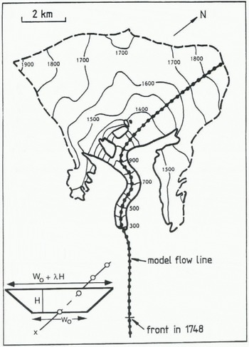
Fig. 4. Map of Nigardsbreen, based on Østrem (1988). The dotted line is the flowline as used in the numerical model. The model resolution (100 m) is three times better than the spacing of the dots.
a steady retreat took place which recently came to an end (Fig. 2). The total retreat of the snout was more than 4 km.
NVE is conducting a mass-balance programme of admirable scope on Nigardsbreen (and on many other Norwegian glaciers), and has published detailed maps of the glacier (the last one by Østrem (1988)). Mass-balance observations have been carried out since 1962. In this paper, data are used for the period 1962–93. The balance profile averaged over this period is shown in Figure 3, together with the 1988 hypsometry. The mass-balance profile of Figure 3 is taken as reference (B ref (h); see Equation (1)).
4. The ICE-Flow Model
The model is based on the one used in an earlier paper (Oerlemans, 1986). The major changes concern the resolution (changed from 300 m to 100 m grid-point spacing), slightly different flow parameters and slightly different input geometry (as a result of the dynamic calibration).
The downward flow of ice is calculated along a flowline (x axis), as indicated in Figure 4. The choice of the flowline in the upper part is rather ambiguous, but not critical to what happens at the glacier snout. It is important, however, to have the correct area–elevation distribution.
The model is of the vertically integrated type, in which simple shearing flow and sliding is considered. The vertical mean ice velocity U is entirely determined by the local “driving stress” т, being proportional to the ice thickness H and surface slope δh/δx (h is surface elevation). The lateral geometry is parameterized by a trapezoidal cross-section, having two degrees of freedom (see Fig. 4). Shape factors (e.g. Paterson, 1994) are not used.
The model equations are x is the coordinate along the flowline; x = 0 at the top): Conservation of ice volume:

glacier width at the surface:
area of glacier cross-section:
mean ice velocity in cross-section: U = U d + U s

“driving stress”:

surface elevation:
S is the area of the cross-section, and b the bed elevation.
The description of the ice velocity follows Budd and others (1979). In this approach the effect of basal water on sliding is not modelled explicitly: the bulk effect is absorbed in the sliding parameter f s. The values suggested by Budd and others (f d = 1.9 X 10⁻²⁴ Pa–3 s–1, and f s = 5.7 X 10⁻²⁰ Pa–3 m–2 s–1) are taken as a starting-point. The prognostic equation for H follows from substituting Equations (3) and (4) into Equation (2):

With the aid of Equation (6) the ice velocity can be expressed in thickness and surface slope:

Where
Substitution into Equation (8) now shows that the change of ice thickness is governed by a non-linear diffusion equation:

where the diffusivity is:

Equation (10) is solved on a 100 m grid. Time integration is done with a forward explicit scheme, which is stable if the time step is Sufficiently small. Tests have been done on grids with spacing of 300, 200, 100 and 50 m, and with a variety of time steps to ensure that truncation errors in (he difference scheme are negligibly small. A 100 m grid with a time step of 0.01 years appears to be very suitable and compatible with the accuracy of the geometric input. The flowline has 180 grid points. With the flowline as defined in Figure 4, the maximum glacier length (in 1748) was 14.3 km. The numerical model was coded in Fortran-77, and a 1000 year simulation takes about 10 min on a Macintosh Power PC 7100-66.
Geometric input was taken from the topographic map (Østrem, 1988) and a variety of other sources (Østrem and others, 1976; personal communication from O. Liestøl, 1983). Bed topography for the lower part of Nigardsbreen was taken from cross-profiles investigated through hot water drilling. In the lower valley not covered by ice it is simply taken from the map. In the accumulation basin, bed topography

Fig. 5. Simulation of the historic front variations obtained by adjusting the mass-balance perturbation δ B(t) for the period 1600–1961 (for 1962–93 the observed values are imposed).
was taken as in Oerlemans (1986), which was essentially based on the assumption of perfect plasticity (Paterson, 1994). In the literature, the characteristic yield stress has often been taken as 1 bar. However, for glaciers with a large mass turnover like Nigardsbreen, a larger value should he used (e.g. Haeberli and Hoelzle, 1995). Here we have used slope x ice thickness = constant = 15 m, corresponding to a yield stress of about 1.4 bar.
The basal topography of Nigardsbreen is not well known. However, only minor adjustments of the bed topography relative to the data used in Oerlemans (1986) were needed to get a good simulation of the historic record together with an accurate match of the 1988 profile. One may argue that the use of different flow parameters would, through the calibration procedure, lead to a significantly different bed topography. Indeed, for any set of flow parameters the bed topography can be adjusted so that a very good match between observed and calculated surface elevation for the 1988 stand can be obtained. However, as discussed in more detail later, it then becomes impossible to produce the correct record of glacier length in recent decades. So, summarizing, the constraints available for the present study cannot be met for a bed topography that deviates significantly from the one derived here.
5. Simulation of the Historic Record
Simulation of the historic record was achieved by reconstructing a mass-balance history δ B(t) for the period 1600–1961, and using the measured balance values for the period 1962–93 (the mean in this period is 0 by definition; see section 2). δ B represents a perturbation to the fit of the mean observed balance profile (1962–93). When imposed on the model it implies a change independent of elevation. For δB = –0.5 m a–1 the mean specific balance would be zero for the present-day glacier geometry. In the historic simulation, the reconstructed δB(t) cannot be directly related to the mean balance at a specific time (because the balance profiles work out differently for different glacier geometries).
As a first step, δB was chosen such that the 1710 glacier stand (L = 12.55 km) represents a steady state. This is an arbitrary way to start, but a meaningful alternative does not exist. The resulting value of δB is +0.28 m a–1. Then it appeared impossible to simulate the extremely rapid advance during the period 1710–48. A 10-fold increase in the sliding parameter f s for a few decades does the job. It results in a very fast advance of the snout, but at the same time the glacier thins so dramatically that a very strong retreat after 1750, much faster than seen in the record, is inevitable. So this option of simulating the advance was rejected. When a value of 1 m af –1 is taken as the upper limit for δB during a period of several decades, the correct 1748 stand can be simulated for δB = 1 m a–1 for the period 1670–1711, and δB = 0.34 m a–1 for the period 1711–60 (see Fig. 5). The simulated rate of advance during the period 1710–48 is about half the “observed” value. Maybe the conclusion should be that the advance rate suggested in a document by Foss (cf. Østrem and others, 1976) is inaccurate. In any case, the timing and stand of the 1748 maximum is not discussed, and the reconstruction of δB should be such that this is well simulated by the flow model. It is not difficult to match the observed length record after 1748, as demonstrated in Figure 5. This result was obtained after the calibration, in which the bed geometry was slightly adjusted to give the correct hypsometry for 1988 and to give a surface elevation very close to the measured elevations. For the part between x = 5 and x = 10 km, the rms difference after the calibration is only 5.4 m. In principle this could be further reduced by repeating the calibration procedure, but this was not considered worthwhile in view of other uncertainties (see also section 6).
The required changes in the specific balance are of reasonable magnitude. According to calculations with a mass-balance model (Oerlemans, 1992), a uniform ± 1 K temperature change would change the mean specific balance by about ± 0.9 m a–1. With this value the reconstructed balance history can be converted to temperature perturbations.

Fig. 6. Simulated glacier length until 2100, with mass balance after1993 equal to the 1962–93 mean (reference). Also shown are results from experiments in which δB(t) was perturbed in the period 1800–50 as labeled on the curves (in m a–1).

Fig. 7. Modelled response of Nigardsbreen to a slepwise change in mass balance as labelled on the curves. Times given are e-folding response times for length and volume.
Taking the period 1900–93 as a reference, it turns out that, to explain the retreat of Nigardsbreen, mean temperature in the 18th and 19th centuries should have been 0.53 and 0.27 K lower. This finding is in line with current ideas on the “Little Ice Age” (e.g. Bradley and Jones, 1995).
Concerning changes in volume, Østrem and others (1976) estimated a loss of 1.96 km3 of ice for the period 1748–1974. According to the calibrated model simulation this would be 1.63 km3 of ice. The reason for the difference is unclear, but in their paper Østrem and others state that their value is only a crude estimate.
In Figure 6 the same simulation is shown, but now running until 2100. The value for δB after 1993 is set equal to the 1962–93 average. The model predicts an advance of about 800 m relative to the present position of the snout. It would

Fig. 8. Glacier profile along the flowline, with driving stress (upper panel). The lower panel shows total velocity, sliding velocity and deformational velocity.
take 50 years to come close to this steady state. The stability of the δB(t) curve found against length variations has been studied by imposing additional mass-balance perturbations in the past. The results of this are also shown in Figure 6. Glacier length is shown for runs in which the mass balance in the period AD 1800 –50 was perturbed with a constant value (–0.4, –0.2, +0.2, +0.4 m a–1). Apparently, it takes about 100 years for the perturbation to damp out. It can also be concluded that the reconstructed mass-balance history δB(t) is well defined: small changes in δB(t) lead to a simulated glacier length record that is way off.
It can be seen in Figure 5 that a significant phase shut occurs between glacier volume and length. Typically, volume leads glacier length by 20 –40 years. Response times of Nigardsbreen have been investigated further by imposing stepwise forcing in the mass balance to a modelled glacier state in equilibrium. A few characteristic results are summarized in Figure 7, for mass-balance perturbations of +0.4 and –0.4 ma–1.
Here response time is related to an instantaneous change of the climatic state from C 1 to C 2 imposed to a glacier in equilibrium with C 1. The corresponding equilibrium glacier volumes are V 1 and V 2. The response time t rv now is the time a glacier needs to attain a volume V 2 – (V 2 – V 1/e. Similarly, the response time for glacier length (t rL) is defined. Values for t rL are indicated in the figure. Apparently, the response in volume is faster than in glacier length, in agreement with the impression from Figure 5.
Jóhannesson and others (1989) have argued that a volume time-scale can be defined as H */– B term, where H * is a characteristic ice thickness and B term the specific balance on the glacier snout. With B term = – 10 m a–1 and H * = 85 m (estimated mean value of ice thickness over the entire glacier), this yields a time-scale of only 8.5 a. It is probably more appropriate to take for H * the mean value of ice thickness over the tongue (about 130 m), or the maximum ice thickness on the tongue (about 180 m). This would yield response times of 13 and 18 a, still significantly smaller than the characteristic value of 40 a found from the present numerical model. The difference is probably related to the fact that the height–mass-balance feedback, not taken into account in the estimate ofjóhannesson and others (1989), is quite significant for Nigardsbreen, as the tongue is on a bed with a small slope. This feedback makes the response time longer.
6 Diagnosis of the Simulated 1988 and 1748 Stands
We now take a closer look at two snapshots (1748 and 1988) from the calibrated simulation. Figure 8 shows glacier profile, driving stress, total velocity and sliding velocity as simulated for 1988. It should be emphasized that the glacier is not in a steady stale. The profile of the tongue is very close to the observations (Østrem, 1988), which is of course the result of the tuning procedure. It should be added that the flow parameters suggested by Budd and others (1979) were not modified, as this brings no improvement (see section 7).
On the glacier tongue (x > 5 km) the driving stress is relatively large, typically 1,5ȓ2 bar. It drops off rapidly when approaching the snout. Sliding speed is typically two-thirds of the total speed, and peaks when ice thickness is small (this is evident from Equation (4), i.e. in the upper reaches,

Fig. 9. A comparison of simulated and “observed” glacier elevation for the maximum stand in 1748. Observed values have been inferred from trim lines by (Østrem and others (1976).

Fig. 10. The effect of changing flow parameters (f’s) on the steady-state profile for δB= 0.
in the icefall at x = 5 km and close to the snout. Although some velocity measurements have been carried out on Nigardsbreen (Østrem and others, 1976), it is difficult to use these for model validation. The measurements do not allow a calculation of the mass flux through a cross-section averaged over several years, which is the quantity that the model actually calculates.
In Figure 9 the simulated maximum stand is compared to the profile as inferred from the trim lines and terminal moraine. It appears that the simulated profile has a slightly larger elevation than the trim lines. However, there is a considerable uncertainty in deriving a mean glacier profile from trim lines. First of all, a glacier cross-profile is not level but generally shows variations of order 10 m. In general, the mean elevation in a profile will be larger than the elevation at the valley walls. On the other hand, the trim lines show maximum stands at any moment, and in theory it is possible that maximum stands were reached at different times along the profile. Given these considerations, the agreement between calculated and inferred surface elevation is good, and further fine tuning of the model simulation is not useful.
The 1988 stand as shown in Figure 9 does not represent a steady state. It appears that a steady state with exactly the same glacier length as in the time-dependent simulation for 1988 is obtained with δB = 0.08 m a–1. The calculated steady-state volume is 3.98 km3; the volume for the 1988 stand is 3.80 km3. This difference can be related to the negative balance in the period 1965–88 (in 1989 a period of

Fig. 11. Close-up of the calibrated simulation with flow parameters increased by 50%.
strong positive balance started). Anyway, the difference is small, and in 1988 the glacier was close to a steady state.
7 Changing Flow Parameters
As mentioned earlier, values for the flow parameters were taken from Budd and others (1979). It is not obvious a priori that these are the best values for Nigardsbreen. A large number of experiments were carried out to assess the effect of changing flow parameters. Because the tongue of Nigardsbreen is on a bed with a very small slope, the height—mass-balance feedback is important, and one might expect that different flow parameters (directly, affecting the glacier’s thickness) would lead to significantly different steady states (for a given mass-balance profile i>B(h)). This turns out to be the case. Figure 10 shows steady-state profiles (in case δB = 0) for Budd and others’ values of the flow parameters (dashed) and for cases in which these values were doubled and halved. Experimentation with other bed profiles shows that the large sensitivity is indeed related to the very small slope for x > 10 km. This cannot be considered a general feature of valley glaciers.
With halved and doubled flow parameters, values of δB can be found that yield the same equilibrium glacier length, of course. The shape of the snout is then only slightly different (about 15 m in ice thickness), This implies that comparing observed with simulated ice thickness is not a very powerful method of determining the flow parameters.
The next question concerns the sensitivity of the time-dependent simulations to the choice of flow parameters. For instance, if the flow parameters are increased by 50%, only small adjustments in δB(t) are needed to produce again a correct simulation of the historic record. However, it appears that the current behaviour of the glacier (advance) is not in agreement with the simulation (retreat) (see Fig. 11). The difference with the reference run is a consequence of the decreased response time: with increased flow parameters the response time decreases, and the glacier snout reacts to the negative balance for the period 1965–80. In the model, this causes a minimum glacier stand around the year 2000.
Although not in a very definite way, these experiments suggest that the flow parameters proposed by Budd and others (1979) do perform best. Therefore, these are used in subsequent numerical experiments.
8 The Next Century: Retreat Again?
In this section we investigate how Nigardsbreen would react to imposed greenhouse warming. First of all, only uniform changes in air temperature and precipitation are considered. As mentioned earlier, energy-balance modelling suggests that a 1 K warming produces a –0.9 m a–1 change in
Table 1. The imposed climate-change scenarios imposed to the glacier model. The last two columns give model output. The relative volume (last column) is with respect to AD 1950

mean specific balance (Oerlemans, 1992). Although this is a number averaged for the present glacier geometry, it is used to estimate dB/dT as 0.9 m a–1 K–1. Similarly, the effect of changing precipitation dB/dP is estimated to be 0.035 m a–1 % –1. So for a given change in temperature and precipitation the balance profile imposed on the flow model is:
where δT is in K and δP in %.
Four scenarios were considered, as shown in Table 1. The mass-balance perturbations associated with the warming rates are relative to the period 1962–93, so the warming rates should be interpreted as relative to the 1962–93 value. This is not a trivial approach, as the mean balance for 1962–93 does

Fig. 12. Glacier length and volume as calculated for four climatic-change scenarios. Runs with increasing precipitation are labelled d P
not necessarily constitute the correct reference. For each warming rate an additional run was done with an increase in precipitation, taken as +10% per degree warming.
Figure 12 shows calculated glacier length and volume for the four cases. The case “no change” corresponds to keeping the balance equal to the 1962–93 mean. It is obvious that the retreat is dramatic, even for the case of small warming rate and increased precipitation. It should be noted that when glacier length drops below 4 or 5 km the results of the model will become less accurate, because in reality the glacier would split up into several small glaciers (see Fig. 4).
Also, changes in volume are quite large. In the case of a warming rate of 0.02 K a–1 and no increase in precipitation, the ice volume remaining in AD 2100 would be only 10% of the 1950 value.
From these experiments it is also clear that Nigardsbreen (and Jostedalsbreen) could not survive in a climate just a few degrees warmer than the present one. The present calculations support the view that glaciers were absent from western Norway during the hypsithermal (Nesje and Dahl, 1993). This is of course due to the characteristic topography; the high areas carrying ice caps are relatively flat, and surface elevations are only a few hundred metres above the current equilibrium line.
Concluding Remark
Reconstructing a mass-balance history that produces the observed glacier length record of Nigardsbreen is not difficult. Although not yet fully explored, the procedure proposed in this paper to calibrate glacier models may be a good basis for projections of future behaviour. For individual glaciers the available data vary in character, quality and detail, and a uniform recipe cannot be given. In fact, for Nigardsbreen the situation is fortunate because a long record of glacier length can be combined with very good mass-balance observations. Nevertheless, in my view observed length variations provide a useful constraint in the modelling of any glacier.
Acknowledgements
Several colleagues at the Institute for Marine and Atmospheric Research are thanked for suggestions and comments on an earlier draft, notably Z. Zuo, R. van de Wal and W. Greuell. I am also grateful to R. Hindmarsh and A. Stroeven for useful comments and suggestions.


