Introduction

A knowledge of the velocity of propagation of radio waves in ice and firn is essential to the interpretation of radio-echo soundings of ice masses. Accurate determination of these velocities, either by direct measurement in the field or by measurements of permittivity in the laboratory is difficult. The problem has been discussed in several papers (e.g. Reference Bogorodskiy and FedorovBogorodskiy and Fedorov, 1967; Reference RobinRobin and others, 1969; Reference Jiracek, Bentley and CraryJiracek and Bentley, 1971). In general, field studies have been concerned with measurement of the mean velocity throughout considerable thicknesses of ice. We have to look to laboratory and theoretical studies for evidence of the effects of temperature, density, and crystal fabric on the velocity of propagation of radio waves. In this paper we report on a new technique which should help to improve the accuracy of our measurements of velocity as a function of depth. The method should help us to relate bore-hole studies of density, ice fabric, and temperature to the velocity of radio waves in ice and firn. Reference BentleyBentley (1972) has already shown the value of such information on seismic P-wave velocities, especially in relation to ice fabric. There is an obvious need for similar information in relation to radio-wave propagation.

The opportunity to develop this technique arose when planning a programme of field work on the ice cap on Devon Island in cooperation with the Canadian Continental Shelf Project. When Dr Paterson mentioned the availability of his bore holes to our radio-echo group, several possible methods of measuring absorption and velocity of radio waves were considered. Of these, the use of an interferometric technique to determine radio-wave velocities with greater precision than in former studies appeared to be both practicable and useful.

Equipment and method

The principle of the technique is to lower down a bore hole an antenna which radiates a continuous signal at a fixed frequency, to pick up the signal from this antenna after it has passed through the ice and firn to a second antenna on the surface, then to mix the received signal with the original fixed frequency to generate “beats” as the antenna is lowered. Then by measuring the spacing between successive null points we can determine the velocity of propagation by multiplying wavelength by frequency.

Fig. 1. Schematic diagram of bare-hole experiment

In practice we used a 440 MHz pulsed radio-echo system developed for general sounding purposes by M. R. Gorman. A tuneable signal at a frequency of about 440 MHz was generated by a continuous oscillator fed to a power amplifier which was switched on for about 0.5 μs to provide power to the antenna. Connection to the antenna was via low-loss co-axial cable 280 m in length, so that it was possible to lower the antenna to the maximum depth available in the bore hole on Devon Island. The receiving antenna, which consisted of a broad-band dipole in a reflector, was placed in a pit dug into the snow which was about 1.5 m deep, 1.5 m square, and placed from 4 to 41 m from the bore hole. The bore-hole antenna was designed by S. Evans with impedance characteristics to match the surrounding medium and so produce an effective radiation pattern. On the advice of P. Gudmandsen an extra choke was fitted to prevent energy running along the outer of the coaxial feed cable. The receiver itself consisted of a r.f. amplifier and a mixer to generate an i.f. signal at 60 MHz. This signal was then amplified and recorded in the standard SPRI Mark IV system, using both A-scope and intensity-modulated presentation.

Since a short pulse cannot be fully monochromatic, instead of complete fading there was a variation of the amount of fading with time throughout the pulse. As seen in FFigure 2, this produced no difficulty in interpreting the pattern of fading with depth of the antenna.

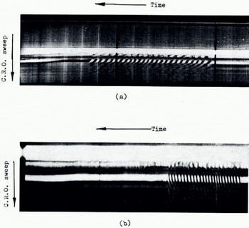
Fig. 2. Interference pattern recorded by an intensity-modulated display as the antenna is mooed in the bore hole. The broad white band is formed by direct breakthrough from transmitter to receiver during transmission. The band showing the interference pattern shows the pulse that has travelled though ice and firn. Variations of the latter band on the left of the record are due to fine adjustments of antenna depth so that measurements are made at a null point

(a) During lowering an 20 June 1973. Black marks across the film and digital information are printed every minute.

(b) During raising on 19 June 1973. This is enlarged to about three times the scale of (a) as raising by power was more rapid than lowering on a brake drum.

Identification and counting of the null points passed as the antenna was lowered and raised were done by the operator, who watched the rise and fall of the pulse on an A-scope display as the antenna was moved. When a specific point, say one half cycle after the start of the pulse, fell to zero, this was taken as the reference null point. The antenna was winched up or down in 10 m steps and a fine adjustment was made each time to stop the antenna at a null point as defined previously. The operator visually counted the number of null points each time the antenna was raised or lowered. At the same time the intensity-modulated display of the SPR1 Mark IV system recorded the changing pattern as the antenna was moved (Fig. 2). This provided a permanent record from which the number of null points passed on each 10 m move could be counted subsequently. Depths to the antenna were measured by reference to tape marks on the cable.

It was estimated by the operator that he could identify the null point to an accuracy of about ^3 cm in vertical movement of the antenna, so the error in determining the mean velocity over each 10 m interval should not exceed ±1.0 m/μs. The accuracy of the measurements is discussed later in more detail.

Since the receiving antenna was offset by a distance L from the top of the bore hole, the separation between the two antennae is (D²+L²)½ where D is the depth of the transmitting antenna. We assume straight-line propagation, which according to computations reported by Clough (see discussion, p. 159) introduces no significant errors. The change in value of (D²+L²)½ for each change of antenna depth was then divided by the number of null points to determine the wavelength at that depth.

The frequency, which is also required in order to determine velocity, was determined by a similar system of null counting in air. The separation between the transmitter and receiver was increased by carrying one antenna away from the other until the operator counted 50 null points. After fine adjustment, the distance was measured by steel tape. A system of repeated measurements eliminated errors. Use of an accurate frequency meter, or of a crystal-controlled oscillator, would save time in future. It was, however, useful in our tests to use difference frequencies, which ranged from 411.3 to 435.5 MHz.

Results

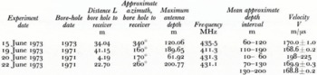
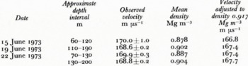
After preliminary trials on 13 and 14 June 1973, during which techniques were tried and modified, useful results were obtained on the four days when work in the bore holes was possible. The results are summarized in Table I and shown in more detail for individual 10 m intervals in Figure 3.

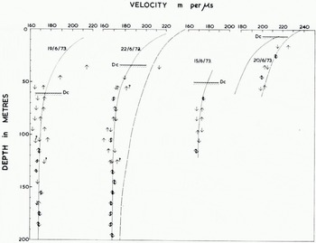
Fig. 3. Variation of velocity of radio waves with depth in the ice cap of Devon Island. Each arrow shows the mean velocity over the approximate so m interval (e.g. c. 60 to c. 70 m) in which it is shown. The. direction of the arrowhead indicates whether the measurement was taken during lowering or raising of the antenna.

The continuous line shows velocities derived from density values on the basis of Equation (1). The dashed tines show similar velocity-depth curves for Site 2 in north-west Greenland derived by Fedorov (1969). D_e indicates the critical depth above which measurement of null points is unsatisfactory

The presentation in Figure 3 also serves to indicate the reliability of the results, since the mean velocity over each 10 m interval is plotted separately for measurements made during lowering and raising of the bore-hole antenna. Below 130 m depth there is no uncertainty over the number of null points traversed, and the difference between velocities measured during lowering and raising of the antenna is consistent with our earlier discussion of accuracy. At these depths, an apparent slow cyclic variation of velocity with depth appears during both raising and lowering of the antenna. However, this variation was different in phase between runs on ig June 1973 and 22 June 1973 which were made in the same bore hole. Differences between these runs included changed values of the separation L, use of a different frequency, and changed azimuth. It is likely that one or more of these factors have affected the consistency with which null points are identified—and hence the derived velocities. It seems less probable that the small cyclic changes of velocity are due to differences of density or ice fabric between the two runs, both of which used the same bore hole but a different azimuth. We have therefore taken the mean velocity over one complete “cycle” of these variations to obtain the values given in Table I.

Table 1. Bore-hole measurements of velocity of radio waves in ice, devon island, 1973

The scatter of points in Figure 3, especially between raising and lowering of the antenna above the 130 m level, reflects uncertainty arising from the difficulty of identifying and counting null points. The pulse lost its consistent shape rapidly when the antenna was raised above a critical depth D_c — L cot φ, where φ is the critical angle for total reflection, i.e. φ = are sin C/V_d , where C is the velocity of radio waves in air and V _d the velocity in ice at the depth D_c. This difficulty over pulse shape was present both with the receiving antenna in a pit, and with the receiving antenna above the surface. It is clear that near the critical angle, significant amounts of energy reach the receiving antenna by different paths, hence destroying the steady shape of the pulse and making measurement of null points impracticable.

Discussion

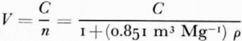
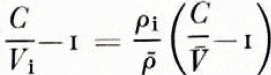
In Figure 3 we show by a continuous curve, values of velocity against depth which have been calculated from mean depth-density data made available by W. S. B. Paterson (private communication) using a linear relationship between refractive index n and density p as in Robin and others (1969. p. 461). The velocity V given by

(1)

An earlier estimate of the form of the velocity-depth curve by Fedorov (1969, p. 228) based on the density depth values for Site 2 in Greenland (Reference Anderson, Benson and KingeryAnderson and Benson, 1963, p. 396) is also shown by a dashed line. Although the densities used by Fedorov are appreciably lower than those in Devon Island up to a depth of 130 m where the two densities are equal, the major difference between the curves is due to differences in the relationship between density and velocity used in the two cases. It is clear that Equation (1) provides the better fit to the observed velocities below 60 m, although above 60 m Fedorov’s curve fits the velocities observed on 20 June 1973. However, over the depth range 50-60 m, there is a discrepancy of about 10% between the velocities as measured by us on 19 and 22 June and our measurement of 20 June. This casts some doubt on our values at shallower depth, which were made with the receiving antenna only 4 m from the top of the bore hole.

When considering our results, we must remember that, in addition to experimental factors, the value of permittivity and hence velocity varies with the shape of inhomogeneities in the firn mass. This has been discussed by Reference EvansEvans (1965), Reference Bogorodskiy, Bogorodskiy, Trepov, Fedorov and GudmandsenBogorodskiy and Fedorov (1967), Jiracek and Bentley (1971) and others on the basis of a shape factor, or “Formzahl”, proposed by Reference WienerWiener (1910). The firn near the bore hole on Devon Island had a high frequency of approximately horizontal ice layers and lenses up to at least 10 cm in thickness. Use of a vertical dipole means that the electric field will be normal to the layering, which corresponds to a low value of the Formzahl, hence a low value of permittivity and a high value for velocity. Whatever the reason for the relatively high values observed at shallower depths on 20 June 1973, it is clear that we cannot yet relate velocity to density with any high precision.

The only other technique for measuring the variation of velocity with depth in the firn zone of a polar ice sheet is that reported by Reference Clough and BentleyClough and Bentley (1970), Jiracek and Bentley (1971), and Bogorodskiy and others (1970). Velocities are found by plotting the square of the echo time from discrete reflecting layers against the square of the distance from transmitter to receiver. The results give a mean velocity to the depth of the reflecting layer, and in general this shows an increasing velocity with depth. On the plateau of east Antarctica, Clough and Bentley (1970) conclude that their results are consistent with the velocity-density relationship given in Equation (1).

As the density of firn approaches that of pure ice, variations of Formzahl become smaller. In order to extrapolate our results to greater depths, and to produce a value for comparison with results of other experiments, we have extrapolated the measured values in Table I to the velocity V_i for ice of density p_i = 0.917 Mg m^-3 by use of the relationship derived from Equation ( 1 ):

(2)

where V is the mean velocity over the depth interval for which the mean density is ρ Values of V_i are shown in Table II. The possible errors are increased over those shown in Table I due to uncertainties in the value of density, which has been extrapolated below 120 m at which level 0 = 0.899 Mg Mg.m^-3. Our best experimental measurements are those from 22 June below 130 m which give a value V_i = 167.7 ±0.3 m/μs, while other data from shallower depths indicate a similar velocity.

Table 2. Velocity of radio waves in ice of density 0.917 mg/m³ and mean temperature — 20° C

Jiracek and Bentley (1971) obtained a particularly useful result from wide-angle measurements in an ablation zone on Skelton Glacier, for which the estimated mean density was 0.907 Mg m^-3 and the velocity was 168.5±1.0 m/μs. In summarizing their results, they conclude that their best estimate of the value of the relative permittivity of pure ice, on the basis of their field observations, is 3.21 which corresponds to V_i = 167.4 m/μs. When account is taken of Wiener’s Formzahl, they believe that most observed velocities fall within his predictions using these values, but they remark that further glaciological and in situ measurements are needed.

In FFigure 4 we make a wider comparison of our field measurement of velocity with results of other workers. The laboratory data is taken from Robin and others (1969). Additional field results obtained by comparing radio-echo reflection times with ice depths observed by direct drilling or by seismic sounding are shown by circles. In general, the accuracy of these derived velocities are no better than ±.1.0 m/μs. These results are consistent with the other values.

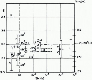
Fig. 4. Comparison of field measuremenls of the velocity of radio waves in polar ice sheets with laboratory measurements of relative permittivity of ice samples of density 0.90 Mg m^-3. Values to the left of the dashed line are laboratory measurements at lower frequencies.

Field measurements:

R. Robin, c. —20° C, bore-hale measurements.

J. & B. Jiracek and Bentley, Skelton Glacier, wide angle sounding.

(1) to (5) are derived from comparisons of radio echo soundings with bore-hole depths, (1) and (z), or with seismic soundings, (3) to (5), in the same vicinity. (1) Camp Century, (2) New ’“Byrd” station, (3) South Pole, (4) and (5) inland from Mirny and Molodezhnaya.

Laboratory measurements;

Reference KuroiwaK. Kuroiwa ([1956]) — 1 to — 15° C.

Reference Auty and ColeA. Auty and Cole (1952) —11°C.

P. Paren (private communication in 1968).

Out of six different natural-ice specimens, all having similar temperature coefficients, the two extreme examples are shown here (upper, from TUTO tunnel; lower, from 480 m depth in central Greenland).

Pi. Reference Fitzgerald and ParenFitzgerald and Paren ( 1975, p. 43) sample refrozen from deep polar ice.

P2. Fitzgerald and Paren (1975, p. 42) deep sample from “Byrd” station core.

W. Westphal (private, communication, 1963} (TUTO tunnel sample).

Reference Von HippelV. Von Hippel (1954), — 12° C.

Reference CummingC. Cumming (1952), —18° C.

Reference Lamb and TurneyL. Lamb and Turney (1949), 0 to - 190° C.

The situation shown in Figure 4 appears similar to that in relation to the velocity of seismic waves in snow and ice some 15 years ago. The considerable scatter of early measurements is gradually giving way to a consistent pattern of experimental results. Part of the scatter of the field results can now be explained by variations of the depth-density relationship for firn and ice in different localities, but other factors may also prove to be significant. Thus, the value of our experiment lies not only in the immediate results: it also shows that the technique of radio interferometry can be used for more accurate velocity determinations than other methods. Although the results above 50 m depth are questionable, at greater depths we can now achieve the accuracy necessary to study the effect of temperatures and crystal orientation on the velocity of radio waves. It is hoped that this technique will be used in other bore holes in polar ice sheets.