


Introduction
Even in the cold environments of Antarctica, surface melting can take place locally during summer. One example of this is the South Shetland Islands where drainage systems associated with snowmelt have been studied by Reference Birnie and GordonBirnie and Gordon (1980). Further, in the dry valleys, summer melting of snow and glaciers and the characteristics of permanently ice-covered lakes are reported by Reference Chinn, Green and FriedmannChinn (1993). Additionally, melting occurs locally close to nunataks in many areas due to strong absorption of solar radiation at surfaces with low albedo. However, the meltwater drainage channels and meltwater accumulation basins (hereafter called frozen lakes) described in this paper are located on the land ice mass in Dronning Maud Laud, tens of kilometres away from the closest nunatak and about 130km from the ice-shelf barrier. The features are created by snowmelt in a north-sloping area which is favourably exposed to incoming solar radiation Fig. (1). In addition, katabatic winds provide very low winter snow accumulation.

Fig. 1. Location and surface topography of the NARE 1993-94 study area in Futulgryta, Dronning Maud Land. Temperature profiles and stratigraphy from typical locations in blue ice and snow are shown. While some surface melting takes place in this area, the main melt activity seems to take place sub-surface in blue-ice fields due to the “solid-state-greenhouse effect”. Typically, the upper 5–10cm of the blue-ice fields remain frozen while the sub-surface melt layer is about 0.5 m thick. The frozen lake shown (lake Jutulsjøen) is fed by meltwater that flows into an unfrozen layer that lies between the underlying main ice body of the frozen lake and the top ice cover. This means that the “solid-state-greenhouse effect” is present at the frozen lake as well. The top ice cover of lake Jutulsjøen was typically 10–20 cm thick, whereas the underlying layer of waler had a thickness varying between 40 and 83cm.
These melting phenomena were first surveyed on the Norwegian Antarctic Research Expedition in February 1990 (NARE 1989–90) and later studied using a Landsat Thematic Mapper (TM) image recorded on 12 February 1990 (Figs 2 and 3). Image-processing techniques such as principal component analysis, band ratioing, and histogram-equalising were carried out to emphasise these melting features (Reference WintherWinther, 1993). Then, during NARE 1993–94 the area was revisited and a 5 year glaciological programme was started. The overall objective of the programme is to improve our understanding of climatically significant snow/ice/air processes in this area. The programme includes the collection of basic glaciological, hydrological and meteorological data for use in developing a method for monitoring melting variations in the coastal region of Dronning Maud Land. To obtain this objective we employ remote-sensing techniques in conjunction with a field observation programme.
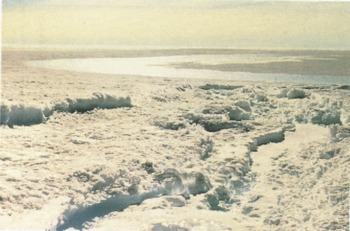
Fig. 2. The dry meltwater-drainage channel surveyed on 13 February 1990. The channel was about 5 m wide and 0.5 m deep, indicating that a significant water discharge must have been drained through this channel. It is unknown whether this flow was produced by “classical” surface melting or by an outburst of meltwater from an upstream frozen lake. The frozen lake and its island of snow located in the middle is seen in the background (from Reference WintherWinther, 1993).
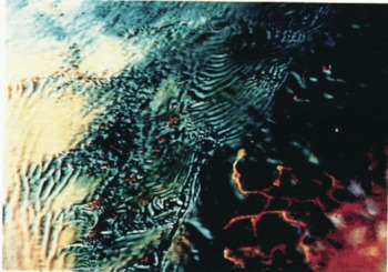
Fig. 3. Colour composite histogram-equalised image of Landsat TM band 5 (red). TM band 4 (green) and TM band 2 (blue) from 12 February 1990. Note the frozen lakes and drainage channels emphasised in the lower right by TM band 5 (red) (from Reference WintherWinther, 1993).
We anticipate that the melt features we have identified in Dronning Maud Land will be quite sensitive to variations in local and regional air temperatures and energy balance. Because of this sensitivity, an understanding and description of the extent and characteristics of these melt features as they change with time can be particularly valuable as climate-change indicators. The programme has thus clearly identified the importance of analyzing how these melting features originate, and of mapping their present areal distribution, determining how sensitive they are to climate change and studying changes in the past and possible changes in the future.
This paper describes our present knowledge of the melting phenomena in Jutulgryta, based on field observations and measurements together with analyses of remotely sensed satellite data. Plans for future work are also presented.
Study Area
The main area of field activity during NARE 1993–94 and the site of an automatic weather station which transfers data via ARGOS is located at 71°24′S, 0°31′E in the Jutulgryta area in Dronning Maud Land. The area lies between the Jutulstraumen ice stream (ν ∼ 700 m year−1) and the slowly moving ice of Hellehallet (ν = 10–100 m year−1) Fig. (1). The ice surface rises from about 100 m.a.s.l. near the grounding line of Jutulstraumen to about 1200 m a.s.l. in the Sverdrupfjella nunatak area to the southeast. Surface undulations in Jutulgryta are about 1–5 km in length and 30–50m in height. During summer, the surface in Jutulgryta consists of patches of snow surrounded by larger areas of blue ice Fig. (4). The snow-covered areas are mainly found in westerly-oriented concave areas. The proportion of snow coverage at Hellehallet increases with altitude up to 500–700 m a.s.l. In this context the lower parts of Hellehallet are considered a part of the Jutulgryta area.
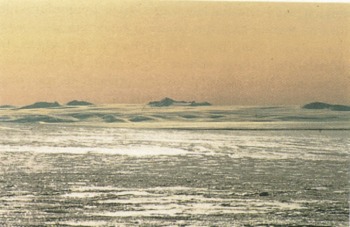
Fig. 4. The Jutulgryta area with its mixed snow and blue-ice fields. The mountains closest to Jutulgryta are located on the other side of the Jutulstraumen ice stream about 80km to the west, and can be seen in the background.
The nearest stations with a climate record are the previous South African bases SANAE I–III which were located 250 km to the west-northwest of Jutulgryta and near the coast. The mean air temperature at SANAE for the period 1957–84 was approximately −17°C (Reference Jones and LimbertJones and Limbert, 1987). Temperatures of 10m boreholes in Jutulstraumen, 200 km southwest of Jutulgryta at 900 m a.s.l. were measured to be about °21°C (personal communication from K.M. Melvold, 1995). The average annual air temperature at Jutulgryta is assumed to be within these limits.
The overall accumulation pattern in Dronning Maud Land shows decreasing accumulation towards the east (Reference LundeLunde, 1961), with increasing distance from the coast (Reference Isaksson and Karlén.Isaksson and Karlèn, 1994). At Norway Station on the Fimbulisen ice shelf, the 1940–59 mean annual accumulation rate was reported to be 50cm w.e. year−1 (Reference LundeLunde, 1961). At 900 m.a.s.l. on the Jutulstraumen ice stream the mean accumulation rate for the last 30 years is calculated as 33 cm w.e. year °1 from one shallow ice core (personal communication from Melvold). In Jutulgryta the accumulation is assumed to be low because of strong easterly katabatic winds (Reference Parish and BromwichParisht and Bromwich, 1987). The mean accumulation in the study area, based on 50 soundings and snow shafts, was 28em w.e. year−1.
Field Observations and Measurements
During NARE 1989–90, observations from helicopter and on the ground confirmed that large-scale melting features are present in this area as first published by Reference Orheim and LucchittaOrheim and Lucchitta (1987, Reference Orheim and Lucchitta1988). A glaciological programme was started on NARE 1993–94 to investigate these melting phenomena more closely.
Surface characteristics and albedo
When the expedition arrived at Jutulgryta on 23 December 1993, the surface was smooth and consisted of dry snow. A few weeks later, surface and sub-surface melting and runoff took place in most of this area. One fundamental reason for this sudden change of surface characteristics was the low winter-snow accumulation in the area. Strong katabatic winds in Jutulgryta keep snow accumulation from below the average in this region. In addition, the Jutulgryta area has a gently north-sloping orientation, making it favourably oriented to incoming solar radiation and thus to ablation.
Snow penitents develop due to the strong incoming solar radiation and favourable local climate. In this area, typical variations in the height of the penitents lie between 10 and 40cm. Their main orientation is east-west, with a pointing angle that corresponds approximately to the elevation of the sun at noon. It is likely that the formation of penitents starts on initial snow ripples (Reference AmstutzAmstutz, 1958) and that most of the penitents in this area can be characterised as micropenitents (Reference LliboutryLliboutry, 1954). The formation of penitents reduces the overall albedo in the area, thus increasing the total absorption of incoming solar radiation on a larger scale, In micro scale (<0.5m), surface reflection will vary substantially when penitents are present. At some point their presence initiates surface melting.
When surface melting first starts, the albedo drops rapidly and the energy available for meltwater production increases correspondingly. At this point several types of surfaces develop, e.g. active (wet) melt pools, inactive or “dead” (dry) melt pools, blue-ice fields, icing from subsurface meltwater that breaks through the frozen top layer and freezes at the cold surface, and a snow/ice mixture where penitents are the dominant feature. Some areas remain snow-covered.. Normally, the melt pools have a diameter of 1–5m. Their life cycle is described in Reference Bøggild, Winther., Sand and HBøggild and others (1995). Albedo values from a transect crossing a melt pool are shown in Figure 5. The surface of a melt pool consists of either open water or a thin ice layer (up to 10cm) or a combination of the two. The usual depth of a melt pool is about 0.5 m. Beneath the melt pool a matrix of loose and corny ice was observed Reference Bøggild, Winther., Sand and HBøggild and others, 1995). After some time, the water level in the melt pools gradually lowers, resulting in a decreasing absorption of solar radiation. As a consequence, the intensity of surface melting decreases, and this leads into an inactive or “dead” stage of the melt pool with respect to surface melting.
In other places the snow cover melts off, exposing a blue-ice surface with low albedo. As described below, subsurface melting and runoff take place in these blue-ice fields. In a lew places sub-surface meltwater is forced towards the surface, where it freezes and causes icing. Melting from areas where penitents are present probably contributes less than the blue-ice fields to the total melt volume. Finally, some areas remain snow-covered. Generally, snow frequently melts and refreezes in these areas, forming a coarse-grained top layer that in a frozen condition typically forms a crust layer 2–5 cm thick.
Surface melting and runoff
A meltwater drainage channel was surveyed onm 13 February 1990 Fig. (2). Similar channels were later detected in a Landsat TM image Fig. (3) recorded on 12 February 1990 (Reference WintherWinther, 1993). The channel observed in Figure 2 was about 5 m wide and 0.5 m deep, indicating that a significant volume of meltwater has been transported through it. Based on the work undertaken prior to NARE 1993–94, it was assumed that surface melting was the only contributor to melting in this area. As described in the next subsection, sub-surface melting probably contributes more to the total melt volume than surface melting does.

Fig. 5. Albedo variations along a 7.1 m long transect that crosses a partly drained melt pool (∆), and at four locations on Lake Jutulsjøen (*). The figure visualises the large span in surface albedo that occurs in this area. Albedo values are integrated numbers obtained from 182 discrete measurements in the wavelength region from 372 to 899 nm. Each measurement represents a bandwidth of approximately 3nm. Measurements were acquired using the portable SE590 spectroradiometer. The field of view of the sensor is 6° and the surface area covered by the sensor represents about 14 cm2 for the measurements presented here (from Reference Bøggild, Winther., Sand and HBøggild and others. 1995).
However, surface melt takes place at all surface types mentioned in the previous subsection. Generally, the meltwater produced during a day (or a few days when night temperatures remain high) freezes during nighttime. This means that melt activity frequently slows down and stops. Observed surface melt and runff during the 1993–94 season was far too limited to explain the large drainage channels seen in this area. However, in December 1991, meltwater flooded large areas in the shear zone between the land ice mass at the Fimbulisen ice shelf close to our study site (personal communication from S. Østcrhus, 1994). This suggests that large year-to-year variations in the intensity of the melt episodes can occur. The possibility that drainage channels are formed from an outburst of their upstream frozen lake should also be considered. At the moment, it is unclear which of the two mechanisms is more important for the formation of meltwater drainage channels.
Sub-surface melting and runoff
Figure 6 shows sub-surface temperature profiles that are about 6°C higher for blue-ice fields (stakes 50 and 53) than for snow (stakes 3, 12 and at the climate station). The temperature profiles seen in Figure 6 are representative for the whole field season (Reference Bøggild, Winther., Sand and HBøggild and others, 1995). Observations from shallow pits confirm that sub-surface melting as well as runoff can occur to depths of about 1 m. The surface remains frozen Fig. (7).

Fig. 6. Measured sub-surface temperature profiles in snowpacks and blue-ice fields in Jutulgryta. The significantly higher ice temperatures (about 6°C) at stakes 50 and 53 refer to registrations in exposed blue ice (from Reference Bøggild, Winther., Sand and HBøggild and others, 1995).

Fig. 7. The photo shows a typical profile in a blue-ice field where sub-surface melting and runoff take place. Note that the surface remains frozen while the runoff layer or aquifer consists of meltwater that drains through a complicated ice matrix. The sub-surface melt layer is normally about 0.5 m deep and was continuously present during 4 weeks of fieldwork in the 1993–94 austral summer season.
The occurrence of a temperature maximum below the surface (the “solid-state-greenhouse effect”) is a result of solar-radiation penetration and absorption inside the ice and the fact that long-wave radiative cooling is restricted to the surface (Reference Brandt and WarrenBrandt and Warren, 1993). The “solid-state-greenhouse effect” has been described theoretically by Reference SchlatterSchlatter (1972) and Reference Brandt and WarrenBrandt and Warren (1993). Brandt and Warren state that the phenomenon is rather questionable within snow but more likely to occur within blue ice, which has a lower extinction coefficient and albedo. Some of the past observations of the “solid-state-greenhouse effect” in snow have been affected by the presence of a dark, absorptive layer such as volcanic ash within the snowpack. No visible contamination could be seen at the surface or in any of the snow/firn pits in Jutulgryta.
Unfortunately, no instruments were brought along to measure runoff volume. However, strong indications that the meltwater produced actually runs off due to gravity force were found by pump tests. Meltwater was pumped out Of auger holes. Flow rates into the auger holes stabilised and remained constant throughout 40min of pumping (Reference Bøggild, Winther., Sand and HBøggild and others, 1995). Thus, it is assumed that sub-surface melting produces a permeable layer that becomes an aquifer for meltwater runoff within the blue-ice fields.
In a few places sub-surface meltwater was directed upwards, resulting in an outflow on the surface. After a while the zero-degree water freezes in contact with the cold surface, producing areas of icing. The size of the icing areas was typically 50–150m2. The physical mechanisms that drive the icing process were not studied.
Frozen lakes
Reference Orheim and LucchittaOrheim and Lucchitta (1987, Reference Orheim and Lucchitta1988) assumed that large “lakes” (1–3 km wide) seen in Landsat TM scenes were open water bodies, possibly covered by a very thin layer of ice. Field observations in February 1990 indicated that the “lakes” were frozen. A visit to such a frozen lake on 13 February 1990 revealed no sign of meltwater at the surface or in the upper part of the frozen lake. The upper 15–20 cm consisted of solid ice which contained some air bubbles and snow crystals. Al that time, it was concluded that the frozen lakes were solid ice bodies that occasionally were fed by meltwater during summer. Further, the hypothesis was that the well-defined drainage meltwater channels that lead into the frozen lakes feed them with meltwater. It was assumed that when meltwater flows out on the frozen lake surface, it spreads out laterally and freezes in contact with the cold ice surface.
However, field measurements from NARE 1993–94 showed that the frozen-lake regime is different and far more complex than first presumed Fig. (1). First, field observations indicate that only a minor part of the meltwater runoff is channelled through the well-defined drainage channels. Most of the meltwater comes from blue-ice fields within the catchment of a frozen lake. This implies that must of the meltwater feeds the frozen lakes through a complicated and dispersed sub-surface runoff system outside the drainage channels. The blue-ice fields that feed the frozen lakes were hardly visible in late December 1993. However, they developed considerably during the next 2–3 weeks. As shown in Figure 5, as soon as blue ice becomes exposed, the albedo drops significantly (Reference Zeng, Cao, X, F, X and WZeng and others, 1984). Consequently, the blue-ice fields act efficiently as solar-radiation traps and can therefore increase relatively quickly in size.
Most of the runoff from the blue-ice fields seems to be sub-surface runoff. On many occasions the blue-ice surface was frozen without any signs of surface melting. Nevertheless, and at the same time, melting and Subsequently meltwater runoff look place in a sub-surface layer within the blue-ice field, as previously explained. A similar phenomenon was reported by Reference EndoEndo (1970) who found under-ice puddles at 10–20cm depth on fast ice (15 m thick) near Syowa Station on the coast of eastern Antarctica. Further, Reference PaigePaige (1968) observed sub surface melt pools on wind-blown blue-ice areas near McMurdo Station, Antarctica. These melt pools were scattered patches of 10–15m in diameter, 7–40cm below the ice surface, and up to 1 m deep. Sub-surface melting can occur because incident solar radiation penetrates to a considerable depth in ice, whereas cooling by the emission of thermal infrared radiation to space occurs at the very top surface of the ice (Reference Brandt and WarrenBrandt and Warren, 1993). Reference Brandt and WarrenBrandt and Warren (1993) concluded that this “solid-state-greenhouse effect” is more favoured in ice than in snow, since ice has lower albedo and a smaller extinction coefficient. The “solid-state-greenhouse effect” was registered in Jutulgryta at NARE 1993–94, and later modelled in Reference Bøggild, Winther., Sand and HBøggild and others (1995). Figure 6 shows a temperature profile that illustrates the presence of the “solid-state-greenhouse effect” in this area.
Eventually, the meltwater meets the bank of a frozen lake. There, as in the blue-ice fields, most of the meltwater flow takes place below the surface. In this case, it means that most of the inflow to lake Jutulsjøen went directly into a sub-surface layer of liquid water 40–83 cm thick. Below this layer, there was solid ice, i.e., most probably the main ice body of the frozen lake. Above this layer, the surface remained frozen with a thickness varying between 10 and 20 cm. The surface was occasionally wetted by meltwater flowing on top of the frozen-lake ice cover. As indicated above, the surface inflow constitutes only a small proportion of the total meltwater inflow to the frozen lake.
This may lead to the conclusion that a “solid-state-greenhouse effect” exists at the frozen lakes as well. A layer of liquid water is present during summer but can hardly remain frozen when temperatures become lower during the austral fall and winter. Thus, there is reason to believe that the frozen lakes consist of solid ice bodies every spring before melting begins.
Satellite Remote-Sensing
Reference Orheim and LucchittaOrheim and Lucchitta (1987) observed lake-like features with albedos close to zero in the six reflective Landsar TM bands in the Jutulgryta area, to our knowledge the first time these frozen lakes have been seen from space. They concluded that the frozen lakes were open water bodies, perhaps covered by a very thin layer of ice. Further, Reference Orheim and LucchittaOrheim and Lucchitta (1987) showed that the lower TM bands were most useful for recognising surface topography, whereas TM bands 5 and 7 were best for distinguishing different types of snow and ice.
Temperature studies using Landsat TM band 6 (Reference Orheim and LucchittaOrheim and Lucchitta, 1988) showed that the frozen lakes were the warmest features in an image which also included nunataks facing the sun. However, the temperatures on the frozen lakes were as low as −8° to −9°C, indicating no presence of water.
During NARE 1989–90, it was observed from both helicopter and ground surveys that these lakes were covered by ice. Later, a Landsat TM scene recorded on 12 February 1990 Fig. (3) simultaneously with field observations was analyzed by Reference WintherWinther (1993). Winther found that a histogram-equalised single TM band 5 image represents a suitable discriminator, leaving frozen lakes and what appeared to be surface meltwater drainage channels as bright areas in the Landsat TM scene. Good contrast between the melting phenomena and the surroundings was obtained, even though the TM band 5 albedo of a frozen lake was calculated to be 0.04, while the nearby snow- and ice-covered areas had a TM band 5 albedo of 0.03 Fig. (3). In spite of the small absolute difference in albedo, the large relative albedo difference favoured the use of histogram-equalising and made it possible to emphasise these features.
Sensitivity of Temperatures in Blue-Ice Fields
In the mixed snow-and-ice zone in Jutulgryta, the downslope flow of ice can cause snow-covered ice to become exposed at some stage, resulting in the rise of sub-surface temperatures, as shown in Figure 6. The following analysis will focus on the modelling of ice temperatures when a sudden exposure of blue ice appears on previously snow-covered surfaces.
To simulate the evolution of ice temperatures, the model of Reference Bøggild, Winther., Sand and HBøggild and others (1995) has been used. The original model has been modified by coarsening the grid resolution when simulating temperature developments over several years. At 15 m depth, ice temperatures have been kept constant as initial conditions in the model. The temperature profile from stake 3 in Figure 6 has been used as initial conditions, however, with the same thermal and optical properties as for blue ice. As forcing and upper-boundary conditions in the model, monthly mean values for air temperatures and global radiation from the German Georg von Neumayer (GvN) station have been used. Annual mean temperature measurements for 10 years from GvN differ only by 0.3°C from the deepest (8.5 m) firn temperature recorded in Jutulgryta in January 1994. With the GvN research station located about 250 km west of Jutulgryla but at approximately the same elevation and latitude, the annual cycles of air temperatures in Jutulgryta can be assumed to be similar to those at GvN.
The simulations in Figure 8 show that several years of exposed blue ice are needed to produce the rise of temperatures from the “cold” snow-covered profile to the “warm” ice temperatures of exposed blue ice seen in Figure 6. The trend is clear, but interpretation cannot be carried further due to the lack of observations during winter. In order for temperatures to have risen by 6°C Fig. (6), it is possible that sub-surface melting in blue-ice fields in Jutulgryta has occurred for many years. Initiation and termination temperatures at mid-austral winter (1 July, Fig. 8) further show that the effect of ice-warming during the sub-surface melt season remains during the winter and is still detectable the following year. This results in a cumulative warming of the ice and a parallel rise in ice temperatures Fig. (8). It is also clear from Figure 8 that the temperature increase from year to year decreases with time, i.e. the blue-ice-field temperature profile will eventually approach an equilibrium after more than 8 years.
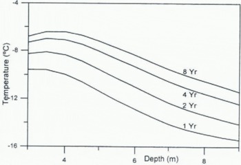
Fig. 8. Model simulations of temperatures in a blue-ice field when the radiative “protecting” snow cover is removed. The simulations indicate that a sudden exposure of blue ice will increase ice temperatures by several degrees Celsius. Combined with the measured temperature differences between snow and blue ice seen in Figure 6. this implies that these blue-ice fields have been exposed for many years.
The effect of the reported ozone hole over Antarctica on sub-surface melting is questionable. It is likely that increased penetration of ultraviolet (UV) radiation through the atmosphere will further enhance radiation absorption in blue ice since the ice is most transparent to solar-radiation penetration in the short-wave range and becomes increasingly opaque with longer wavelengths (Grenfell and Maykut, 1977). One can speculate that an increased UV radiation may trigger further development of areas where sub-surface melting and runoff take place. On the other hand, this will be restricted to areas where favourable conditions for increased exposure of blue ice exist, such as areas of low snow accumulation.
Further Work
Future work falls into three main categories. The first consists of field measurements and data analyses of local and regional hydrologic characteristics by (1) collecting and analyzing ground-truth data, e.g. GPS for positioning of melt features, snow/ice characteristics, slope and aspect together with surface reflectance and temperature for satellite-image interpretation; (2) studying the hydrologic regime in the Jutulgryta area, e.g. melting, drainage, runoff, frozen lakes and vertical temperature profiles; (3) performing and analyzing radio-echo soundings of melt features to obtain their three-dimensional characteristics; and (4) Carrying out and analyzing shallow ice cores to obtain snow-accumulation data.
The second category comprises field measurements and data analyses of local and regional surface energy balance and meteorological characteristics. These will be performed by (1) studying melt processes, in particular sub-surface melting: (2) collecting and analyzing year-round meteorological data; (3) measuring visible and infrared surface reflectance for energy-balance calculations, including spectral reflectance; and (4) analyzing spectral UV data for estimating the impact that changes in the ozone layer may have on surface energy exchange and the development of melt features.
The third category consists of the development of a methodology to study past and potential future changes in the melt-related features in the Jutulgryta area and the use of the methodology for other coastal regions of Antarctica. This work will be carried out by (1) analyzing optical and radar-satellite remote-sensing data combined with ground-truth data to analyze characteristics and areal distribution of the melt features in Jutulgryta, and (2) developing algorithms that can be used for other coastal Antarctic melt regions.
Conclusions
Large-scale melting phenomena such as meltwater drainage channels and meltwater accumulation basins or frozen lakes are present on the land ice mass in Jutulgryta. Dronning Maud Land. The largest frozen lakes are 2–3 km wide, while some of the surface drainage channels stretch more than 5 km. Snowmelting at such a rate that meltwater flows in the drainage channels surveyed is probably infrequent. However, this occurs occasionally during periods of favourable meteorological conditions and probably when an outburst of meltwater from an upstream frozen lake occurs. The surface melt features are detectable by satellite remote-sensing techniques. They can be thrown into relief by applying processing techniques such as principal component analysis, band ratioing, and histogram-equalising. In particular, Landsat TM band 5 seems to be a good discriminator.
The presence of sub-surface melting and runoff was found throughout the 1993–94 field season (4 weeks). Subsurface melting is a result of solar-radiation penetration and absorption inside the ice, and long-wave radiative cooling of the surface, i.e. the “solid-state-greenhouse effect”. The phenomenon develops in blue-ice fields where there is a very low winter snow accumulation. There are no signs of an internal absorbing layer such as volcanic ash in Jutulgryta. Since the surface remains frozen in the areas where sub-surface melting takes place, the phenomenon is invisible to the human eye. Thus, this kind of melting can take place over larger areas and in other regions than studied in this particular programme. Radar satellite sensors will be used to further investigate and map the areal distribution of areas of sub-surface melting.
The conditions necessary for melting to take place in Jutulgryta are probably marginal. A slight increase in air temperature can result in more “classical” surface melting, whereas a cooling may disable sub-surface melting. Surface melting in this area is limited and insignificant for the mass-balance budget. However, we anticipate that the sub-surface melt-related features we have identified in Dronning Maud Land are quite sensitive to variations in local and regional air temperature and energy balance. Because of this sensitivity, an understanding and description of the extent and characteristics of these melt features as they change with time can be particularly valuable as climate-change indicators. An analysis of the origin of these melt features, mapping of their present areal distribution, determination of their sensitivity to climate change, and a study of past and possible future changes are all vitally important research areas identified by this programme.
Acknowledgements
The authors would like to thank the Svensk Polarfors-kningssekretariatet for the excellently organised expedition under the Nordic Antarctic Research Programme 1993–94 (NARP 93–94). All the participants on NARP 93–91 are also acknowledged, together with the Norsk Polarinstitutt which was responsible for organising the participation of the Norwegian research groups. This project was funded by the Research Council of Norway, the Danish Natural Science Research Council and by NorFa. This is publication No. 143 of the Norwegian Antarctic Research Fxpeditions (1993–94).


