


1. Introduction
Considerable effort is being made to develop and improve statistical models that increase cross-validation accuracy in genome-wide association studies or genome-assisted prediction of phenotypes. Bayesian methods, which use shrinkage to estimate regressions of phenotypes on single nucleotide polymorphism (SNP) genotypes, have gained attention for this purpose. However, some of the Bayesian specifications proposed have statistical drawbacks, such as strong assumptions on the prior distribution of marker variance, or difficulties in capturing complex SNP signals (Gianola et al., Reference Gianola, de los Campos, Campos, Manfredi and Fernando2009). Besides, these methods may lose accuracy when markers are sparse, e.g. with low-density genotyping or when pre-selection of SNPs is practiced (Solberg et al., Reference Solberg, Sonesson, Woolliams and Meuwissen2008; Weigel et al., Reference Weigel, de los Campos, González-Recio, Naya, Wu, Long, Rosa and Gianola2009). This may be important when predicting genomic breeding values in populations in which large-scale genotyping is available (e.g. cattle and poultry), or for tagging SNPs in diagnosis of genetic diseases (Lowe et al., Reference Lowe, Cooper, Chapman, Barratt, Twells, Green, Savage, Guja, Ionescu-Tîrgovişte, Tuomilehto-Wolf, Tuomilehto, Todd and Clayton2004). Non-parametric (NP) methods seem to be less influenced by marker density (Gianola et al., Reference Gianola, Fernando and Stella2006; Gonzalez-Recio et al., Reference Gonzalez-Recio, Gianola, Long, Weigel, Rosa and Avendaño2008, Reference Gonzalez-Recio, Gianola, Rosa, Weigel and Kranis2009). However, this class of methods has not yet gained as much attention as Bayesian linear regression methods, probably because their interpretation is less straightforward and, depending on the implementation, may be computationally more complex.
The use of methods that involve some sort of variable selection is pertinent in problems with a large number of predictor variables, such as genomic selection. Machine-learning algorithms have been introduced in a genomic selection context (Long et al., Reference Long, Gianola, Rosa, Weigel and Avendaño2007), and these may be useful for increasing the accuracy of predictions using pre-selected SNPs in prediction models (Szymczak et al., Reference Szymczak, Biernacka, Cordell, González-Recio, König, Zhang and Sun2009). Boosting is a procedure that has not yet been studied in a genomic selection context. It is a machine-learning ensemble method, which means that several models are somehow combined to improve the predictive ability. The manner in which models are combined, labels the ensemble method (e.g. model averaging, bagging or boosting). The original AdaBoost algorithm (Freund & Schapire, Reference Freund, Schapire and Saitta1996) and modifications thereof have attracted much attention in several fields of science, due to their good empirical performance. These algorithms have been shown to be powerful in classification problems (Opitz & Maclin, Reference Opitz and Maclin1999). One of the most interesting modifications is the L 2-Boosting algorithm for regression in high-dimensional problems, which also has advantages when a non-null covariance structure between explanatory covariates exists, e.g. SNPs in high linkage disequilibrium. This version of boosting considers an L 2 loss function in a recursive fashion, and its statistical properties and performance have been described by several authors (e.g. Bühlmann, Reference Bühlmann2006; Lutz et al., Reference Lutz, Kalisch and Bühlmann2008).
The objectives of this study were: (1) to apply L 2-Boosting with two different weak learners in two different genome-assisted genetic evaluation scenarios and (2) to compare L 2-Boosting with BayesA and BL [Bayesian LASSO (least absolute shrinkage and selection operator] models, which are methods commonly used to compute genome-assisted evaluations. This provides a strong test of the hypothesis of whether or not L 2-Boosting with weak learners can attain the predictive ability of complex Bayesian hierarchical models.
2. Material and methods
(i) Data
Two data sets from different species (dairy cattle and broilers) were analysed. These data sets are briefly described next.
(a) Dairy cattle
High-density SNP genotypes of 4702 Holstein sires, which were derived from the Illumina® BovineSNP50 BeadChip, and their respective progeny test predicted transmitting abilities (PTAs) for the length of productive life (PL), were obtained from the Bovine Functional Genomics Laboratory and Animal Improvement Programs Laboratory, respectively, at the USDA-ARS Beltsville Agricultural Research Center (Beltsville, MD). The aforementioned PTAs were computed using a genetic evaluation model that assumes the existence of an infinite number of loci, each with an infinitesimally small additive effect. Genotypes at each SNP locus were coded arbitrarily as 0 (homozygous for allele B), 1 (heterozygous), 2 (homozygous for allele b) or 5 (missing). The 38 416 SNPs used in the study of VanRaden et al. (Reference VanRaden, Van Tassell, Wiggans, Sonstegard, Schnabel, Taylor and Schenkel2009) were edited further. Monomorphic SNPs, SNPs with minor allele frequency (MAF) <0·05, and SNPs with >10% missing genotypes were excluded from the analyses. Information from flanking markers was used to impute the most probable genotypes for other loci with missing genotypes, based on the conditional probability of observing a particular configuration at a locus in question given genotypes at both neighbouring markers. This led to a total of 32 611 SNPs for the analyses described herein. The data were split such that a training data set contained ancestors and contemporary individuals, and a testing set represented the progeny of these individuals whose phenotypes (PTAs) were regarded as yet to be observed. The training set included PL PTAs (standardized to attain a distribution with a null mean and variance equal to 1) from the 2003 routine genetic evaluation of 3304 sires born before 1998. The testing set included the standardized PL PTAs from the 2008 routine genetic evaluation of 1398 sires born after 1998. Further details on this data set are in Weigel et al. (Reference Weigel, de los Campos, González-Recio, Naya, Wu, Long, Rosa and Gianola2009).
(b) Broilers
The data consisted of average food conversion rate (FCR) records of the progeny of 394 sires from a commercial broiler line in the breeding program of Aviagen Ltd (Newbridge, Scotland, UK). Prior to the analyses, the individual bird FCR records were adjusted for environmental and mate of sire effects. Genotypes consisted of 4505 SNPs distributed along the genome. All SNPs with monomorphic genotypes or with MAF <5% were excluded. After editing, genotypes consisted of 3481 SNPs. The data set was also split into training and testing sets. Sires included in the testing set were required to have more than 20 progeny with FCR records to ensure a reliable mean phenotype, and they were required to have sires in the training set. Sixty-one sires (15·5% of the total) were included in the testing set, whereas the remaining 333 sires were in the training set. Predictions were calculated from the training set, and the accuracy of predicting the mean progeny phenotype was assessed using sons in the testing set. More details on this data set can be found in Gonzalez-Recio et al. (Reference Gonzalez-Recio, Gianola, Rosa, Weigel and Kranis2009).
In the two data sets, the same families could be represented in both training and testing sets, so the procedures utilize both linkage disequilibrium and linkage information. Clustering different families within either training or testing sets is difficult when using livestock data, because families and generations usually overlap. From a genomic selection point of view, the approach utilized herein is realistic, because the typical objective is to determine which sires are to be chosen from the current population for use as parents of the next generation.
(ii) L2-Boosting for high-density genotypes
This learning technique is based on the AdaBoost algorithm described by Freund & Schapire (Reference Freund, Schapire and Saitta1996), and it combines several weak learners to form a ‘committee’ with potentially greater predictive ability than that of any of the individual learners. A weak learner is defined as a predictive method with a slightly better performance than random guessing. Although boosting was originally designed for classification problems, it was extended to regression by Friedman (Reference Friedman2001). Bühlmann & Yu (Reference Bühlmann and Yu2003) proposed a version of boosting with the L 2 loss function for regression and classification, which is called L 2-Boosting. The L 2 loss function measures the degree of wrongness of the predictions using a quadratic term with the form L 2 loss=f(y−ŷ)=(y−ŷ)2. The authors also showed that L 2-Boosting may be used for regression in high-dimensional problems by doing some type of covariate selection through a small-step gradient descent. The L 2-Boosting algorithm for regression problems involving s genomic markers (with s being very large and possibly s>>n, where n is the training sample size) is described next.
Consider the model
where y is an n×1 vector of records; xp is a vector of genotype codes of n individuals for the SNP locus p; g(xp) is an unknown function to be learned and interpretable as E(y|xp) and e is a vector of residuals assumed to be identically and independently distributed, and also independent of xp. Different learners may be used to learn about g(xp). Here, two different learners (linear and non-linear) were employed. The linear learner was ordinary least squares (OLS; OLS-BOOST) regression, and the non-linear learner was NP (NP-BOOST) regression. A priori, NP would be expected to capture both additive and non-additive signals. Once the learners have been set, the boosting algorithm works as follows:
Step 1 (Initialization): Given the data (y, x), apply the weak learner procedure to each SNP one at a time, yielding the function estimate f o(⋅)=ĝ(xp), where ĝ(xp) is estimated from the original data set, with ![]() . Set m=1. Let the prediction of phenotypes be
. Set m=1. Let the prediction of phenotypes be ![]() .
.
Step 2. Compute residuals as ![]() , and fit the weak learner for each SNP p(p∊1, …, s) to current residuals, where v is a shrinkage parameter describing the step size when updating the residuals. Without loss of generality, v can be assumed as constant and small (0<v<1), but it may be optimized to balance the predictive ability and computation time. Select SNP p, where
, and fit the weak learner for each SNP p(p∊1, …, s) to current residuals, where v is a shrinkage parameter describing the step size when updating the residuals. Without loss of generality, v can be assumed as constant and small (0<v<1), but it may be optimized to balance the predictive ability and computation time. Select SNP p, where ![]() and set f m(⋅)=ĝ(xp). Here, v equal to 0·1 and 0·01 was used for OLS-BOOST and NP-BOOST, respectively.
and set f m(⋅)=ĝ(xp). Here, v equal to 0·1 and 0·01 was used for OLS-BOOST and NP-BOOST, respectively.
Step 3. Update predictions as ŷmi=ŷ m−1i+fm(ri, x i,p), (i∊{1, …, n}), where fm(r i, x i,p) is the estimate for individual i obtained by regressing the current residual (ri) at iteration m on its genotype for SNP p (x i,p).
Step 4. Increase the iteration index m by 1, and repeat steps 2–4 until a convergence criterion is reached.
As stated, the two weak learners used were OLS-BOOST and NP-BOOST. The NP learner is less commonly known and a description is given in Appendix A. Boosting yields an additive model whose terms are fitted in a stepwise fashion. Note that the function g(xp) does not assume linearity when using NP- BOOST.
Boosting algorithms for regression have been interpreted as functional gradient descent techniques (Bühlmann, Reference Bühlmann2006), and L 2-Boosting may be viewed as a sequence of Hilbert spaces in what is known as a ‘weak greedy algorithm’. Boosting is one of the most successful and practical methods in the machine-learning field. It has great flexibility and can capture complexity introduced by covariates, such as SNPs. Although it was first thought as a black box, its statistical properties have been described by some authors (Bühlmann, Reference Bühlmann2006; Cornillon et al., Reference Cornillon, Hengartner and Matzner-Lober2008).
(iii) Convergence criterion
This can be viewed as a model selection problem, and stopping rules based on criteria such as the Bayesian Information Criterion (BIC), Akaike Information Criterion (AIC), a corrected version of AIC (AICc), or generalized cross validation (GCV) can be used. Other criteria have been proposed, but there is some consensus on the benefits of GCV (Bühlmann, Reference Bühlmann2006; Cornillon et al., Reference Cornillon, Hengartner and Matzner-Lober2008; Lutz et al., Reference Lutz, Kalisch and Bühlmann2008). In this study, a 10-fold cross validation was utilized to tune the optimal number of iterations, as follows. Ten per cent of the observations, which were randomly sampled from the training set, were kept as the tuning set. Steps 1, 2 and 3 of the boosting algorithm were performed on the training set, without including observations of the tuning set. The convergence criterion (Step 4) was determined as follows. Mean-squared error (MSE) was computed in the tuning set at each iteration as
where t is the number of individuals in the tuning set, yj is the observed response of individual j in the tuning set and ŷ j is its predicted response calculated at each iteration after selecting the SNPs that minimized MSE in the training set. The optimal number of iterations was that which minimized MSE in the tuning set, after running a large enough number of iterations. Note that the training set was used to make the inferences, and the tuning set to determine the iteration at which the algorithm would be stopped.
Predictions in the testing set were computed at the optimal iteration. Since a 10-fold GCV was used, 10 independent tuning sets were created in 10 different analyses, and predictions in the testing set were averaged across runs. Note that this GCV scheme creates independence between the testing and tuning sets. The maximum number of boosting iterations was set to 5000. An illustration of the algorithm framework is given in Fig. 1.
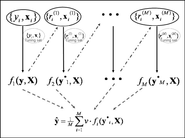
Fig. 1. Schematic diagram of the boosting framework. Each weak learner fm(y, X) is trained on a weighted form of the training set (![]() ), which are the residuals from the previous weak learner (
), which are the residuals from the previous weak learner (![]() ). The weak learner is tested on a tuning set at each iteration. Once all weak learners have been trained, those from iteration 1 to that minimizing MSE in the tuning set are combined to provide final estimates ŷ (
). The weak learner is tested on a tuning set at each iteration. Once all weak learners have been trained, those from iteration 1 to that minimizing MSE in the tuning set are combined to provide final estimates ŷ (![]() ). Adapted from Bishop (Reference Bishop2006).
). Adapted from Bishop (Reference Bishop2006).
These two boosting algorithms were compared with BayesA and BL, two methods that have received attention in genomic selection (Meuwissen et al., Reference Meuwissen, Hayes and Goddard2001; de los Campos et al., Reference de los Campos, Naya, Gianola, Crossa, Legarra, Manfredi, Weigel and Cotes2009; Weigel et al., Reference Weigel, de los Campos, González-Recio, Naya, Wu, Long, Rosa and Gianola2009). Details on BayesA and BL are given in Appendices B and C, respectively. For these methods, a tuning set is not necessary and the whole training set was used for inferences.
There is some similarity between L 2-Boosting and LASSO. However, these methods differ as shown by Bühlmann (Reference Bühlmann2006), and a different variance-bias trade-off is achieved by each approach. They also differ in the maximum number of predictor variables allowed in the model. The maximum number of covariates selected by the original LASSO, as proposed by Tibshirani (Reference Tibshirani1996), is min(n, s+1) including an intercept, where s is the number of covariates. In the Bayesian counterpart of LASSO (Park & Casella, Reference Park and Casella2008), all estimates of regressions on markers are shrunk towards zero (but never set to exactly zero) using a conditional Laplace prior assigned to regression coefficients. In this case, the maximum number of influential covariates is s, and an ad-hoc threshold must be used to set the number of desired covariates, if so desired. On the other hand, the number of covariates selected in L 2-Boosting depends on the number of iterations until the chosen convergence criterion is reached, and a particular covariate could be selected several times or might not be selected at all.
(iv) Validation criteria
Correlations between true and predicted phenotypes and MSE for each method were calculated. Larger correlations and smaller MSE values indicate better performance of the model. Bias was calculated as ![]() , where s is the number of individuals in the testing set. A priori, a method with smaller bias is preferable unless its variance is too large.
, where s is the number of individuals in the testing set. A priori, a method with smaller bias is preferable unless its variance is too large.
Realized observations in the testing set (ytest) were regressed on their predictions (ŷtest) as
where a is the intercept, b is a regression coefficient and ε is a residual. An unbiased method is expected to have a=0 and b=1. Values of the slope that are above or below one would indicate under-prediction or over-prediction, respectively.
3. Results and discussion
The estimated shrinkage parameter λ of BL was 205·9 for the dairy cattle data set and 69·5 for the broiler data set, with posterior standard deviations equal to 2·4 and 2·2, respectively. These estimates suggest greater shrinkage in the dairy data, which was expected due to the larger number of markers in this data set. The average time per iteration (calculated in the same workstation) in the dairy cattle data set was 12·4 s for BayesA, 12·1 s for BL, 3·4 s for OLS-BOOST and 4·1 h for NP-BOOST; whereas 0·04 s were needed for BayesA, BL and OLS-BOOST and 16·66 s for NP-BOOST in the broiler data set. Note also that the number of iterations needed was lower for the boosting algorithms. OLS-BOOST required less computer time than the other methods, which may be an advantage when using large data sets with several thousands or millions of markers. The NP-BOOST algorithm seemed to be too time-consuming in large data sets. Nonetheless, the time per iteration is dependent on hardware and software used.
Figures 2 and 3 show the MSE obtained for each fold of GCV in the tuning set at each iteration of OLS-BOOST and NP-BOOST in the cattle and poultry data sets, respectively. These plots allow the visual inspection of convergence of the boosting algorithm. With a smaller step size (υ), the algorithm converged more slowly. OLS-BOOST (MSE=0·96) had better performance than NP-BOOST (MSE=1·23) in the dairy cattle tuning set. It must be pointed out though that NP-BOOST was not optimized in this data set, because the computation time per iteration was prohibitive. Because of slow convergence, the step size υ=0·01 in NP-BOOST was increased to υ=1, resulting in under-performance of this weak learner. It is essential to monitor the tuning set, because L 2-Boosting often yields the fully saturated model, which fits the training data perfectly, and the bias and prediction variance explode as iteration proceeds (Bühlmann & Yu, Reference Bühlmann and Yu2003). Initial iterations of the algorithm are expected to have a large bias and a low prediction variance. As the model becomes more complex, with a larger number of SNPs having a non-zero effect, the algorithm uses the training set more effectively and is able to adapt to more complicated underlying genetic systems. This may lead to lower bias but higher variance, which suggests over-fitting in the training set. Hence, the algorithm must be stopped at an iteration that provides intermediate complexity for the prediction of future records.
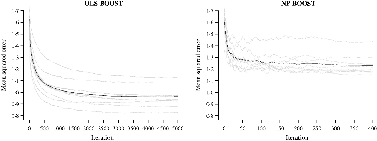
Fig. 2. MSE at each iteration for OLS-BOOST and NP-BOOST in the dairy cattle tuning set in each of the 10 folds (grey line) and the averaged MSE across folds (black solid line).
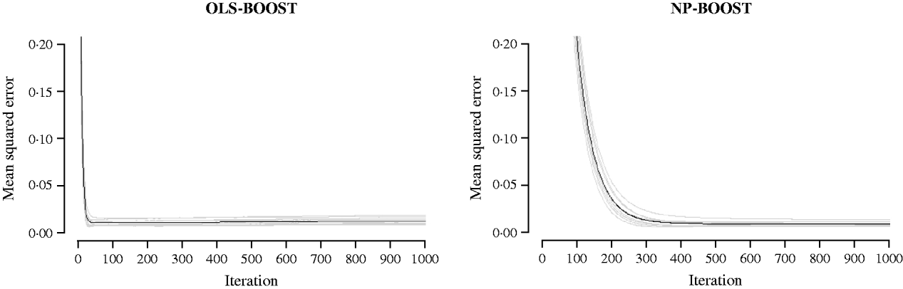
Fig. 3. MSE at each iteration for OLS-BOOST and NP-BOOST in the broiler tuning set in each of the 10 folds (grey line) and the averaged MSE across folds (black solid line). For convenience, only the first 1000 iterations are shown.
Pearson correlations of predictions obtained with each method in the testing sets are shown in Table 1. Pearson correlations between predicted and observed phenotypes were similar for all methods in the dairy cattle data set, ranging between 0·63 and 0·66, except for NP-BOOST, which yielded a Pearson correlation of 0·53 without optimizing the algorithm, due to the computation time, as stated above. These correlations were similar to those obtained by VanRaden et al. (Reference VanRaden, Van Tassell, Wiggans, Sonstegard, Schnabel, Taylor and Schenkel2009), who regressed daughter yield deviations for PL on 40 426 SNPs in a sample from the same Holstein population using a linear Bayesian regression model with an adjustment for the reliability of parent average. In the broiler data, L 2-Boosting produced larger Pearson correlations (OLS-BOOST=0·33 and NP-BOOST=0·37) than those obtained with Bayesian regressions (0·26–0·27). The L 2-Boosting algorithm with NP as a weak learner had up to 42% greater accuracy than the linear Bayesian regression models using progeny means as response variables in the broiler data set. In this data set, the NP weak learner outperformed OLS in prediction accuracy, suggesting that it may capture more genetic (additive and non-additive) variance from the data.
Table 1. Pearson correlation between yet to be observed records and their predictions in each testing set for L2-Boosting with OLS regression or NP regression as weak learners, BayesA and BL
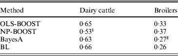
1 Results not optimized due to large computation time per iteration.
2 Results from Gonzalez-Recio et al. (Reference Gonzalez-Recio, Gianola, Rosa, Weigel and Kranis2009).
The Pearson correlation obtained with L 2-Boosting was larger than those obtained by Gonzalez-Recio et al. (Reference Gonzalez-Recio, Gianola, Rosa, Weigel and Kranis2009) and Long et al. (Reference Long, Gianola, Rosa, Weigel, Kranis and González-Recio2010) using different models on the same data set. However, confidence intervals presented by Gonzalez-Recio et al. (Reference Gonzalez-Recio, Gianola, Rosa, Weigel and Kranis2009) overlapped with those obtained in this study, and Long et al. (Reference Long, Gianola, Rosa, Weigel, Kranis and González-Recio2010) found a slightly smaller MSE using radial basis functions.
Bias and MSE of predictions from each method are shown in Table 2. The OLS-BOOST algorithm had the smallest MSE (1·08) in the dairy cattle testing set followed by BL (1·10), and in the broiler data set (0·006) followed by NP-BOOST (also 0·006). BayesA had the poorest MSE (2·81) in the dairy cattle data set, and this was almost 2·6 times greater than the MSE obtained with OLS-BOOST. However, in the broiler data set, MSE was similar for all four methods, with a slight advantage for boosting. OLS-BOOST and BL produced the smallest bias in both dairy cattle (0·08 and 0·10, respectively) and broiler (−0·011 and −0·010, respectively) data. BayesA and NP-BOOST had the largest bias in the dairy cattle (1·26, 0·57) and broiler (−0·016, −0·018) data sets. Differences in bias between OLS-BOOST and BL in the dairy cattle data set have to be taken cautiously, as phenotype distributions in the training and testing data sets were normalized and centred, ignoring the genetic trend that, although small, may exist.
Table 2. Bias and MSE of predicted responses in each testing set for L2-Boosting with OLS regression or NP regression as weak learners, BayesA and BL
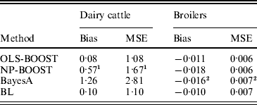
1 Results not optimized due to large computing time per iteration.
2 Results from Gonzalez-Recio et al. (Reference Gonzalez-Recio, Gianola, Rosa, Weigel and Kranis2009).
The Bayesian regression methods estimated the slope of the regression of observed on predicted values at 0·71 and 1·34 in the dairy cattle data set (Fig. 4). Bayesian regression methods produced smaller slopes (0·36) in the broiler data set (Fig. 5). These results suggest better agreement between observed responses and their predictions obtained with L 2-Boosting. The BL and BayesA tended to underestimate the true progeny means in the broiler data, whereas OLS-BOOST overestimated them.
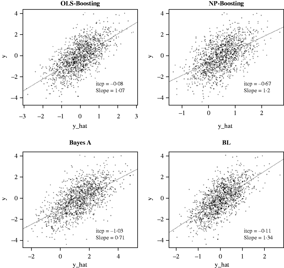
Fig. 4. Relationship between 2008 progeny test PTA for productive lifetime (y) and 2003 genomic PTA (y_hat) in a testing set comprised 1398 Holstein bulls born from 1999 to 2002 using L 2-Boosting with OLS regression or NP regression as weak learners, and with BayesA and BL. Intercept and slope estimates from the linear regressions are given.
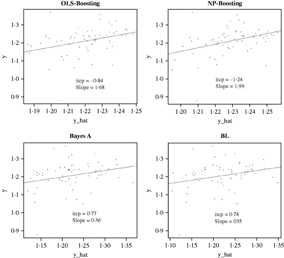
Fig. 5. Relationship between observed average FCR, adjusted by environmental and mate effects, (y) and the genomic predicted FCR (y_hat) in a testing set comprised 61 broilers, which were progeny of 394 broilers in the training set using L 2-Boosting with OLS regression or NP regression as weak learners, and BayesA and BL. Intercept and slope estimates from the linear regressions are given.
Similar regression coefficients ranging between 0·71 and 0·86 have been found by other authors (VanRaden et al., Reference VanRaden, Van Tassell, Wiggans, Sonstegard, Schnabel, Taylor and Schenkel2009; Aguilar et al., Reference Aguilar, Misztal, Johnson, Legarra, Tsuruta and Lawlor2010) for overall conformation, working with a similar population but using different versions of the so-called ‘genomic BLUP’ (VanRaden, Reference VanRaden2008). Aguilar et al. (Reference Aguilar, Misztal, Johnson, Legarra, Tsuruta and Lawlor2010) obtained a regression of observed on predicted response of 0·86 using a single-step approach with phenotypes from several million animals. Results obtained with OLS-BOOST in this study were similar to those recently reported by the USDA for the same trait (the squared correlation was 0·31 and the slope of the regression was estimated at 1·08), but that study used a larger number of records and used daughter yield deviation as response variable, instead of the PTA values used here.
In summary, BL and OLS-BOOST had better predictive ability in the dairy cattle data set than BayesA and NP-BOOST. The two former methods provided greater accuracy (larger Pearson correlation and smaller MSE), with some advantages for OLS-BOOST in terms of bias. In the broiler data set, L 2-Boosting provided the highest correlations and smallest MSE of prediction of yet-to-be observed phenotypes although NP-BOOST showed some bias. It must be pointed out that the need for a tuning set in the L 2-Boosting algorithm may be a disadvantage relative to BL and BayesA, which use the whole training set for making inferences. The main difference between L 2-Boosting and other methods commonly used, such as partial least squares, Bayesian regressions or reproducing kernel Hilbert spaces is that L 2-Boosting is trained using a sequence of residuals from previous iterations in a weighted fashion. Only the covariate (SNP) that minimizes the loss function is used at each iteration, and a small step is taken towards modelling the real observations.
Differences between these data sets must be emphasized. The dairy cattle data set had a larger number of data points and SNPs, and its response variable was PTAs predicted from a model that assumed additivity and normality, which is expected to reflect additive genetic effects only, instead of the average progeny performance,. Also, as stated earlier, a PTA is a smoothed product from a predictive model which may hide signals that are actually present in the data, although it is expected to account for some part of epistatic variance acting in an additive manner (Hill et al., Reference Hill, Goddard and Visscher2008). It must be pointed out that PTA may also include a contribution from parents’ information.
Several authors have shown that boosting may increase accuracy in regression analysis. For example, Friedman (Reference Friedman2001) and Opitz & Maclin (Reference Opitz and Maclin1999) reported benefits of boosting using 23 different data sets, indicating that it can create ensembles that are often more accurate than those from other ensemble methods, such as bagging (Breiman, Reference Breiman1996). However, Opitz & Maclin (Reference Opitz and Maclin1999) also showed that the Ada-Boosting algorithm may be sensitive to noisy data and may be prone to over-fitting, although this was later questioned by Bühlmann & Yu (Reference Bühlmann and Yu2006).
Results from our study suggest that performance of L 2-Boosting may depend on the weak learner chosen and the step size used. We used two arbitrarily chosen weak learners from a large variety of candidates, and the performance of each may depend on the underlying problem (state of nature). Further, a small value of the step-size parameter (υ) should be used for convenience, but it can be optimized, if possible, when computing time is a limiting factor. Smaller values of υ increase the degree of weakness of a learner. Smaller values of υ were tested for both learners (results not shown), without improving accuracy, but with a corresponding increase in the computing time (except for NP-BOOST in the dairy cattle data set, as noted above).
The results obtained in this study should hold provided there is genetic or molecular similarity, whereas the absence thereof may yield different performance, but this must be evaluated on a case-by-case basis.
4. Conclusions
Our results highlight the potential ability of L 2-Boosting of attaining high accuracy and small bias in high-dimensional problems, such as genomic selection, when a suitable weak learner is used. This makes such algorithms appealing for selecting signal covariates in whole-genome studies. L 2-Boosting seemed to be appealing for scenarios in which more noise exists. BL may yield similar accuracy as L 2-Boosting under linear and additive scenarios. In a genomic selection context, a higher correlation between predicted and observed responses is desirable, and the boosting algorithm seemed competitive in this regard. Other methods commonly used in genomic-assisted evaluation yielded similar accuracy, as shown here and in recent scientific literature. However, unbiased and reliable predictions are necessary to compare animals or plants in commercial breeding programmes. Differences in MSE and bias may assist in determining which method is preferred for the prediction of individual total genomic merit of the traits of interest in a given species.
Overall, L 2-Boosting seems to be a viable alternative to more widely used methods of the prediction of the total genomic merit of animals and plants that are candidates as parents of future generations. However, its promising behaviour must be studied further in a whole genomic evaluation context. Among other issues, the choice of weak learner, stopping criterion, step-size parameter and programming strategy (such as parallelization) may be considered in future studies to improve the performance of the algorithm.
AVIAGEN Ltd, Newbridge, Scotland, is thanked for providing the broiler data. The authors gratefully acknowledge scientists at the USDA-ARS Beltsville Agricultural Research Center for proving genotypic and phenotypic data. The expertise of C. P. Van Tassell, P. M. VanRaden and J. R. O'Connell was greatly appreciated. K.W. acknowledges financial support from the National Association of Animal Breeders (Columbia, MO), and O.G.-R. acknowledges financial support from the UW-Madison Babcock Institute for International Dairy Research and Development. This project was partially funded by National Research Initiative Grant No. 2009-35205-05099 from the USDA Cooperative State Research, Education and Extension Service.
Appendix A
A NP regression on genomic markers for animal breeding was proposed first by Gianola et al. (Reference Gianola, Fernando and Stella2006) and applied to chicken mortality by Gonzalez-Recio et al. (Reference Gonzalez-Recio, Gianola, Long, Weigel, Rosa and Avendaño2008). Consider the model
where y=yi is the (n×1) vector of responses and xi is a (n×1) vector representing the genotype of individual i (i∊{1, …, n}) for p SNP loci. Here, g(xi) is some unknown function representing the expected response value of individuals with SNP genotype xi, i.e. the conditional expectation function E(y|xi). The random vector of residuals, e=ei, is assumed identically and independently distributed. Here, the conditional expectation function given a vector of codes for the SNP locus p
was inferred using the Nadaraya–Watson estimator (Nadaraya, Reference Nadaraya1964; Watson, Reference Watson1964). The numerator and denominator in the expression above can be estimated as
and
respectively, where n is the number of data points and Kh(x−xi) is a kernel function, with smoothing parameter h, which measures ‘genomic distance’ between pairs of individuals. More details on this model are in Gianola et al. (Reference Gianola, Fernando and Stella2006) and Gonzalez-Recio et al. (Reference Gonzalez-Recio, Gianola, Long, Weigel, Rosa and Avendaño2008). A Gaussian kernel was used, ![]() , where (x−xi) is the genomic distance measurement. This naïve metric showed good performance in pilot studies. The genomic distance was calculated as the number of different alleles between individuals for a given SNP. The smoothing parameter h controls the decay of the function. Here, an SNP-specific h was set fixed to increase computational performance (i.e. each SNP had a possibly different h). A reasonably large value (20% of genomic distance range for each SNP, selected ad hoc according to the predictive ability in the testing set) was used, as suggested by Cornillon et al. (Reference Cornillon, Hengartner and Matzner-Lober2008).
, where (x−xi) is the genomic distance measurement. This naïve metric showed good performance in pilot studies. The genomic distance was calculated as the number of different alleles between individuals for a given SNP. The smoothing parameter h controls the decay of the function. Here, an SNP-specific h was set fixed to increase computational performance (i.e. each SNP had a possibly different h). A reasonably large value (20% of genomic distance range for each SNP, selected ad hoc according to the predictive ability in the testing set) was used, as suggested by Cornillon et al. (Reference Cornillon, Hengartner and Matzner-Lober2008).
Appendix B
BayesA is as a Bayesian regression on SNPs assuming marker-specific variances. The model may be expressed as
where β={βp} is, e.g. the vector of 32 611 SNPs regression coefficients assumed to be distributed as βp~N(0, σp2) (p=1−32 611), where σp2 is the variance of the uncertainty distribution of the effect of marker p, assumed to be distributed as the scaled inverse chi-square ![]() , with υp=4 and sp 2=0.002 for all p. The residual variance (σe2) was assumed to follow the scaled inverse chi-square prior distribution
, with υp=4 and sp 2=0.002 for all p. The residual variance (σe2) was assumed to follow the scaled inverse chi-square prior distribution ![]() , with υe=5 and s e2=0.7. X was the incidence matrix relating regression coefficients on SNPs to y. Details may be found in Meuwissen et al. (Reference Meuwissen, Hayes and Goddard2001).
, with υe=5 and s e2=0.7. X was the incidence matrix relating regression coefficients on SNPs to y. Details may be found in Meuwissen et al. (Reference Meuwissen, Hayes and Goddard2001).
BayesA was implemented via Gibbs sampling, consisting of a single chain of 25 000 iterations, with the first 5000 iterations discarded as burn-in. The convergence of chains was inspected visually. Predicted responses in the testing set were calculated by multiplying the posterior mean of estimated coefficients by the respective SNP genotype codes of sires in the testing set, and summing over SNP loci.
Appendix C
The Bayesian counterpart of the LASSO described by Park & Casella (Reference Park and Casella2008) was used to estimate the regressions on markers βp. The original LASSO (Tibshirani, Reference Tibshirani1996) assumes the following loss function:
for some λ⩾0, which controls the extent of shrinkage of regressions. Park & Casella (Reference Park and Casella2008) suggested a fully BL with a conditional Laplace distribution placed on the regressions, that is
where σe2 is the residual variance. Inferences about λ may be done in different ways (Park & Casella, Reference Park and Casella2008). The model was
where β={βp} is the vector of 32 611 SNPs regression coefficients. Laplace priors were assigned to the SNP coefficients as stated above, and σe2 was assumed to follow the scaled inverse chi-square prior distribution ![]() , with υe=5 and s e2=0.7. Here, a gamma prior was assumed for λ2, with known rate (r) and shape (δ) hyper-parameters, as described by de los Campos et al. (Reference de los Campos, Naya, Gianola, Crossa, Legarra, Manfredi, Weigel and Cotes2009). Hyper-parameters for the gamma prior distribution on λ2 were r=10 and δ=0·1. Elements of the incidence matrix X-related regression coefficients for SNPs to y.
, with υe=5 and s e2=0.7. Here, a gamma prior was assumed for λ2, with known rate (r) and shape (δ) hyper-parameters, as described by de los Campos et al. (Reference de los Campos, Naya, Gianola, Crossa, Legarra, Manfredi, Weigel and Cotes2009). Hyper-parameters for the gamma prior distribution on λ2 were r=10 and δ=0·1. Elements of the incidence matrix X-related regression coefficients for SNPs to y.
The BL was implemented via Gibbs sampling, consisting of a single chain of 25 000 iterations, with the first 5000 iterations discarded as burn-in. The convergence of chains was inspected visually. Predicted responses in the testing set were calculated by multiplying the posterior means of estimated coefficients by the respective SNP genotype codes of sires in the testing set, and summing over SNP.


