


1. INTRODUCTION
The simplest way to obtain the probability of collision, or the probability of any other type of ship accident, is to use statistical data for the studied area. When knowing the number of accidents and the traffic flow over a period of time, it is possible to calculate the probability of accident and to assume that, for the foreseeable future and under similar conditions, this probability will remain the same. However, this approach has a number of limitations and one of most important is that the obtained probability is valid only for the area for which the data have been collected. Another approach is based on the fact that the total number of accidents (collisions) can be shown as a product of the potential number of accidents (collisions) and the correction factor Pc, further in the text referred to as a causation probability-model based on the work of Fujii et al. (Reference Fujii, Yamanouchi and Mizuki1974) and Macduff (Reference Macduff1974). The potential number of collisions over a time interval is the number that defines the frequency of dangers that may result in an accident if the crew does not intervene in an appropriate way. In other words, that is the number of situations when a ship is on a collision course. The causation probability is the ratio between ship collisions and situations when a ship is on a collision course. The causation probability can also be defined as the probability of loss of control (Kristiansen, Reference Kristiansen2005) or the probability of mis-manoeuvring (when the Officer On Watch fails to perform an evasive manoeuvre in the event of potentially critical situation) (Mazaheri, Reference Mazaheri2009).The causation probability can be estimated based on the difference between accident frequencies with regard to accident statistics and the estimated number of collision candidates or by applying risk analysis tools such as fault tree analysis or Bayesian networks (Hanninen et al., Reference Hänninen, Kujala, Ylitalo and Kuronen2014), see example in Friis-Hansen (Reference Friis-Hansen2000), Friis-Hansen and Simonsen, (Reference Friis-Hansen and Simonsen2002) and Friis-Hansen and Engberg (Reference Friis-Hansen and Engberg2008). Assuming that the causation probability is known, calculation of the potential number of collisions is a very useful tool, especially when comparing two or more fairways.
 $$Nc = Na \cdot Pc$$
where Nc is the number of collisions, Na is the potential number of collisions and Pc is the causation probability.
The main advantage of this model is the possibility of correlating the estimated number of collisions with the sizes of ships, their speeds, corresponding traffic distributions and different angles of crossing courses. Accordingly, it is possible to calculate the number of collisions for different traffic situations, and to compare the routes considering the risk of collision. On the other hand, a significant limitation may affect causation probability, i.e. its assessment (see Table 1). This probability depends on many factors (human factors, weather conditions, machine failure, vessel characteristics, route characteristics, routing, etc.). However, the largest part of causation probability, ranging from 75% to 96%, relates to human errors (Rasmussen et al., Reference Rasmussen, Glibbery, Melchild, Hansen, Jensen, Lehn-Schiøler and Randrup-Thomsen2012) and very often this error has rounded to 2·10−4 in the risk assessment (Rasmussen et al., Reference Rasmussen, Glibbery, Melchild, Hansen, Jensen, Lehn-Schiøler and Randrup-Thomsen2012; Kristiansen, Reference Kristiansen2005; Friis-Hansen, Reference Friis-Hansen2000).
Table 1. Causation probability Pc from literature.

Source Friis-Hansen (Reference Friis-Hansen2000); IWRAP (2014)
IWRAP (IALA Waterway Risk Assessment Program)
Situations like abending route, fixed danger within the fairway, courses parallel to the danger, etc. generally require an extension of Equation (1) with additional probability coefficients (or change in the originally used Pc). For example, at bends in routes (Rasmussen et al., Reference Rasmussen, Glibbery, Melchild, Hansen, Jensen, Lehn-Schiøler and Randrup-Thomsen2012):
Ship-ship collision - bend collision – opposite direction
 $$Nc = Na \cdot P{h_1} \cdot (1 - Pa{c_2})$$
where Na is the potential number of collisons, calculated for the crossing scenario, Ph 1 is the human failure on ship 1(2·10−4) and Pac 2 is the probability that ship 2 avoids collision (0·5).
Ship-ship collision - bend collision – same direction
 $$Nc = Na \cdot P{h_1} \cdot Ppos \cdot Pturn$$
where Na is the potential number of collisons, calculated for the crossing scenario, Ph 1 is the probability of human failure on ship 1 (2·10−4), Ppos is the probability that ship 1 is behind ship 2 (0·5) and Pturn is the probability that ship 2 turns before ship 1 (0·8).
In the above examples of bend of route the number of collision candidates represents potential dangers for a crossing scenario, not for a specific bend of route. Here, the key elements are additional probabilities. Other models mostly have a similar approach for bend of route situations (IWRAP, 2014). In order to calculate the number of collision candidates for a specific bend, it is necessary to expand the analytical expression (Na) or use some other methods.
In addition to the problem of causation probability, the analytical methods of calculation of collision candidates cannot provide answer as to where critical points on the specific route are and how they are moving in different traffic scenarios. Answers should be sought by other methods, and simulation can be one of them. This research will show how the simulation method can replace, or even improve, some of the analytical expressions for calculating collision candidates. The proposed model will simulate three basic situations: crossing, head-on and overtaking for normal distribution of ship traffic across the width of the fairway and uniform distribution of ship arrival. It is assumed that simulations in other situations will work equally well.
2. CALCULATION OF THE POTENTIAL COLLISIONS FOR UNIFORM DISTRIBUTION OF THE SHIP TRAFFIC-ANALYTICAL MODEL
Collision of ships generally implies an impact between two or more moving objects. Two ships may approach each other on various courses and, accordingly, three main situations may exist considering the danger of collision: head-on, overtaking and crossing. In a basic model for calculating the potential number of collisions it can be assumed that the distribution of the ship traffic, across the width of the fairway, is uniform.
2.1. Head-on and overtaking collisions for uniform distribution
A head-on collision is a collision of ships where the front ends of two ships hit each other. In this case the difference between courses is 180°(or close to 180°) (Figure 1). In an overtaking situation, the difference between courses is zero (or close to zero).

Figure 1. Head-on collisions for uniform distribution.
In Figure 1, the following symbology is used: Qi, Qj are the number of class “i” and class “j”ships passing the fairway in a unit of time, respectively; i, j are the indices for ship class (all ships in one class have same size, speed and belong to same type); W is the width of the fairway, D is the sailing distance; B i, Bj are the beams of the involved ships of class “i” and class “j”, respectively; L i, Lj are the lengths of the involved ships of class “i” and class “j”, respectively and v i, vj are the speeds of the involved ships of class “i” and class “j” respectively.
For two opposing traffic flows(1) and (2), the potential number of collisions Na, for ships belonging to different classes i, j (during the time Δt), may be expressed as follows (Kristiansen, Reference Kristiansen2005):
 $$Na = \displaystyle{{D \cdot \Delta t} \over W}\sum\limits_{i,\;j} {\displaystyle{{Q_i^{(1)} \cdot Q_j^{(2)}} \over {v_i^{(1)} \cdot v_j^{(2)}}}} \cdot (B_i^{(1)} + B_j^{(2)} ) \cdot (v_i^{(1)} + v_j^{(2)} )$$
or, in case of overtaking:
 $$Na = \displaystyle{{D \cdot \Delta t} \over W}\sum\limits_{i,\;j} {\displaystyle{{Q_i^{(1)} \cdot Q_j^{(2)} \cdot (B_i^{(1)} + B_j^{(2)} )} \over {v_i^{(1)} \cdot v_j^{(2)}}}} \cdot \left\vert {(v_i^{(1)} + v_j^{(2)} )} \right\vert$$
2.2. Crossing collisions for uniform distribution
When two fairways intersect at an angle θ a crossing collision may occur in the overlapping area Ω (Figure 2).

Figure 2. Crossing collisions for uniform distribution. (Ω - Overlapping area, Θ - Angle of course crossing).
For one class of ships in each traffic flow and for 010° ≤ θ ≤ 170° the potential number of collisions Na may be expressed as follows (Kristiansen, Reference Kristiansen2005):
 $$Na = d \cdot \displaystyle{{{Q_1} \cdot {Q_2}} \over {{v_1} \cdot {v_2}}} \cdot \left( {\displaystyle{{{v_2}} \over {\sin \,\Theta}} - \displaystyle{{{v_1}} \over {\tan \,\Theta}} + {v_1}} \right)$$
where d represents the impact diameter, i.e. exposed cross-section normal to the direction of the relative speed (can also be simplified by a circle that is equal to the length of the involved ships - circular).
For ships of different classes i, j; all classes i in the first traffic flow (1) and all classes j in the second traffic flow (2):
 $$Na = \sum\nolimits_{i,\;j} {d_{ij}^{(1,\;2)}} \cdot \displaystyle{{Q_i^{(1)} \cdot Q_j^{(2)}} \over {v_i^{(1)} \cdot v_j^{(2)}}} \cdot \left( {\displaystyle{{v_j^{(2)}} \over {\sin \,\Theta}} - \displaystyle{{v_i^{(1)}} \over {\tan \,\Theta}} + v_i^{(1)}} \right)$$
3. CALCULATION OF THE POTENTIAL COLLISIONS FOR NORMAL DISTRIBUTION OF THE SHIP TRAFFIC ANALYTICAL MODEL
In a real situation the distribution of ships is not expected to be uniform; it is more likely to be normal, log-normal, Rayleigh or similar distribution. In the analysis of ship collisions the most commonly used distribution is normal.
3.1. Head-on and overtaking collisions for normal distribution
Figure 3 shows the head-on situation and normal distribution of ships across the width of the fairway.

Figure 3. Head-on collisions for normal distribution.
In Figure 3, Qi, Qj are the traffic flows i, j; i.e. the number of ships of class “i”,“j” passing along the fairway in a unit of time, f(zi), f(zj) are the probabilities of the density function for the ship traffic, z i, zj are the transverse coordinates in the direction perpendicular to the route and η is the distance between the mean of two parallel fairways (separation distance).
The cumulative probability of coincident P of two ships as a function of separation distance η and standard deviation σ can be expressed as (Campos and Marques, Reference Campos and Marques2002):
 $${\rm P =} \displaystyle{1 \over {\sqrt {2\pi ({{\rm \sigma} _{\rm i}^2} + {{\rm \sigma} _{\rm j}^2})}}} {{\rm e}^{\scriptstyle - {{{{\rm \eta} ^2}} \over {2({\rm \sigma} {{\rm i}^2} + {\rm \sigma} {{\rm j}^2})}}}}$$
The total number of potential collisions for head-on situations for two opposing traffic flows(1) and (2) (Friis-Hansen, Reference Friis-Hansen2000):
 $$Na = \displaystyle{{D \cdot \Delta t} \over {\sqrt {2\pi}}} \sum\limits_i {\sum\limits_j {\displaystyle{{Q_i^{(1)} \cdot Q_j^{(2)}} \over {vi^{(1)} \cdot v\,j^{(2)}}}}} \cdot (v_i^{(1)} + v_j^{(2)}) \cdot (B_i^{(1)} + B_j^{(2)}) \cdot \displaystyle{1 \over {\sqrt {(\sigma_i^2 + \sigma_j^2)}}} e^{\scriptstyle{{\eta ^2} \over { - 2(\sigma _{i}^2 + \sigma _{j}^2)}}}$$
And for overtaking:
 $$Na = \displaystyle{{D \cdot \Delta t} \over {\sqrt {2\pi}}} \sum\limits_i {\sum\limits_j {\displaystyle{{Q_i^{(1)} \cdot Q_j^{(2)}} \over {vi^{(1)} \cdot vj^{(2)}}}}} \cdot \!\left\vert {(vi^{(1)} \!-\! vj^{(2)})} \right\vert\!\! \cdot (B_{i}^{(1)} + B_j^{(2)}) \cdot \displaystyle{1 \over {\sqrt {(\sigma _{i}^2 + \sigma_{j}^2)}}} e^{\scriptstyle{{\eta ^2} \over { - 2(\sigma_i^2 + \sigma_j^2)}}}$$
3.2. Crossing collisions for normal distribution
Figure 4 shows two crossing waterways. To obtain the potential number of collision, it is first necessary to obtain the relative speed vij and collision diameter Dij – model based on the research carried out by Pedersen (Reference Pedersen1995) and cited in Montewka et al. (Reference Montewka, Goerlandt, Hanninen, Ylitalo and Seppala2011), Ylitalo (Reference Ylitalo2009) and Pedersen et al. (Reference Pedersen and Zhang1999). See also research carried out later by Friis-Hansen (Reference Friis-Hansen2000) and Friis-Hansen and Engberg (Reference Friis-Hansen and Engberg2008).

Figure 4. Crossing collisions for normal distribution.
Relative speed vij:
 $${\rm v}_{\rm ij}^{(1,\;2)} = \sqrt {{{\left( {{\rm v}{_{\rm i}^{(1)}}} \right)}^2} + {{\left( {{\rm v}{_{\rm j}^{(2)}}} \right)}^2} - 2 \cdot {\rm v}{_{\rm i}^{(1)}} \cdot {\rm v}{_{\rm j}^{(2)}} \cdot \cos \,\Theta} $$
Collision diameter Dij:
 $$\eqalign{{\rm D}{_{\rm ij}^{(1,\;2)}} & = \displaystyle{{{\rm L}_{\rm j}^{(2)} {\rm v}{{\rm i}^{(1)}}} \over {{\rm v}{_{\rm ij}^{(1,2)}}}}\sin \Theta + \displaystyle{{{\rm L}_{\rm i}^{(1)} {\rm v}{_{\rm j}^{(2)}}} \over {{\rm v}{_{\rm ij}^{(1,2)}}}}\sin \Theta + {\rm B}_{\rm j}^{(2)} {\left( {1 - {{\left( {\displaystyle{{{\rm v}{_{\rm i}^{(1)}}\sin \Theta} \over {{\rm v}{_{\rm ij}^{(1,\;2)}}}}} \right)}^2}} \right)^{\displaystyle{1 \over 2}}} \cr & \quad + {\rm B}_{\rm i}^{(1)} {\left( {1 - {{\left( {\displaystyle{{{\rm v}{_{\rm j}^{(2)}}\sin \Theta} \over {{\rm v}{_{\rm ij}^{(1,\;2)}}}}} \right)}^2}} \right)^{\displaystyle{1 \over 2}}}}$$
The total number of potential collisions in crossing fairways (0° ≤ θ ≤ 170°):
 $${\eqalign{Na = \displaystyle{{\Delta t} \over {\sin \,\Theta}} \cdot \sum\limits_i {\sum\limits_j \;{\displaystyle{{Q_i^{(1)} Q_j^{(2)}} \over {v{_i^{(1)}}v{_j^{(2)}}}}}} v{ij^{(1,2)}}Di{j^{(1,\;2)}}\int\!\!\!\int\limits\hskip2pt_{\Omega \left( {z{i^{(1)}},z{\,j^{(2)}}} \right)} {\,f\,{{(Z_{i})}^{(1)}}} f\,{(Z_{j})^{(2)}}dZ_{i}^{(1)}}dZ_{\,j}^{(2)}}$$
In the case where the considered accident area is extended to infinity  $\left( {\int\limits_{ - \infty} ^{ + \infty} {f(z)dz}} \right)$ Equation (13) can be simplified to (Friis-Hansen, Reference Friis-Hansen2000):
 $$Na = \displaystyle{{\Delta t} \over {\sin \,\Theta}} \cdot \sum\limits_i {\sum\limits_j {\displaystyle{{Q_i^{(1)} Q_j^{(2)}} \over {v_{i}^{(1)}v_{j}^{(2)}}}}} v_{ij}^{(1,2)}D_{ij}^{(1,2)}$$
4. COMPUTER SIMULATION MODEL
A computer-based simulation can be very useful in the analysis of ship accidents. Also, a simulation can be based on the use of analytical equations, e.g. as used above, or based on the simulations of ship movements. One of the most popular programs that use analytical equations is IWRAP, the IALA recommended tool for maritime risk assessment. This software calculates the frequency of collisions and groundings in a given waterway based on information about traffic volume/composition and route geometry (IWRAP, 2014). As for other approaches, one of the methods for obtaining collision candidates may feature the simulation of movements of ships having different characteristics. The following contains the results of these simulations compared with the results of analytical equations.
4.1. The proposed simulation model
The proposed model has been developed as an intuitive graphical application using modern object oriented language – C#. It is based on a discrete – event simulation (Nance, Reference Nance1993) and aircraft collision models (Endoh, Reference Endoh1982). It calculates the number of vessel collision candidates when no anti-collision procedure is performed. The model operates by following three different scenarios: head-on meeting, overtaking and crossing of the vessels. Since the simulation model has been created as an object oriented application, everything is considered to be an object (in terms of programming languages). Objects interact with each other as the simulation progresses. The simplification of the programming process while obtaining the accurate number of vessel collision candidates is achieved through the replacement of the actual vessels and their characteristics with geometric circles (Čorić et al., Reference Čorić, Gudelj and Krčum2013). A geometric circle is an object that carries all information about the state of the vessel (dimension, position, direction, velocity) in a simulated time period. Therefore the vessel's motion is represented through a discretised circle movement in a simulated time period. The sailing area is represented by the coordinate system. Both the sailing area (coordinate system) and the vessels (circles) are graphically and interactively illustrated in a simulation process.
An overlap of two circles in simulated time is considered to be a collision situation. In other words, a collision occurs if the distance between two centres of the circles (d) is less or equal to the sum of both radius (r1 + r2), where r1 is the radius of the first circle, and r2 is the radius of the second circle (Figure 5). The model considers two different groups of vessels. Each group is given its own set of parameters as follows:
– Number of vessels in a group.
– Width and length of the vessels in a group – approximation of the width and length of the vessels is achieved by grouping more circles into one appropriate form (Figure 6).
– Width and length of the sailing route for a particular group of vessels.
– Velocity for a particular group of vessels.
– Normal (Gaussian) distribution for a particular group of vessels – used in order to distribute vessels on their initial positions in a coordinate system.
The common parameter for both groups of vessels is the simulated time period. Vessels (circles) from both groups are generated linearly in the simulated time period – the time period is divided by the number of vessels in a particular group in order to get the period of time between generation of two vessels for that particular group.

Figure 5. Graphical illustration of the simulation process.

Figure 6. Simulation of the ship's width and length.
4.2. Overtaking and head-on meeting – basic modelling logic
In these two particular scenarios the model provides flexibility when selecting suitable normal (Gaussian) distribution. This means that the mean value μ and the standard deviation σ of the normal distribution may be custom-chosen. This distribution is used for the initial placement of the vessels (circles) across the width of the route and for the simulation of their movement path along the route as well. Therefore, the mean value μ represents the central (ideal) sailing line for all the vessels (circles) using this distribution, and the standard deviation σ represents an average deviation of the vessels (circles) from the mentioned central (ideal) sailing line.
In the head-on meeting scenario, the vessels (circles) from one direction (e.g. vessels from port B) are generated on one side of the route with their own custom parameters, while the vessels (circles) from the opposing direction (e.g. vessels from port A) are generated on the other side of the route using their own custom parameters (Figure 7 left). The parameters (desired normal distribution, velocity, dimensions of the vessels, etc.) are arbitrarily selected for each group of the vessels (e.g. vessels from port A and vessels from port B), and are independent of each other. All the vessels (circles) are generated linearly in a simulated time period as mentioned before. In the process of generation, their starting positions are normally distributed across the width of the route. In a simulated time period, the vessels (circles) have rectilinear movement that is parallel to the route. The model provides a custom selection of the width and length of the sailing route.The same modelling logic is applied to the overtaking scenario, except that in this scenario all the vessels (circles) are generated on the same side of the route (Figure 7, right). The model assumes perfectly parallel courses of all ships within a group, as in the analytical model, and the issue can be partly corrected by increased breadth of ship. More realistic simulation of ship movements (with the appropriate deviations from the general course) is for future research on this subject.

Figure 7. Simulation of head-on (left) and overtaking collisions (right).
4.3. Crossing scenario – basic modelling logic
This scenario uses most of the modelling logic from the above two scenarios, with a few changes. Instead of one route, two routes are used within the model. The width of each route is arbitrarily selected, and the angle of intersection between two routes is custom-specified as well. Each route is used by its own group of vessels (e.g. vessels from port A and vessels from port B). Each group of vessels uses its own parameters. Only the crossing area of the two routes is observed in the model, while the rest of the area of the routes is neglected (Figure 8).

Figure 8. Simulation of crossing collisions.
5. COMPARISON OF MODELS
This section compares the simulation results with the results of analytical methods. Analytical equations are already tested and proven in practice, especially for a normal distribution (Friis-Hansen, Reference Friis-Hansen2000; Pedersen, Reference Pedersen and Zhang1999; Ylitalo, Reference Ylitalo2009; IWRAP, 2014) and accordingly, input data will be arbitrarily selected (see Table 2). Additional and more reliable testing requires real data for some water area.
Table 2. Comparison of models input data

Assuming there are two crossing fairways, one fairway for the traffic flow of ships class A and another for the flow of ships class B, the potential number of collisions (Na) can be calculated for different crossing angles of fairways and for a specific period of time.
Figure 9 shows the results of simulation (for normal distribution) as well as the results of analytical methods as per Equation (14), for the crossing angles from 20° to 160°, and as per Equations (9) and (10) for head-on/overtaking (i.e. Friis-Hansan model).The calculations (Na – potential number of collisions) are performed for a time period of one year (based on 45 repetitions for each selected crossing angle). It is obvious that the simulation method follows the analytical methods rather well.

Figure 9. Results of the simulation for normal distribution.
Figure 10 shows the results of the simulation for uniform distribution and the comparison of these results with the results of the analytical method as per Equation (6) and (7) (i.e. Kristiansen model). In this case the simulation only follows the analytical method as the traffic flows have the same characteristics. Also, the results of the simulations are even closer to the analytical method in case of using the diameter ds/sij, as per Equation (12) (Figure 10-Kristiansen 1'), instead of the circular diameter d in Equation (6) (Figure 10-Kristiansen 1).

Figure 10. Results of the simulation for uniform distribution.
Figures 11 and 12 show how the separation distance η changes potential collisions, for head-on and overtaking situations, and the normal distribution of ship traffic across the width of the fairway. The input data are the same as in the above presented case 2, except for the width of the fairway that is 1000 m. The sailing distance D is 3000 m, and the standard deviation amounts to 166·6 m. The calculation of collision candidates is performed for a time period of one year, and the simulation is based on ten repetitions for each selected separation distance.
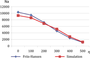
Figure 11. Impact of the separation distance η - Head on collisions.

Figure 12. Impact of the separation distance η - Overtaking collisions.
The above examples confirm that the introduced simulation method can replace analytical methods very efficiently. Accordingly, it can be assumed that in other, more complex situations, the simulation model will work equally well. Furthermore, during the simulation it is possible to monitor the simulated movement of ships and points of collisions (e.g. see Figures 13, 14 and 15).

Figure 13. Comparison of collisions-traffic with normal (left) and uniform distribution (right)-3 day simulation (example based on Case 2, η = 0).

Figure 14. Simulated head-on collisions-3 days simulation (example based on Case 2, D = 3000, η = 100).

Figure 15. Simulated overtaking collisions-3 days simulation (example based on Case 2, D = 3000, η = 100).
In addition to the accurate calculation of collision candidates, graphical presentation of ship movements is the main advantage of this model. Moreover, the model should be considered as the groundwork for new advanced simulations that might include other specific situations (bend of routes, groundings, dangers on route, etc.), as well as different distributions of ship traffic, change in traffic volume over time intervals, influence of external factors (currents, winds…), human errors, more realistic ship movements in a parallel courses, etc.
6. CONCLUSIONS
Calculation of the potential number of collision candidates is a widely accepted method in the prediction of accidents, primarily due to the possibility of taking into account various characteristics of the traffic flows. Besides the positive aspects of this approach, there are also certain shortcomings. The main problem is the unknown causation probability, which is generally unique for each area, and is as such required in order to obtain the absolute number of collisions. Despite this, usefulness of calculating the potential number of collisions is undisputable, especially when comparing two or more similar sailing routes.It is possible to use various analytical methods and simulations in order to obtain the potential number of collisions. Both approaches produce similar results, regarding the total number of collisions and the changes of these values in different route crossing scenarios.The simulation model, as introduced in this paper, may take more time to run as it requires more repetitions, but its main advantage is the ability to show ship movements and potential collision points in overlapping areas, using a user-friendly interface and graphic animation. Also, this simulation model confirms that it is possible to simplify the programming process by replacing the actual vessels and their characteristics by geometric circles. Accordingly, further development of more complex simulations can be based on the same principle, e.g. expansion of the simulation by taking into account additional external and internal factors that affect the movement of ships, especially hydrographic impacts and human errors. The model can be also expanded in order to simulate other scenarios such as bend of routes, groundings, etc. The presented simulation model and examples still require causation probability to obtain the real number of collisions but, as mentioned before, the model should be considered as the groundwork for new advanced simulations that might simulate, ultimately, the real movement of ships and calculate the real number of collisions (accidents).


