


1 Introduction
The rise of deep learning has been accompanied by a paradigm shift in machine learning and intelligent systems. In Natural Language Processing applications, this has been expressed via the success of distributed representations (Hinton et al. Reference Hinton, McClelland and Rumelhart1984) for text data on machine learning tasks. These typically come in the form of text embeddings, which are vector space representations able to capture features beyond simple statistical properties, Such approaches try to evolve over the histogram-based accumulation used in methods like the bag-of-words model (Salton and Buckley Reference Salton and Buckley1988). Instead of applying a handcrafted rule, text embeddings learn a transformation of the elements in the input. This approach avoids the common problem of extreme feature sparsity and mitigates the curse of dimensionality that usually plagues shallow representations.
There have been numerous approaches to learning text embeddings. Early attempts produce shallow vector space features to represent text elements, such as words and documents, via histogram-based methods (Katz Reference Katz1987; Salton and Buckley Reference Salton and Buckley1988; Joachims Reference Joachims1998). Other approaches use topic modeling techniques, such as Latent Semantic Indexing (Deerwester et al. Reference Deerwester, Dumais, Furnas, Landauer and Harshman1990) and Latent Dirichlet Allocation (Hingmire et al. Reference Hingmire, Chougule, Palshikar and Chakraborti2013). In these cases, latent topics are inferred to form a new, efficient representation space for text. Regarding neural approaches, a neural language model applied on word sequences is used in Bengio et al. (Reference Bengio, Ducharme, Vincent and Jauvin2003) to jointly learn word embeddings and the probability function of the input word collection. Later approaches utilize convolutional deep networks, such as the unified multitask network in Collobert and Weston (Reference Collobert and Weston2008), or introduce recurrent neural networks, as in Mikolov et al. (Reference Mikolov, Kombrink, Burget, Cernocký and Khudanpur2011). Deep neural models are used to learn semantically aware embeddings between words (Mikolov et al. Reference Mikolov, Karafiát, Burget, Cernocký and Khudanpur2010; Reference Mikolov, Kombrink, Burget, Cernocký and Khudanpur2011). These embeddings try to maintain semantic relatedness between concepts, but also support meaningful algebraic operators between them. The popular word2vec embeddings (Mikolov et al. Reference Mikolov, Chen, Corrado and Dean2013a) learn such embedding spaces via Continuous Bag-Of-Words (CBOW) or skip-gram patterns, sometimes varying the context sampling approach (Mikolov et al. Reference Mikolov, Sutskever, Chen, Corrado and Dean2013b).
Despite numerous successful applications of text embeddings, most approaches largely ignore the rich semantic information that is often associated with the input data. Typically, such information, for example, in the form of knowledge bases and semantic graphs, is readily available from human experts. This fact can function both as an advantage and a disadvantage in learning tasks. On the one hand, if the learned model is not restricted by human experts’ rules and biases, it is free to discover potentially different (and often superior) intermediate representations of the input data (Bengio et al. Reference Bengio2009) for a given task. On the other hand, ignoring the wealth of existing information means that any useful attribute is captured by relearning from scratch, a process that requires large amounts of training resources.
We claim that we need to investigate hybrid methods, combining the best of both worlds. As such, these methods will allow a model to search the feature space for optimal representations, while being able to exploit preexisting expert features. We expect such a paradigm shift to affect a multitude of Natural Language Processing tasks, from classification to clustering and summarization. Furthermore, it allows researchers to utilize a full range of different structure over resources: raw text, documents accompanied by metadata and multimodal components (e.g., embedded images, audio). However, we expect that the way of introducing semantic information to the model will affect training and the performance of the learned model on the task at hand.
In this context, this work suggests a method to integrate semantic information into a neural classification pipeline and evaluates the outcome. We model the pipeline as a hybrid, branched architecture (cf. Figure 1), where each branch corresponds to one aspect of the hybrid: semantically driven versus raw-data-driven.
Given an input text, the semantically driven branch, elaborated in Section 3, does the following:
-
• For each word, it extracts semantic information from an appropriate resource of existing knowledge, such as a semantic graph.
-
• It generates a semantic vector for the word.
-
• It represents the whole text as a fusion of the word semantic vectors.
The raw-data-driven branch utilizes raw data information to generate a word embedding as we find in many deep learning-related works. Finally, we augment the word embedding output representations by the semantic vector, feeding the resulting enriched, hybrid representation to a deep neural network (DNN) classifier.
Based on this formulation, we address the following research questions in the context of the single-label text classification task:
-
1. Can semantic information increase the task performance, when applied in this setting? If so, how much?
-
2. How much do the different semantic disambiguation methods affect the above performance increase?
-
3. What is the effect of taking into account hypernymy relations in the semantic branch of the representation?
The rest of the paper is structured as follows. Section 2 surveys relevant works on semantic augmentation methods for classification problems, as well as the main techniques for enriching word embeddings with semantic information. In Section 3, we elaborate on our method, describing (a) the embeddings generation, (b) the semantic information extraction, and (c) the vector augmentation steps. Section 4 presents the experimental study that evaluates the performance of our workflow and compares it to the state of the art in the field. It also addressing the above three research questions based on the results. We conclude the paper with a summary of our key findings along with directions for future work in Section 5.
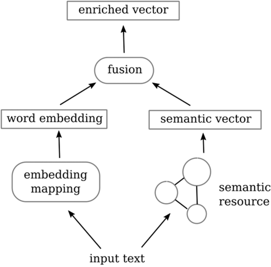
Figure 1. Overview of our approach to semantically augmenting the classifier input vector.
2 Related work
In this study, we explore the introduction of semantic information into text-based embeddings, in the context of single-label text classification. Given a collection of text documents
 $T=\{t_1, \dots, t_N\}$
, a set of c predefined labels
$T=\{t_1, \dots, t_N\}$
, a set of c predefined labels
 $L=\{l_1, \dots, l_c\},$
and existing document-to-label annotations
$L=\{l_1, \dots, l_c\},$
and existing document-to-label annotations
 $G = \{(t_1, g_1), \dots, (t_N, g_N)\}, g_i \in L$
such that the label of document
$G = \{(t_1, g_1), \dots, (t_N, g_N)\}, g_i \in L$
such that the label of document
 $t_i$
is
$t_i$
is
 $g_i$
, the task is to find a classification function f that produces the correct label for each input document, that is,
$g_i$
, the task is to find a classification function f that produces the correct label for each input document, that is,
 $f(t_i) = g_{i}$
.
$f(t_i) = g_{i}$
.
Specifically, we focus on DNN classifiers in conjunction with word embeddings for representing and feeding the input text to the predictive model.
In the literature, numerous studies leverage semantic knowledge to augment text mining tasks. For classification, graph-based semantic resources such as the WordNet ontology (Miller Reference Miller1995) have been widely used to enrich textual information. Early approaches examined the effect of WordNet’s semantic information on binary text classification, using rule-based discrimination (Scott and Matwin Reference Scott and Matwin1998) as well as support vector machine (SVM) classification (Mansuy and Hilderman Reference Mansuy and Hilderman2006). In Elberrichi, Rahmoun, and Bentaalah (Reference Elberrichi, Rahmoun and Bentaalah2008), the bag-of-words vector representation (Salton and Buckley Reference Salton and Buckley1988) is combined with the WordNet semantic graph. A variety of semantic selection and combination strategies are explored, along with a supervised feature selection phase that is based on the chi-squared statistic. The experimental evaluation on the 20-Newsgroups and Reuters datasets shows that the semantic augmentation aids classification, especially when considering the most frequent related concept of a word. Frequency-based approaches are examined in Nezreg, Lehbab, and Belbachir (Reference Nezreg, Lehbab and Belbachir2014) over the same two datasets, applying multiple classifiers to terms, WordNet concepts and their combination. The combined approach yields the best results for both datasets; however, (a) it uses handcrafted features for the representation of textual information and (b) it employs shallow methods for classification, and (c) it considers subsets of the two datasets.
On another line of research, neural methods are coupled with relationships from the WordNet semantic graph (Morin and Bengio Reference Morin and Bengio2005), producing a language model where words are represented in a binary tree via hierarchical clustering—rather than deriving such a hierarchy from training data. The resulting model trains faster and performs better than the bag-of-words baselines, but worse than the neural language model of Bengio et al. (Reference Bengio, Ducharme, Vincent and Jauvin2003).
A bulk of later works modify the deep neural embedding training, with many of them investigating ways of introducing both distributional and relational information into word embeddings. Distributional information pertain to statistics from the context of a word, while relational information utilizes semantic relationships such as synonymy and hypernymy.
In more detail, the “retrofitting” method is used in Faruqui et al. (Reference Faruqui, Dodge, Jauhar, Dyer, Hovy and Smith2015) to shift word embeddings toward points in the embedding space that are more suitable to represent semantic relationships within an undirected graph. This is accomplished by post-processing the existing word vectors to balance their distance between their original fitted values and their semantic neighbors. The experimental analysis demonstrates the resulting improvements on the embeddings in a multilingual setting, with respect to a variety of semantic-content tasks. The retrofitting system is specialized in Glavaš and Vulić (Reference Glavaš and Vulić2018) via a feed-forward DNN that explicitly maps semantic/relational constraints into modified training instances to produce specialized embeddings. The authors report significant gains in a series of tasks that range from word similarity to lexical simplification and dialog state tracking. The study in Yu and Dredze (Reference Yu and Dredze2014) extends the neural language model of Bengio et al. (Reference Bengio, Ducharme, Vincent and Jauvin2003) and Mikolov et al. (Reference Mikolov, Karafiát, Burget, Cernocký and Khudanpur2010) with semantic priors from WordNet and Paraphrase (Ganitkevitch, Van Durme, and Callison-Burch Reference Ganitkevitch, Van Durme and Callison-Burch2013). Their “Relation Constrained Model” (RCM) modifies the CBOW (Mikolov et al. Reference Mikolov, Sutskever, Chen, Corrado and Dean2013b) algorithm, by modifying the objective function to consider only word pairs joined by a relation defined in the semantic ground truth. Additionally, they explore a joint model where the objective function considers a weighted linear combination of both corpus co-occurrence statistics and relatedness based on the knowledge resource. An experimental evaluation on language modeling, semantic similarity, and human judgment prediction over a subset of the Gigaword corpus (Parker et al. Reference Parker, Graff, Kong, Chen and Maeda2011) demonstrates that using the joint model for pre-training RCM results in the largest performance increase, with respect to standard word2vec embeddings.
In Fried and Duh (Reference Fried and Duh2014), the authors model semantic relatedness by computing the length of the shortest path between WordNet synsets. This is mapped to a word pair by considering the maximum possible distance between candidate synset pairs associated with these words. A scaled version of this length regularizes the cosine similarity of the word pair corresponding word embeddings. Both distributional and semantic information are jointly trained via the ADMM multi-objective optimization approach (Boyd et al. Reference Boyd, Parikh, Chu, Peleato and Eckstein2011). The authors evaluate their graph distance measure—along with other WordNet distance approaches—on multiple tasks, such as knowledge base completion, relational similarity, and dependency parsing. The overall results indicate that utilizing semantic resources provide a performance advantage, compared to using text-only methods.
In Vulic and Mrkšic (Reference Vulic and Mrkšic2018), embeddings are fine-tuned to respect the WordNet hypernymy hierarchy, and a novel asymmetric similarity measure is proposed for comparing such representations. This results in state-of-the-art performance on multiple lexical entailment tasks.
Furthermore, the authors in Xu et al. (Reference Xu, Bai, Bian, Gao, Wang, Liu and Liu2014) use skip-grams with relational, categorical as well as joint semantic biases in the objective function. To achieve this, they model a relation r between entities a and b as vector translation (e.g.,
 $a + r = b$
), that is, modeling both entities and relations in the same vector space. Categorical knowledge is limited to fine-grained similarity scores, after discarding too generic entity relationships. All variants are evaluated on analogical reasoning, word similarity, and topic prediction tasks, with the experimental results demonstrating that the joint model outperforms its single-channel counterparts (the semantically aware networks and baseline skip-gram embeddings). In Bian, Gao, and Liu (Reference Bian, Gao and Liu2014), the authors use external resources to introduce syntactic, morphological, and semantic information into the generation of embeddings. Experimental results on analogical reasoning and word similarity sentence completion show that the semantic augmentation is the most reliable augmentation approach, compared to a CBOW baseline, with the other resources producing inconsistent effects on performance. The approach in Luong, Socher, and Manning (Reference Luong, Socher and Manning2013) exploits morphological characteristics by training a recursive neural network at the level of a morpheme, rather than a word, which allows for generating embeddings for unseen words on-the-fly. The authors report large gains on the word similarity task across several datasets. Other approaches to fine-tuning embeddings seek to produce robust feature vectors with respect to language characteristics (Ruder, Vulić, and Søgaard Reference Ruder, Vulić and Søgaard2019), instead of enforcing explicit semantic relationships.
$a + r = b$
), that is, modeling both entities and relations in the same vector space. Categorical knowledge is limited to fine-grained similarity scores, after discarding too generic entity relationships. All variants are evaluated on analogical reasoning, word similarity, and topic prediction tasks, with the experimental results demonstrating that the joint model outperforms its single-channel counterparts (the semantically aware networks and baseline skip-gram embeddings). In Bian, Gao, and Liu (Reference Bian, Gao and Liu2014), the authors use external resources to introduce syntactic, morphological, and semantic information into the generation of embeddings. Experimental results on analogical reasoning and word similarity sentence completion show that the semantic augmentation is the most reliable augmentation approach, compared to a CBOW baseline, with the other resources producing inconsistent effects on performance. The approach in Luong, Socher, and Manning (Reference Luong, Socher and Manning2013) exploits morphological characteristics by training a recursive neural network at the level of a morpheme, rather than a word, which allows for generating embeddings for unseen words on-the-fly. The authors report large gains on the word similarity task across several datasets. Other approaches to fine-tuning embeddings seek to produce robust feature vectors with respect to language characteristics (Ruder, Vulić, and Søgaard Reference Ruder, Vulić and Søgaard2019), instead of enforcing explicit semantic relationships.
Some approaches apply their findings on text and/or document classification. The authors in Card, Tan, and Smith (Reference Card, Tan and Smith2018) propose a neural topic modeling framework that is able to incorporate metadata such as annotations/tags as well as document “covariates” (e.g., year of publication), with tunable performance trade-offs. Experiments over a US immigration dataset show that this approach outperforms supervised latent dirichlet allocation (LDA) (Mcauliffe and Blei Reference Mcauliffe and Blei2008) on document classification. In Li et al. (Reference Li, Wei, Yao, Chen and Li2017), the authors use a document-level embedding that is based on word2vec and concepts mined from knowledge bases. They evaluate their method on dataset splits from 20-Newsgroups and Reuters-21578, but this evaluation uses limited versions of the original datasets.
To tackle word polysemy and under/misrepresentations of semantic relationships in the training text, many approaches build embeddings for semantic concepts (or “senses”), instead of words. Such “sense embedding” vectors are studied in Chen, Liu, and Sun (Reference Chen, Liu and Sun2014), where the authors emphasize the weaknesses of distributional, cluster-based models like the ones in Huang et al. (Reference Huang, Socher, Manning and Ng2012). Instead, they use skip-gram initialized word embeddings, aggregated to sense-level vectors by combining synset definition word vectors from WordNet. Word sense disambiguation (WSD) is performed via a context vector, with strategies based on word order or candidate sense set size, for each ambiguous word. Learning uses the skip-gram objective imbued with sense prediction. Evaluations on domain-specific data (i.e., small portion of the Reuters corpus) for coarse-grained semantic disambiguation (corresponding SemEval 2007 task Navigli, Litkowski, and Hargraves Reference Navigli, Litkowski and Hargraves2007) show that the proposed model performs similar to or above the state of the art, with the authors stressing the reusability of their approach.
In Iacobacci, Pilehvar, and Navigli (Reference Iacobacci, Pilehvar and Navigli2015), the authors introduce “Sensembed”, a framework that generates both semantic annotation tags for a given dataset and sense-level embeddings from the resulting annotated corpus. In their approach, the BabelNet semantic graph (Navigli and Ponzetto Reference Navigli and Ponzetto2012) is used to annotate a Wikipedia dump so as to create a large semantically annotated corpus via the BabelFly WSD algorithm (Moro, Raganato, and Navigli Reference Moro, Raganato and Navigli2014). Out of the disambiguated corpus, sense vectors are produced with the CBOW model (Mikolov et al. Reference Mikolov, Sutskever, Chen, Corrado and Dean2013b). These vectors are subsequently evaluated in multiple word similarity, relatedness, and word-context similarity tasks on multiple datasets. SensEmbed outperforms lexical word embeddings, as well as many related sense-based approaches on word similarity, with respect to Spearman’s correlation. It also performs better than mutual information-based baselines and word2vec embeddings on the SemEval-2012 relational similarity task (Jurgens et al. Reference Jurgens, Turney, Mohammad and Holyoak2012). SensEmbed is used in Bovi, Anke, and Navigli (Reference Bovi, Anke and Navigli2015), where the knowledge base disambiguation and unification framework “KB-UNIFY” employs sense embeddings for the disambiguation stage, along with cross-resource entity linking and alignment, so as to unify and merge semantic resources. In Flekova and Gurevych (Reference Flekova and Gurevych2016), the authors employ WordNet supersenses, that is, flat groupings of synsets, denoting synset high-level and more abstract semantic information that regular WordNet entities. BabelNet synsets are mapped to WordNet supersenses, using an automatically annotated Wikipedia corpus at multiple abstraction levels (Scozzafava et al. Reference Scozzafava, Raganato, Moro and Navigli2015). A range of evaluations on downstream classification tasks (subjectivity, metaphor, and polarity classification) demonstrates that the proposed approach yields state-of-the art results, outperforming the exclusive use of distributional information. Further, the “AutoExtend” method (Rothe and Schütze Reference Rothe and Schütze2015) uses WordNet, considering words and synsets as a sum of their lexemes. Word embeddings are learned (or existing ones are modified) by a deep autoencoder, with the hidden layers representing synset vectors. Experiments on WSD, using the SensEval task corpora, show that AutoExtend achieves higher accuracy than an SVM-based approach with multiple engineered semantic features, with a subsequent combination of the two approaches further improving performance—indicating complementarity between them. In addition, an evaluation on word similarity shows that AutoExtend outperforms other systems (Huang et al. Reference Huang, Socher, Manning and Ng2012; Mikolov et al. Reference Mikolov, Sutskever, Chen, Corrado and Dean2013b; Chen et al. Reference Chen, Liu and Sun2014) as well as synset-level embeddings, in terms of Spearman’s correlation. In Goikoetxea, Agirre, and Soroa (Reference Goikoetxea, Agirre and Soroa2016), semantic embeddings are computed independently: a probabilistic random walk over the semantic graph outputs sequences of synsets, with the latter mapped to words via a dictionary of WordNet gloss relations. The resulting pseudo-corpus is fed to the skip-gram algorithm to learn semantic embeddings. Lexical and semantic vectors are subsequently combined in various ways, with simple concatenation outperforming more sophisticated semantic augmentation methods, such as retrofitting, on similarity and relatedness datasets and tasks.
The approach in Pilehvar et al. (Reference Pilehvar, Camacho-Collados, Navigli and Collier2017) examines the effect of sense and supersense information on text classification and polarity detection tasks. Disambiguation is performed by mapping the input sentence into a subgraph of the semantic resource containing all semantic candidates per word. Then, the sense with the highest node degree is picked for each word, discarding the rest and pruning the subgraph accordingly. Additionally, supersenses are produced via averaging synset vectors with respect to the grouping of senses provided in WordNet lexicographer files. An experimental evaluation over the BBC, 20-Newsgroups, and Ohsumed datasets shows that their approach introduces significant benefits in terms of F1-score, consistently improving the lexical embedding baseline on randomly initialized vectors. However, no improvement is observed when using pre-trained embeddings. For polarity detection, no consistent improvement is reported either. This is attributed to the short document sizes and the lack of word ambiguity in the examined datasets.
These approaches effectively introduce semantic information to deep neural architectures and word embeddings, but the evaluation of the refined embeddings on applied machine learning scenarios is limited, focusing for the most part on a variety of semantic similarity tasks or specialized domain-specific classification tasks. Instead, this study focuses on a specific machine learning task, namely text classification, exploring the effect of semantic augmentation on deep neural models to the classification performance. Our worked is focused on the feature level, applying semantic enrichment on the input space of the classification process. We separate the embedding generation from the semantic enrichment phase, as in Faruqui et al. (Reference Faruqui, Dodge, Jauhar, Dyer, Hovy and Smith2015), where the semantic augmentation can be applied as a post-processing step. In fact, we model the semantic content as a separate representation of the input data that can be combined with a variety of embeddings, features, and classifiers. Our approach extends earlier work on shallow features and learners (Scott and Matwin Reference Scott and Matwin1998; Mansuy and Hilderman Reference Mansuy and Hilderman2006; Elberrichi et al. Reference Elberrichi, Rahmoun and Bentaalah2008; Nezreg et al. Reference Nezreg, Lehbab and Belbachir2014) by augmenting deep embedding generators instead of local features. We also expand our investigation to additional semantic extraction and disambiguation approaches, by considering the effect of the n-th degree hypernymy relations and of several context semantic embedding methods. Finally, we expand and complement the findings of Pilehvar et al. (Reference Pilehvar, Camacho-Collados, Navigli and Collier2017), adopting multiple disambiguation schemes and a comparatively lower complexity architecture for classification.
3 Approach
We now delve into our approach for introducing external semantic information into the neural model. We present the textual (raw text) component of our learning pipeline in Section 3.1, the semantic component in Section 3.2, and the training process that builds the classification model in Section 3.3.
3.1 Text preprocessing and embedding generation
We begin by applying preprocessing to each document in order to discard noise and superfluous elements that are deemed irrelevant or even harmful for the task at hand. The processing tokenizes the original texts into a list of words and discards non-lexical elements, such as punctuation, whitespace, and stopwords.Footnote a To generate word embeddings, we employ the established word2vec algorithm (Mikolov et al. Reference Mikolov, Sutskever, Chen, Corrado and Dean2013b). Specifically, we use the CBOW variant for the training process, which produces word vector representations by modeling co-occurrence statistics of each word based on its surrounding context. Instead of using pre-trained embeddings, we extract them from the given corpus, using a context window size of 10 words. To discard outliers, we also apply a filtering phase, which discards words that fail to appear at least twice in the training data. We train the embedding representation over 50 epochs (i.e., iterations over the corpus), producing 50-dimensional vector representations for each word in the resulting dataset vocabulary. These embeddings represent the textual/lexical information of our classification pipeline.
3.2 Semantic enrichment
We now elaborate on the core of our approach, which infuses the trained embeddings with semantic information. First, we describe the semantic resource we use, WordNet. Then we introduce the semantic disambiguation phase which, given a word, selects a single element from a list of WordNet concepts as appropriate for the word. We continue with a description of the propagation mechanism we apply to spread semantic activation, that is to include more semantic information related to the concept in the word representation. We conclude with the fusion strategy by which we combine all information channels to a single enriched representation.
3.2.1 Semantic resource
We use WordNet (Miller Reference Miller1995),Footnote b a popular lexical database for the English language that is widely used in classification and clustering tasks (Hung and Wermter Reference Hung and Wermter2004; Morin and Bengio Reference Morin and Bengio2005; Liu et al. Reference Liu, Scheuermann, Li and Zhu2007; Elberrichi et al. Reference Elberrichi, Rahmoun and Bentaalah2008). WordNet consists of a graph, where each node is a set of word senses (called synonymous sets or synsets) representing the same approximate meaning, with each sense also conveying part-of-speech (POS) information.
Synset nodes are connected to neighbors through a variety of relations of lexical and semantic nature (e.g., is-a relations like hypernymy and hyponymy, part-of relations such as meronymy, and others). Note that while the terms “synset” and “concept” are similar enough to merit interchangeable use, we will use the word “concept” throughout the paper when not talking about the internal mechanics of WordNet.
Concerning WordNet synsets, in the following paragraphs, we employ a notation inspired by Navigli (Reference Navigli2009), as follows. In WordNet, the graph node encapsulating the everyday concept of a dog is a synset s, composed of individual word senses of near-identical semantic content, as below:
 \begin{equation} \nonumber s = \left\{ dog_n^1, domestic\_dog_n^1, Canis\_familiaris_n^1 \right\}\end{equation}
The subscript of each word sense denotes POS information (e.g., nouns, in this example), while the superscript denotes a sense numeric identifier, differentiating between-individual word senses. Given a word sense, we can unambiguously identify the corresponding synset, enabling us to resolve potential ambiguity (Martin and Jurafsky Reference Martin and Jurafsky2009; Navigli Reference Navigli2009) of polysemous words. Thus, in the following paragraphs, we will use the notation
 $l.p.i$
to refer to the synset that contains the i-th word sense of the lexicalization l that is of a POS p.
$l.p.i$
to refer to the synset that contains the i-th word sense of the lexicalization l that is of a POS p.
For example, the common meaning of the word “dog” is approximately aligned with any of the word senses in the synset s, which in WordNet is accompanied by a definition: “a member of the genus Canis (probably descended from the common wolf that has been domesticated by man since prehistoric times; occurs in many breeds”. However, additional more obscure senses of “dog” can be found in WordNet, for example,
 $dog_n^3$
, mapped to the synset defined as “informal term for a man”.Footnote c
$dog_n^3$
, mapped to the synset defined as “informal term for a man”.Footnote c
Thus, synset s will be referred to as
 $dog.n.01$
, directly pointing to the (first) word sense of the word noun “dog”.Footnote d Using this notation, we move on to describe the disambiguation process.
$dog.n.01$
, directly pointing to the (first) word sense of the word noun “dog”.Footnote d Using this notation, we move on to describe the disambiguation process.
3.2.2 Disambiguation
We extract information from WordNet via the natural language toolkit (NLTK) interface.Footnote e Its API supports the retrieval of a collection of synsets as possible semantic candidates for an input word. It also allows traversal of the WordNet graph via the synset relation links mentioned above. Below, we will denote string literals with a quoted block of text (e.g., “dog”).
To select the most relevant synset from the acquired response of the API, we employ one of the following three disambiguation strategies:
-
1. The basic disambiguation strategy serves as a baseline, simply selecting the first synset from the retrieved list, discarding the rest. The NLTK WordNet API ranks the retrieved synsets for a word query with respect to corresponding word sense frequencies computed in the SemCor sense-tagged corpus (Miller et al. Reference Miller, Leacock, Tengi and Bunker1993; Martin and Jurafsky Reference Martin and Jurafsky2009; Navigli Reference Navigli2009). Therefore, this method selects the most common meaning for the word (as computed in the SemCor text collection). An illustration of this selection process is shown in Figure 2.

Figure 2. Example of the basic disambiguation strategy. Given the list of candidate synsets from the NLTK WordNet API, the first item is selected.
-
2. The POS disambiguation strategy first filters the retrieved list of candidate synsets. The filtering discards all synsets that do not match the POS tag of the query word. Then, the first remaining synset is selected.
-
For example, when the word “can” is supplied with the POS tag “verb”, the synset defined as “airtight sealed metal container for food or drink or paint etc.” is discarded from the candidate synset list. After this filtering phase, the same mechanism as with the basic disambiguation process is applied. See Figure 3 for a visualization of this process.
Figure 3. Example of the POS disambiguation strategy. Given the candidate synsets retrieved from the NLTK WordNet API, the ones that are annotated with a POS tag that does not match the respective tag of the query word are discarded. After this filtering process, the basic selection strategy is applied.
-
3. The context-embedding disambiguation strategy uses a semantic embedding approach. For each candidate synset, related words are extracted from the accompanying example sentences together with the corresponding synset definition (i.e., the gloss).Footnote f Given the set of words from both sources, we compute the embedding mapping via the process described in Section 3.1. This associates every candidate synset with the set of embeddings of all words in its context.


To arrive at a single vector representation for every candidate synset, this strategy averages all components across word embeddings in the context. This process maps the semantic information into a shared representation with the lexical/textual one. In other words, it projects synsets into the same vector space. As a result, disambiguation by vector comparison is enabled: given a word w, its embedding
 $e_w$
, and a set of synset embeddings
$e_w$
, and a set of synset embeddings
 $S = \{e_1, \dots, e_{|S|}\}$
, we assign w to the synset
$S = \{e_1, \dots, e_{|S|}\}$
, we assign w to the synset
 ${s = \underset{S}{argmin}\left[ dist(e_w, e_s) \right]}$
, where
${s = \underset{S}{argmin}\left[ dist(e_w, e_s) \right]}$
, where
 $e_s$
is the aggregated synset embedding for synset
$e_s$
is the aggregated synset embedding for synset
 $s \in S$
and
$s \in S$
and
 $dist(\cdot, \cdot)$
denotes a vector distance metric.
$dist(\cdot, \cdot)$
denotes a vector distance metric.
To ensure adequate word context for generating representative semantic embeddings, we discard all synsets with fewer than 25 context words. The synset vector computation process from the whole WordNet, which is illustrated in Figure 4, results in 753 adequately represented synsets. The disambiguation process itself is depicted in Figure 5.
Overall, the context-embedding disambiguation strategy performs synset selection in a significantly more complicated manner than the other two strategies. Rather than using low-level lexical information (basic strategy) or lexical and syntactic features (POS strategy), this approach exploits the available distributional information in WordNet in order to match the input word to a synset.

Figure 4. Example of the synset vector generation for context-embedding disambiguation strategy. The context of each synset is tokenized into words, with each word mapped to a vector representation via the learned embedding matrix. The synset vector is the centroid produced by averaging all context word embeddings.

Figure 5. Example of the disambiguation phase of the context-embedding disambiguation strategy. A candidate word is mapped to its embedding representation and compared to the list of available synset vectors. The synset with the vector representation closest to the word embedding is selected.
This strategy bears some resemblance to other embedding-based disambiguation methods in the literature. However, given (a) the paper’s focus on the downstream task of classification and (b) the multiple other disambiguation strategies examined, we decided to build a straightforward approach as described above; this way, we managed to reduce both the number of decision points (thus largely avoiding heuristics engineering and metaparameter optimization) as well as the computational requirements of this embedding-based disambiguation approach, in favor of a more robust, readily applicable algorithm. Comparatively, an example of a similar embedding-based approach is the work in Chen et al. (Reference Chen, Liu and Sun2014), where the authors build synset embeddings via a process that includes averaging vectors of words that are related to WordNet synsets. However, their method is considerably more intricate compared to ours, since in their approach (i) semantic vectors are additionally fitted, with the aforementioned scheme being used just for sense vector initialization, (ii) a filtering step is used to process the WordNet gloss text prior to vector initialization, using a predefined subset of POS tags, and (iii) only words with representations close to the candidate word in a embedding space are considered, using a distance/similarity threshold. In contrast, context-embedding directly pools all available textual resources that accompany a synset in order to construct an embedding, that is, utilizing all available distributional information WordNet has to offer. Additionally, no further fitting is applied to the resulting embedding, but it is used as-is in the downstream classification task for disambiguation purposes (i.e., to retrieve the synset that will be used in the actual semantic information extraction component).
3.2.3 n-level hypernymy propagation
Since WordNet represents a graph of interconnected synsets, we can exploit meaningful semantic connections to activate relevant neighboring synsets among the candidate ones. In fact, our approach propagates activations further than the immediate neighbors of the retrieved candidate synsets, to a multistep, n-level relation set. This way, a spreading activation step (Collins and Loftus Reference Collins and Loftus1975) propagates the semantic synset activation toward synsets connected with hypernymy relations with the initial match. In other words, it follows the edges labeled with is-a relations to include the encountered synsets in the pool of retrieved synsets.
The synsets extracted with this process are annotated with weights inversely proportional to the distance of the hypernymy level from the original synset. This weight decay is applied to diminish the contribution of general and/or abstract synsets, which are expected to be encountered frequently, thus saturating the final semantic vector.
After a hyper-parameter tuning phase, we arrived at the configuration of a three-level propagation process, with each level associated with a weight decay factor of 0.6. This mechanism enables words to share semantic information even if they do not belong to the same synset directly, but their mapped synsets can be linked via a short walk in the semantic graph—the longer the path, the lower the resulting relatedness weight.
To illustrate the spreading activation mechanism, consider querying the NLTK WordNet interface with the input word “dog” as an example. Using the basic disambiguation strategy (cf. Section 3.2.2), the first synset is selected out of the retrieved list, i.e., it is the synset
 $dog.n.01 = \left\{ dog_n^1, domestic\_dog_n^1, Canis\_familiaris_n^1 \right\}$
and is valued with a unit weight. Subsequently, our spreading activation procedure is activated and operates as follows:
$dog.n.01 = \left\{ dog_n^1, domestic\_dog_n^1, Canis\_familiaris_n^1 \right\}$
and is valued with a unit weight. Subsequently, our spreading activation procedure is activated and operates as follows:
-
– The first step yields the direct hypernyms of the synset
$dog.n.01$
in the WordNet graph:
$h_1 = \{x \vert dog.n.01 \text{ is-a } x\} = \{{canine.n.02}, {domestic\_animal.n.01}\}$
, with
${canine}= \left\{ canine_n^2, canid_n^2 \right\}$
and
${domestic\_animal.n.01} = \{domestic\_animal_n^1, domesticated\_animal_n^1\}$
. These two synsets are thus assigned a weight of
$0.6^{1}=0.6$
. -
– Next, we retrieve the hypernyms of each synset in
$h_1$
. This yields the synsets
$h_2=\{carnivore.n.01, animal.n.01\}$
, each weighted with
$0.6^{2} = 0.36$
. -
– Finally, the third step produces the synsets
$h_3 = \{placental.n.01, organism.n.01\}$
, each with a weight of
$0.6^{3} = 0.216$
.


As a result, the result of the three-level spreading activation procedure on the word “dog” is a semantic vector with values:
 $[1, 0.6, 0.6, 0.36, 0.36, 0.216, 0.216]$
corresponding to weights for the synsets
$[1, 0.6, 0.6, 0.36, 0.36, 0.216, 0.216]$
corresponding to weights for the synsets
 $[dog.n.01, canine.n.02, domestic\_animal.n.01,$
 $carnivore.n.01, animal.n.01, placental.n.01, organism.n.01]$
. This example is also illustrated in Figure 6. Having this mapping of word to name-value collections, the next section describes the procedure by which the word-level information is fused to arrive at document-level vectors.
$carnivore.n.01, animal.n.01, placental.n.01, organism.n.01]$
. This example is also illustrated in Figure 6. Having this mapping of word to name-value collections, the next section describes the procedure by which the word-level information is fused to arrive at document-level vectors.
3.2.4 Fusion
As explained above, each semantic extraction process yields a set of concept-weight pairs for each word in the document. We want a single, constant length, semantic vector for each document. Thus, we form this vector by following a bag-of-synsets/concepts approach: we create a vector space where each dimension is mapped to one of the concepts discovered in the corpus; then we apply the semantic extraction to all documents in the corpus, mapping each of these documents in the space based on the frequency of a concept in the document. Thus, similar to the bag-of-word paradigms, we can generate two different vector types:
-
1. We consider the raw concept frequencies over each document, arriving at semantic vectors of the form
$s^{(i)} = \{s_1, s_2, \dots, s_d\}$
, where
$s^{(i)}_j$
denotes the frequency of the j-th concept in the i-th document. A concept in the semantic vector appears at least once in the training dataset. Note that concepts extracted from the test dataset, which do not appear in the training dataset, are discarded. -
2. We apply a weighting scheme similar to TF-IDF (Salton and Buckley Reference Salton and Buckley1988) at the document and corpus levels, that is, by normalizing the document-level concept frequencies with the corresponding corpus-level frequencies:
$w^{(i)}_j = s^{(i)}_j / \Sigma_{k \in [0, \dots N]}s^{(k)}_j $
, where
$s^{(i)}_j$
stands for the raw frequency of the j-th concept in the i-th document, N is the number of documents in the dataset, and
$w^{(i)}$
is the final TF-IDF concept weight in the i-th document. This process reduces the importance of concepts that appear in too many documents in the corpus, similar to weight discounting of common words in a text retrieval setting.
Figure 6. Example of the spreading activation process for the input word “dog”, executed for three levels with a decay factor of 0.6. The solid line (a) denotes the semantic disambiguation phase with one of the covered strategies. Dashed lines ((b) through (d)) represent the extraction of synsets linked with a hypernymy (is-a) relation to any synset in the source list. The numeric values represent the weight associated with synsets of each level, with the final semantic vector for the input word being listed to the right.


After this post-processing stage, we are ready to incorporate the semantic vector into the classification pipeline. This is done in two ways:
-
1. The concat fusion strategy concatenates the embedding with the semantic vector, arriving at a semantically augmented representation that is fed to the downstream classifier.
-
2. The replace fusion strategy discards completely the lexical embedding, using only the semantic information for tackling the categorization task.
Since all cases above use semantic features that represent explicit concept-weight information (rather than explicitly distributed vectors), we do not fine-tune the augmented embeddings during training but keep the entire representation “frozen” to the original input values.
3.3 Training
We use a DNN with 2 hidden layers, each containing 512 neurons. We arrived at this configuration after fine-tuning these two hyper-parameters through a grid search on a range of values: from 1 to 4 with a step of 1 for the number of hidden layers; values of
 $\{128, 256 \dots, 2048\}$
for the number of neurons within each hidden layer. We use dropout with a heuristically selected 0.3 drop probability and position it after each dense layer to avoid overfitting. We train the DNN for 50 epochs over the total training data, with a 25-epoch early stopping, which allows the training to end prematurely, if the validation loss does not decrease for 25 consecutive epochs. We apply a fivefold cross-validation split for training and classifying the input via a softmax layer. The learning rate is initialized to 0.1, applying a reduction schedule of a 0.1 decay factor every 10 epochs on loss stagnation.
$\{128, 256 \dots, 2048\}$
for the number of neurons within each hidden layer. We use dropout with a heuristically selected 0.3 drop probability and position it after each dense layer to avoid overfitting. We train the DNN for 50 epochs over the total training data, with a 25-epoch early stopping, which allows the training to end prematurely, if the validation loss does not decrease for 25 consecutive epochs. We apply a fivefold cross-validation split for training and classifying the input via a softmax layer. The learning rate is initialized to 0.1, applying a reduction schedule of a 0.1 decay factor every 10 epochs on loss stagnation.
3.4 Workflow summary
At this point, we summarize the complete workflow of our approach to put everything we have described together, under a common view:
-
1. Preprocessing transforms each document into a sequence of informative words.
-
2. word2vec word embeddings are learned from scratch on these word sequences.
-
3. Semantic information for each document is extracted via the NLTK WordNet interface in the form of frequency-based concept vectors. This entails
-
(a) concept extraction for each word by one of the disambiguation strategies (basic, POS or context-embedding).
-
(b) three-level hypernymy activation propagation based on the WordNet graph.
-
(c) raw frequency or TF-IDF weighting.
-
-
4. The semantic information from Step 3 is combined with the word embeddings from Step 2 through a fusion strategy (concat or replace).
-
5. Classification with a DNN classifier.
The above workflow is illustrated in Figure 7.
4 Experimental evaluation
In this section, we outline the experiments performed to evaluate our semantic augmentation approaches for text classification. In Section 4.1, we describe the datasets and the experimental setup, in Section 4.2, we present and discuss the obtained results, and in Section 4.3, we compare our approach to related studies.

Figure 7. An example of the semantic augmentation process leading up to classification with a DNN classifier. The image depicts the case of concat fusion, that is, the concatenation of the word embedding with the semantic vector. The dashed box is repeated for each word in the document. Green/red colors denote semantic/textual information, respectively.
4.1 Datasets and experimental setup
We use the 20-Newsgroups dataset (Lang Reference Lang1995),Footnote g a popular text classification benchmark. This corpus consists of 11,314 and 7532 training and test instances of user USENET posts, spanning 20 categories (or “newsgroups”) that pertain to different discussion topics (e.g., alt.atheism, sci.space, rec.sport.hockey, comp.graphics, etc.). The number of instances per class varies from 377 to 600 for the training set, and from 251 to 399 for the test set, while the mean number of words is 191 and 172 per training and test document, respectively. We use the “bydate” version, in which the train and test samples are separated in time (i.e., the train and the test set instances are posted before and after a specific date).
Additionally, we utilize the Reuters-21578Footnote h dataset, which contains news articles that appeared on the Reuters financial newswire in 1987 and are commonly used for text classification evaluation. Using the traditional “ModApte” variant, the corpus comprises 9584 and 3744 training and test documents, respectively, with a labelset of 90 classes. The latter corresponds to categories related to financial activities, ranging from consumer products and goods (e.g., grain, oilseed, palladium) to more abstract monetary topics (e.g., money-fx, gnp, interest). The dataset is extremely imbalanced, ranging from 1 to 2877 training instances per class, and from 1 to 1087 test instances per class. The mean number of words is approximately 92, for both training and test documents. Most instances are labeled with a single class, with few of them having a multi-label annotation (up to 15 labels per instance). While hierarchical relationships exist between the classes, we do not consider them in our evaluation.
Given that we are only interested in single-label classification, we treat the dataset as a single-labeled corpus using all sample and label combinations that are available in the dataset. This results into a noisy labeling that is typical among folksonomy-based annotation (Peters and Stock Reference Peters and Stock2007). In such cases, lack of annotator agreement occurs regularly and increases the expected discrimination difficulty of the dataset, as we discard neither superfluous labels nor multi-labeled instances.
The technical details of each dataset are summarized in Table 1. Apart from sample and word count information, we additionally include (a) quantities pertaining to the POS information useful for the POS disambiguation method and (b) the amount of semantic information minable from the text. The POS annotation count and the synset/concept counts are expressed as ratios with respect to the number of words per document.
We note that no contextual or domain-specific information is employed in our experiments; reflected by the broad task handled in this work (i.e., text classification), both datasets are handled in an identical manner by every configuration examined in the experimental evaluation in the following section. This decision introduces an applicability/performance trade-off: first, the lack of special treatment enables each configuration to be readily applicable to any dataset, with the experimental evaluation better reflecting the generalization capability of the approach. This translates to a single processing pipeline for all datasets, without overengineered solutions on case-specific details. On the other hand, such a strategy may sacrifice performance gains attainable via accommodating domain or dataset-specific issues. However, we believe that demonstrating the generalization ability of the process is more important and, thus, we focus on this aspect in the experiments.
We used python with KerasFootnote i (Chollet et al. Reference Chollet2015) and TensorFlowFootnote j (Abadi et al. Reference Abadi, Barham, Chen, Chen, Davis, Dean, Devin, Ghemawat, Irving and Isard2016) to build the neural models. All experiments are reproducible via the code that is available on GitHub.Footnote k Document preprocessing was performed with Keras and NLTKFootnote l (Loper and Bird Reference Loper and Bird2002). We use WordNet version 3.0 for semantic information extraction via the interface available in NLTK.Footnote m The datasets and semantic resources were acquired via the scikit-learnFootnote n and NLTK APIs.Footnote o
Table 1. Technical characteristics of the 20-Newsgroups and Reuters datasets. Class samples refers to the range of the number of instances per class, while the last three rows report mean values, with the corresponding standard deviation in parenthesis. The values in the last two rows (POS and WordNet) are expressed as ratios with respect to the number of words per document

4.2 Results
We now present the results of our experimental evaluation, discussing the performance of each method per dataset.
4.2.1 20-Newsgroups
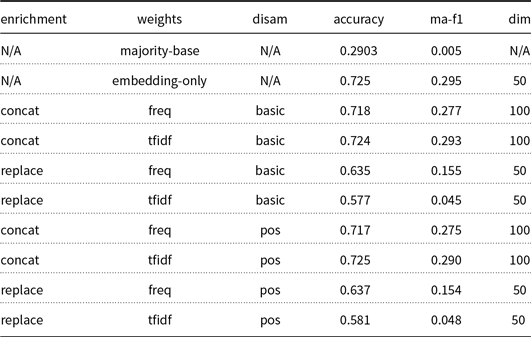
In the following tables, we present results in accuracy and macro F1-score (columns “accuracy” and “ma-f1”, respectively), in terms of mean values over five folds. We omit standard deviation scores in favor of compactness and since they consistently fall below 0.005. In the “enrichment” column, the concatenation of the embedding and the semantic vector is denoted by “concat”, whereas “replace” indicates the replacement of the former with the latter. The “features” column reports the use of raw concept frequencies (“freq”) or TF-IDF weights (“tfidf”). The “disam” column indicates the disambiguation strategy, that is, “basic”, “POS”, and “context” corresponding to basic, POS, and content-embedding, respectively. The “+spread” suffix denotes the use of the spreading activation that is outlined in Section 3.2.2. Finally, the dimensionality of each data vector is reported in the “dim” column. All results are obtained by training and evaluating the DNN model that is described in Section 3.3. Note that we include two baseline methods: the first row corresponds to the majority classifier, which always selects the class with the most samples in the training dataset, while the second row corresponds to word2vec embeddings, without any semantic augmentation applied in the vector (“embedding-only”).

Figure 8. (a) The diagonal-omitted confusion matrix, and (b) the label-wise performance chart for our best-performing configuration over the 20-Newsgroups dataset.
Table 2. 20-Newsgroups main experimental results. Underlined values outperform the “embedding-only” baseline method, while bold values indicate the best dataset-wise performance. Values in italics represent a performance boost achieved by the spreading activation in comparison to the identical configuration without it. “N/A” stands for non-applicable

Table 3. Misclassification cases for the best-performing configuration over the 20-Newsgroups dataset, where (a) the predicted label is semantically similar to the ground truth, (b) the test instance can be reasonably considered semantically ambiguous, given the labelset, (c) the error is related to the existence of critical named entities, or (d) the error is linked to context misidentification. True/predicted labels refer to the instance ground truth and the erroneous prediction of our model for that test instance, respectively. The listed slash-separated text segments from each instance are indicative samples believed to have had a contribution to misclassification

In Table 2, we present the experimental results for the 20-Newsgroups dataset, which give rise to the following observations:
-
• The introduction of semantic information brings gains in both accuracy and macro F1-score. The best combination concatenates raw frequency-based concept vectors to the word embeddings, with disambiguation applied according to the basic selection strategy.
-
• Regarding the concept selection method, projecting semantic vectors in the embedding vector space does not improve performance. POS filtering yields marginally inferior results than selecting the first retrieved synset from the WordNet API, which is the simplest and best-performing approach.
-
• The third-order hypernymy propagation via the spreading activation mechanism does not improve the baseline semantic augmentation in a consistent manner.
-
• Concatenating the word embedding with the semantic vector consistently outperforms the replacement of the former with the latter to a large extent.
-
• Raw concept frequencies always outperform the TF-IDF normalized weights.
Given these results and observations, we move on to an error analysis of our system by examining the performance of our best-performing configuration in more detail. To this end, Figure 8(a) illustrates the classification error via the confusion matrix for the best-performing configuration. To aid visualization, the diagonal has been removed. We observe that misclassification is approximately fairly concentrated in the first six classesFootnote p (i.e., alt.atheism, comp.graphics, comp.os.ms-windows.misc, comp.sys.ibm.pc.hardware, comp.sys.mac.hardware, and comp.windows.x), with peaks appearing at classes 15 and 16 (soc.religion.christian and talk.politics.guns, respectively). Additionally, Figure 8(b) depicts the label-wise performance for the best-performing configuration. We can see that most labels perform at an F1-score above a value of 0.6, with class 10 (rec.sport.hockey) being the easiest to handle by our classifier and class 19 (talk.religion.misc) being the most difficult.
Furthermore, Table 3 presents indicative misclassification cases selected from the erroneous prediction of our best-performing configuration. A number of patterns and explanations in these errors are identified by a manual analysis of the results, hereby outlined by selected examples. Specifically, four cases are identified ((a) through (d)). Example instances for each case are referred to by an ID (e.g., a1, a2, b1). For each instance we illustrate the true label, the wrong prediction made by our system, and indicative segments found in the instance text.
-
• First, our system often labels instances with very similar/plausible alternative annotations to the ground truth, which could be however arguably regarded as semantically valid—even by human evaluators—given the instance text. This case is presented in the table group (a)—semantically similar labels. In example a1, the label alt.atheism is applied instead of the true label talk.religion.misc, on a 20-Newsgroups instance discussing theism and the conversion of believers to/from atheism, while example a3 is misclassified to comp.sys.mac.hardware rather than sci.electronics, with the discussion in the text dealing with several computer parts.
-
• Similarly, our system deviates from the ground truth due to ambiguity and multiple distinct thematic topics in the textual content of many instances. These texts thus approach a multi-label nature with respect to the available classes. This case is reflected in group (b)—ambiguous/equivocal instances— where we list discussions that involve multiple terms and keywords connected to many classes. For example, b1 contains references to hardware but has a ground truth generally related to the Windows operating system, while b2 mentions multiple graphics file formats but the true label is the X window system. Instances b3 and b4 are mislabeled as sales-related posts from related keywords and terms (e.g., “revenue”, “business”, “for sale”), instead of classes linked to specific products and objects of discussion. Finally, text b5 features a lengthy discussion on US abortion legislation which was labeled as a political posting by our system, rather than a religious one.
-
• Further, there are cases where the content of the text is critically linked to a single or very few mentions of a named entity, that our model either disregards or the available data are not sufficient to leverage (table section (c)—critical named entity). Such cases are illustrated with examples c1 and c2, where knowledge that “Jack Morris” is a baseball player or that “VAX” is an IBM machine would be required to reach the correct conclusions.
-
• Additionally, some errors can arise due to the disambiguation method failing to produce to the correct sense, given the context. These cases are presented in group (d)—context miss. In instance d1, the system associates mentions of battery features to description of product aspects and/or bad reviews, predicting a sales-related text. In example d2, our model gives a very large weight on “The Devil Reincarnate” user handle, deducing a religion class from that very mention and undervaluing the other text terms. In d3, mentions of “disk” are likely linked to the hard disk drive mechanical component, rather than the software-centric sense in the context of operating systems, leading to a corresponding misclassification.
Cases of classification error that not included below may be harder to explain; potential causes for them could involve data outliers, classifier bias due to sample/instance size imbalances, etc.
Having performed an error analysis of our model, we assess the statistical significance of the performance improvements introduced by each semantic enrichment configuration. To this end, we present in Table 4 the pairwise t-test results of the experimental configurations presented above, with respect to the “embedding-only” baseline method. We can see that all configurations achieve significantly different results at a 5% confidence level, with most configurations also performing even more consistently differently at a 1% confidence level. Regarding the statistical significance of hypernymy propagation, we assess it by comparing its presence and absence, that is, “X+spread” rows against “X” rows. Min/max p values ranged from
 $9.97\mathrm{e}{-}06$
to
$9.97\mathrm{e}{-}06$
to
 $7.50\mathrm{e}{-}01$
for the accuracy score and from
$7.50\mathrm{e}{-}01$
for the accuracy score and from
 $1.29\mathrm{e}{-}05$
to
$1.29\mathrm{e}{-}05$
to
 $9.78\mathrm{e}{-}01$
for the macro F1-score (due to lack of space, we omit detailed results). There, statistical significance was achieved at the 5% confidence level for the majority of configurations, with many configurations (including those composed of POS concept selection, replace fusion, and TF-IDF weights) surpassing the 1% confidence level for accuracy.
$9.78\mathrm{e}{-}01$
for the macro F1-score (due to lack of space, we omit detailed results). There, statistical significance was achieved at the 5% confidence level for the majority of configurations, with many configurations (including those composed of POS concept selection, replace fusion, and TF-IDF weights) surpassing the 1% confidence level for accuracy.
Next, we examine the effect of dimensionality reduction on the performance of our semantic vectors. Table 5 reports the performance when discarding concepts with a raw concept-wise frequency of at least 20 occurrences, while Table 6 corresponds to keeping only the top 50 concepts, in terms of dataset-wise frequency, so as to match the word embedding dimension. We apply both filtering techniques on all configurations of our approach, except for hypernymy propagation and context embedding, due to space limitations. We observe the following patterns:
Table 4. 20-Newsgroups main experimental pairwise t-test results, with respect to the “embedding-only” baseline. Single- and double-starred values represent statistical significance at
 $5 \%$
and
$5 \%$
and
 $1 \%$
confidence levels, respectively
$1 \%$
confidence levels, respectively
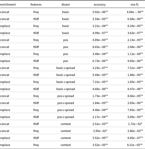
Table 5. Experiments over the 20-Newsgroups dataset for a concept-wise frequency threshold of 20. Underlined values outperform the “embedding-only” baseline

Table 6. Experiments over the 20-Newsgroups dataset for a dataset-wise frequency threshold of 50. No configuration outperforms the “embedding-only” baseline

Table 7. Reuters main experimental results. Underlined values outperform the “embedding-only” baseline, while bold values indicate the best dataset-wise performance. Values in italics denote a performance boost by the spreading activation, with respect to the identical configuration without it

-
• The frequency threshold of 20 reduces the dimensionality of the semantic vectors by more than 50%, at a minor cost in classification accuracy. Still, all configurations—excluding TF-IDF with word embedding replacement— surpass the “embedding-only” baseline. In fact, the best configuration of the main experiments (i.e., concatenation fusion with basic-selected raw frequencies) maintains a performance very close to its original one.
-
• When keeping the 50 most frequent concepts dataset-wise, only concatenation fusion is comparable to the baseline scores. For these cases, TF-IDF weights perform better than the raw concept frequencies, being very close to the baseline results. However, no configuration surpasses the baseline scores.
4.2.2 Reuters
Table 7 reports the experimental results over the Reuters-21578 dataset, which give rise to the following conclusions:
-
• We observe the same performance patterns as in the case of the 20-Newsgroups dataset. The semantic augmentation outperforms the “embedding-only” baseline, but not in all cases. The feature vectors are again high dimensional, although considerably shorter than the 20-Newsgroups dataset. This should be attributed to the fewer training documents and the significantly shorter documents (in terms of words) in the Reuters dataset.
-
• The best performance is obtained when using raw frequency features, concatenated to the word embedding with POS selection, in combination with hypernymy propagation via spreading activation. This configuration gives the best accuracy (0.749), closely followed by the same configuration with basic selection. For the macro F1-score, replacing the word embedding with frequency-based vectors, POS selection and hypernymy propagation performs the best (0.378). In fact, the replace fusion strategy holds the top three configurations with respect to macro F1-score.
-
• Regarding concept selection, the basic and the POS techniques result in very similar performance. Context embedding selection exhibits poor accuracy, performing under the “embedding-only” baseline, save for marginal improvements in macro F1-score.
-
• Spreading activation performs the best here.
-
• Comparing the replacement fusion strategy with the concatenation one almost always favors the latter, with considerable performance difference.
-
• The TF-IDF weights always perform under the raw concept frequencies, as in the 20-Newsgroups case.

Figure 9. (a) The diagonal-omitted confusion matrix and (b) the label-wise performance chart for our best-performing configuration over the Reuters dataset. For better visualization, only the 26 classes with at least 20 samples are illustrated.
Similarly to the 20-Newsgroups dataset case, we move on to the error analysis, with Figure 9(a) depicting the confusion matrix with the misclassified instances (i.e., diagonal entries are omitted). For better visualization, it illustrates only the 26 classes with at least 20 samples, due to the large number of classes in the Reuters dataset. We observe that the misclassification occurrences are more frequent, but less intense than those in the 20-Newsgroup dataset. Noticeable peaks are in classes crude, grain, and money-fx. Additionally, Figure 9(b) depicts the label-wise performance of our best configuration. We observe that it varies significantly, with classes like earn and acq achieving excellent performance, while others perform rather poorly, for example, soybean and rice.
Table 8. Misclassification cases for the best-performing configuration over the Reuters dataset, where (a) the predicted label is semantically similar to the ground truth or (b) the test instance can be reasonably considered semantically ambiguous, given the labelset. True/predicted labels refer to the instance ground truth and the erroneous prediction of our model for that test instance, respectively. The listed slash-separated text segments from each instance are indicative samples believed to have had a contribution to misclassification

Moving on to a manual inspection of misclassified instances from the Reuters test set, Table 8 presents such examples, produced when using our best-performing configuration. As in the previous section, we pair the listed examples with the true and predicted labels, indicative terms in the text and possible explanations for the erroneous result, given the instance content:
-
• Firstly, we observe that Reuters includes labels with considerable semantic similarity to others, presented in the first table group ((a)—semantically similar labels). For example, the class coconut is close to coconut-oil, while labels like grain, rye, and wheat cover varying levels of specificity among types of plant grains and crops. Instance a1 includes coconut production-related terms, while a2 contains multiple mentions of wheat and its pricing, and a3 details production information of a variety of grain crops. Likewise, generic and specific classes for seed crops (e.g., oilseed, rapeseed) as well as vegetable seed oils (i.e., rape-oil, veg-oil) can be considered as exhibiting semantic overlap. For example, instance a5 is misclassified as such, with its text containing multiple references to various kinds of vegetable oils. For these examples, mislabeling is manifested from the generic ground truth to a deviation to a more specific class, or vice versa.
-
• Secondly, scenarios where polysemous instances are estimated to contribute to misclassification are covered in the error category (b)—ambiguous/equivocal instances. There, we can find test documents with, for example, the aluminum ground truth class (alum) being mislabeled to gold and yen, with mentions to the precious metal and the Japanese currency in instances b1 and b2 respectively being a core, nontrivial theme in the text. Similarly, multiple themes can be identified in examples b3 (cocoa and information detailing its national production), b4 (the dollar and foreign monetary exchange, with multiple terms pertaining to the latter), and b5 (shipping and transport of wheat).
Moving on to significance testing, we examine the performance difference between each semantic augmentation configuration and the “embedding-only” baseline, reporting in Table 9 the corresponding pairwise t-test results. We observe that most configurations achieve significantly different performance at a 5% confidence level, while all hypernymy propagation runs perform even more consistently better at a 1% confidence level. Runs with context-embedding disambiguation and concat fusion do not perform significantly different than the baseline at the examined confidence levels. Regarding the significance of the hypernymy propagation runs with respect to the semantic runs without it, the improvements introduced by all configurations of the former are significant at a
 $1 \%$
confidence level: the p values range from
$1 \%$
confidence level: the p values range from
 $3.64\mathrm{e}{-}08$
to
$3.64\mathrm{e}{-}08$
to
 $1.37\mathrm{e}{-}06$
for accuracy and from
$1.37\mathrm{e}{-}06$
for accuracy and from
 $8.54\mathrm{e}{-}08$
to
$8.54\mathrm{e}{-}08$
to
 $2.57\mathrm{e}{-}06$
for macro F1-score (we omit detailed results due to lack of space).
$2.57\mathrm{e}{-}06$
for macro F1-score (we omit detailed results due to lack of space).
Finally, applying the dimensionality reduction methods to the semantic vectors yields the results reported in Tables 10 and 11, which can be summarized as follows:
Table 9. Reuters main experimental pairwise t-test results, with respect to the “embedding-only” baseline. Single- and double-starred values represent statistical significance at
 $5 \%$
and
$5 \%$
and
 $1 \%$
confidence levels, respectively
$1 \%$
confidence levels, respectively

-
• The trade-off introduced by the concept-wise frequency threshold of 20 is similar to the 20-Newsgroups case: the dimensionality of the semantic vectors is radically reduced, at a negligible cost in classification performance.
-
• The combination of TF-IDF weights with the replace fusion strategy exhibits the worst performance, underperforming the “embedding-only” baseline, contrary to the rest of the configurations.
-
• The 50 most frequent concepts filtering reduces performance even further, with no configuration surpassing the “embedding-only” baseline. Similar to the 20-Newsgroups case, the combination of the concatenation fusion strategy with the TF-IDF weights performs the best, matching the macro F1-score of the baseline run.
4.3 Discussion
We now interpret the experimental findings in relation to the research questions posed in Section 1 and compare our approach with the state of the art in the field.
Table 10. Experiments over the Reuters dataset for a concept-wise frequency threshold of 20. Underlined values outperform the “embedding-only” baseline

Table 11. Experiments over the Reuters dataset for a dataset-wise frequency threshold of 50. No configurations outperforms the “embedding-only” baseline
4.3.1 Addressing the research questions
In light of the experimental results, we revisit the research questions stated in the introduction of the paper.
-
1. Can semantic information increase the task performance, when applied in this setting? If so, how much? Experimental results show that a considerable performance boost is achieved by injecting semantic information in the network input, with the improvement achieving significance at a 5% confidence level. Our semantic augmentation approach which inserts WordNet concept statistics into the network input achieves the best average performance when using raw concept frequencies, selecting the first retrieved concept per word (basic strategy) and concatenating the resulting vector to the word2vec embedding.
-
2. Do different semantic disambiguation methods affect the above performance increase and how? Out of the three examined methods (i.e., basic, POS, and context-embedding), the first one seems to suffice, the second one appears to have a non-noteworthy effect on the final performance, while the third one performs under the other two across all datasets. We note however, that the performance of context-embedding disambiguation depends heavily on the availability of concept-wise context in the semantic resource. Given that WordNet has limited examples per concept (e.g., 70% of the concepts convey a single example sentence), more credible findings should be derived from a wider investigation that includes semantic resources with a richer lexical content. Alternatively, we could relax the context acquisition constraint, that is, the minimum word count threshold in Section 3.2.2.
-
3. What is the effect of enriching the representation with the n-th order hypernymy relations (e.g., through a spreading activation process)? Initial findings indicate that this effect varies across datasets. For 20-Newsgroups, the hypernymy propagation introduces minor and inconsistent (but statistically significant at a
$5 \%$
level) performance boosts, when compared to not using the propagation mechanism. For Reuters, though, the hypernymy propagation gives the best results among the examined configurations, with even greater statistical significance (beyond a
$1 \%$
confidence level). This discrepancy is probably related to the size of each dataset and to the number of concepts that are extracted from WordNet (the average number of words per document in 20-Newsgroups is double than that in Reuters). Spreading activation apparently does little performance-wise for semantic vectors that are oversaturated, due to the large number of activations that are triggered by the plethora of document words. In fact, spreading activation can be detrimental to performance, if it introduces additional noise by populating the concept histogram with many generic concepts. As a result, further investigation is required in order to draw more solid conclusions regarding the application of this step. Ideally, that investigation should include semantic filtering steps that are applied after hypernymy propagation.


Next, we summarize the main findings obtained from our experimental analysis:
-
• Semantic vector dimensionality: The semantic vectors of our approach are high dimensional, a common byproduct of frequency-based features. For 20-Newsgroups, applying dimensionality reduction with a static concept-wise frequency threshold set to 20, allows for restricting the vector length by
$61 \%$
, while retaining
$99.36 \%$
of the top accuracy score (Table 5). For Reuters, the optimal performance (excluding the hypernymy propagation) stays the same at a
$61.5 \%$
size reduction (Table 10). On the other hand, dimensionality reduction with the 50 most frequent concepts is evidently too extreme, and the resulting fixed-length vectors cannot be used as substitutes to equal-length word embeddings. This is in line with the next observation which states that replacing the embedding vector entirely rather than augmenting it consistently deteriorates the classification performance, at least for the datasets and semantic resources we consider. Notably, in this dimensionality reduction scenario—and contrary to the results of both the main and concept-wise thresholded experiments—TF-IDF weights outperform the raw frequency vectors. This probably suggests that TF-IDF is important for semantic frequency-based features, but only at very extreme dimensionality reductions. These findings show that the semantic vector-space features like the ones employed by our approach can be rather noisy, despite representing high-level information. Even though frequency-based concept-wise thresholding works well in our evaluation, both truncation schemes warrant further investigation (e.g., in the context of hypernymy activation propagation and context embedding configurations). It is also interesting to explore the effect of more sophisticated methods for dimensionality reduction on the enriched data produced by our pipeline. -
• Replacement versus concatenation: The experimental results over both datasets indicate a considerable performance difference between replacing the word embedding with the semantic vector and concatenating the two. The latter consistently outperforms the former, demonstrating that WordNet-based concept information is less important than the distributional and statistical properties that are captured by the word embeddings. This finding carries over to macro-averaged F1-score results for the 20-Newsgroups dataset, but does not apply to the Reuters dataset, where replacing the word embedding yields the best macro-averaged score. This is an interesting divergence from the behavior in 20-Newsgroups that is possibly explained by the very large class imbalance of Reuters. This means that the semantic concept-based features probably provide useful information for underrepresented cases that are inadequately covered by the embedding training. In other words, the concept-based information, which can be readily extracted from a semantic resource, is more suitable for representing minorities (i.e., under-sampled classes), counterbalancing the lack of a critical mass of data that is required by embeddings. This hypothesis is reinforced by the comparison of our approach with vectors pre-trained on very large corpora, as discussed below (Section 4.3).
-
• Using raw concept frequencies versus TF-IDF scores: The experimental results over the 20-Newsgroups dataset contradict previous knowledge about the relationship of token-based weighting schemes, when applied on lexical terms (e.g., words/sentences/documents). There, discounting common terms consistently boosts the performance on the task at hand. Yet, the inverse relationship manifests itself in the world of concepts, with TF-IDF weights always underperforming the raw frequency vectors in terms of accuracy. It would be interesting to examine information gain measures on such concept-based features as an alternative method toward identifying the most suitable concepts for augmenting classification performance.


4.3.2 Comparison to the state of the art
We now compare our approach against the state of the art in the field, including both fitted and pre-trained embedding approaches; in all cases, the resulting vectors are used in the classification pipeline in the same way as all other configurations examined and described in this work. Table 12 reports the performance of the majority classifier, the “embedding-only” baseline method which uses only the fitted word2vec embedding, (i) the FastText (Joulin, Grave, and Mikolov Reference Joulin, Grave and Mikolov2017) embeddings, which are fitted to each dataset; (ii) the publicly available pre-trained versions of word2vec, FastText, and GloVe (Pennington, Socher, and Manning Reference Pennington, Socher and Manning2014) embeddings, with a dimensionality of 300, 50, and 50, respectively; (iii) the 50-dimensional single-sense vectors used in Huang et al. (Reference Huang, Socher, Manning and Ng2012) for multisense vector generation; (iv) the main sense embedding approaches, that is, the cluster-based multisense 50-dimensional word vectors from Huang et al. (Reference Huang, Socher, Manning and Ng2012), the 400-dimensional SensEmbed vectors (Iacobacci et al. Reference Iacobacci, Pilehvar and Navigli2015), and supersense embeddings (Flekova and Gurevych Reference Flekova and Gurevych2016). For (iv), we use the publicly available pre-trained vectors of each method, while for (i), (ii), and (iii) we also apply retrofitting (Faruqui et al. Reference Faruqui, Dodge, Jauhar, Dyer, Hovy and Smith2015) using the same WordNet relations as in our semantic augmentation process. This process runs as a post-processing step for 10 iterations—we experimented with more iterations (up to 50), but observed no improvement.
Table 12. Dataset-wise comparison with the state of the art in terms of accuracy and macro F1 score. Underlined values outperform the “embedding-only” (50-dimensional fitted word2vec) baseline, while bold values denote column-wise maxima

Table 13. Evaluation of representative configurations on additional datasets. Underlined values outperform the “embedding-only” baseline, while bold values denote column-wise maxima

We can see that our approach outperforms all other state-of-the-art word embeddings—not only the FastText and word2vec vectors that are fitted on the same dataset as our approach, but also the pre-trained versions of FastText, GloVe, and word2vec embeddings, which have been trained on a far larger corpora. Only the 300-dimensional pre-trained word2vec surpasses the “embedding-only” baseline. Surprisingly enough, retrofitting the embeddings consistently results in inferior performance, both for the pre-trained ones and for those fitted from scratch. Regarding sense embeddings, both supersenses and SensEmbed vectors work well, surpassing the “embedding-only” baseline, but they do not outperform our approach. The multi-context cluster-based approach underperforms all other configurations.
Further, we include an additional evaluation on two more datasets.
-
1. The BBC corpus (Greene and Cunningham Reference Greene and Cunningham2006) contains articles from the news domain, annotating them with five categories (business, politics, entertainment, tech, and sports). It consists of 2225 samples and is evaluated via 10-fold cross-validation. Mean document size is approximately 220.1 words.
-
2. The Ohsumed dataset (Lang Reference Lang1995) contains medical texts, specifically 10,433 train and 12,733 test samples, with an approximate mean document size of 108.1 words.
These corpora extend our evaluation to datasets with few classes and small number of samples (as is the case with BBC) and to datasets from a radically different domain (i.e., the medical content of Ohsumed). Table 13 presents the experimental results over the additional datasets for the two main baselines, our best-performing configuration as well as top performers from Table 12.
We observe that our approach performs the best for both the additional datasets, with the difference being less noticeable on the BBC dataset. The lexical-only word2vec pre-trained embeddings outperform both sense-based approaches, out of which SensEmbed achieves the highest accuracy. Retrofitting word2vec vectors improves the classification results to a minor extent over the Ohsumed dataset.
Regarding experimental results that are reported in relevant studies in the literature, a WordNet-based enrichment approach in Elberrichi et al. (Reference Elberrichi, Rahmoun and Bentaalah2008) achieves macro F1-scores of 0.719 and 0.717 for Reuters and 20-Newsgroups, respectively. However, it considers only the 10 most populous classes of the Reuters dataset, unlike our evaluation, which uses all available classes (despite the respective class imbalance and folksonomy-based noise explained in Section 4.1). In Nezreg et al. (Reference Nezreg, Lehbab and Belbachir2014), the authors apply a frequency-based semantic enrichment approach to heavily reduced training and test portions of the Reuters and 20-Newsgroups datasets, achieving 0.744 and 0.557 precision, respectively (they do not specify the aggregation type). The corresponding scores for our best approach for the Reuters dataset is
 $0.748$
/
$0.748$
/
 $0.42$
micro- and macro-average, respectively, and a 0.8 micro-macro precision value for 20-Newsgroups. In Card et al. (Reference Card, Tan and Smith2018), the authors examine generative DNN topic models that are able to capture and model semantic information in the form of document metadata. Applying their approach to document classification, they achieve an optimal accuracy of 0.71 over 20-Newsgroups, which is considerably lower than our top performance (0.79). In Pilehvar et al. (Reference Pilehvar, Camacho-Collados, Navigli and Collier2017), the authors employ a combination of convolutional neural network and long short-term memory networks with a semantic augmentation process via sense and supersense embeddings extracted from WordNet or Wikipedia via BabelNet. Their best configuration (using WordNet supersense trained embeddings) achieves an F1-score of 0.858 on a subset of six classes from 20-Newsgroups, 0.22 on Ohsumed, and 0.934 on the BBC dataset; our corresponding scores are 0.790 (on the entire 20-Newsgroups labelset of 20 classes), 0.373, and 0.976. To our knowledge, our approach is directly outperformed only by Jiang et al. (Reference Jiang, Liang, Feng, Fan, Pei, Xue and Guan2018), where the authors use a deep belief network architecture with softmax classification, achieving an accuracy of 0.8688 and 0.8263 over Reuters and 20-Newsgroups, respectively. Their method does not use semantic information, but employs a larger and deeper neural model than ours together with embedding fine-tuning. We also note that they use a heavily reduced version of the Reuters dataset that consists of just 10 classes.
$0.42$
micro- and macro-average, respectively, and a 0.8 micro-macro precision value for 20-Newsgroups. In Card et al. (Reference Card, Tan and Smith2018), the authors examine generative DNN topic models that are able to capture and model semantic information in the form of document metadata. Applying their approach to document classification, they achieve an optimal accuracy of 0.71 over 20-Newsgroups, which is considerably lower than our top performance (0.79). In Pilehvar et al. (Reference Pilehvar, Camacho-Collados, Navigli and Collier2017), the authors employ a combination of convolutional neural network and long short-term memory networks with a semantic augmentation process via sense and supersense embeddings extracted from WordNet or Wikipedia via BabelNet. Their best configuration (using WordNet supersense trained embeddings) achieves an F1-score of 0.858 on a subset of six classes from 20-Newsgroups, 0.22 on Ohsumed, and 0.934 on the BBC dataset; our corresponding scores are 0.790 (on the entire 20-Newsgroups labelset of 20 classes), 0.373, and 0.976. To our knowledge, our approach is directly outperformed only by Jiang et al. (Reference Jiang, Liang, Feng, Fan, Pei, Xue and Guan2018), where the authors use a deep belief network architecture with softmax classification, achieving an accuracy of 0.8688 and 0.8263 over Reuters and 20-Newsgroups, respectively. Their method does not use semantic information, but employs a larger and deeper neural model than ours together with embedding fine-tuning. We also note that they use a heavily reduced version of the Reuters dataset that consists of just 10 classes.
5 Conclusion
In this paper, we examined semantic augmentation methods for text classification. To boost classification performance, we extract frequency-based semantic information from the WordNet semantic graph and fuse it with deep neural embeddings. A large experimental evaluation demonstrates the following findings:
-
1. The use of semantic information from resources such as WordNet significantly improves classification performance, when applied to the input space of the neural model. This straightforward approach outperforms more complex ones in the literature that use the semantic graph to augment the training of embeddings or to post-process the embedding vectors via retrofitting.
-
2. Concatenating the embedding and semantic vectors works best, on average, with maximal gains coming at the cost of an increased dimensionality. This increases the computational complexity of learning the classification model. However, this can be radically alleviated by filtering the component concepts. This is best realized by a threshold on minimum concept frequency.
-
3. Using raw, unnormalized concept frequency scores works best, while the basic disambiguation strategy is sufficient to achieve the best performance (with POS performing comparably). This seems to further simplify the semantic augmentation process, but a deeper investigation is required on additional and diverse datasets.
-
4. Hypernymy n-th order propagation via a spreading activation mechanism reinforces the already superior semantic augmentation process to a statistically significant extent.
In the future, we plan to further investigate issues raised from the findings of our experimental analysis, such as the behavior of TF-IDF weighting in frequency-based semantic vectors. We also intend to examine efficient dimensionality reduction approaches for this kind of vector space data, ranging from pooling aggregations (e.g., averaging, multiplication) to transformation methods such as principal component analysis (Jolliffe Reference Jolliffe2011), LDA (Fukunaga Reference Fukunaga1990) or a neural embedding process, similar to other works (Li et al. Reference Li, Wei, Yao, Chen and Li2017). We will also test the context-embedding approach on additional semantic resources, especially ones that provide a larger supply of example sentences per concept. Finally, we will explore semantically augmented classification in conjunction with sequence-based neural classifiers, such as Long Short-Term Memory (Hochreiter and Schmidhuber Reference Hochreiter and Schmidhuber1997) and Gated Recurrent Unit (Chung et al. Reference Chung, Gulcehre, Cho and Bengio2014) models, as well in cases where embeddings of a larger dimensionality are employed.
Acknowledgments
This work has been supported by the Stavros Niarchos Industrial PhD Scholarships program.
A Appendix
A.1 Dataset label names
In Table A1, we list the mapping between label index and label name, for each datasets examined in the main experimental evaluation.
Table A1. Label indexes to names mapping, for the per-label performance graphs for the 20-Newsgroups and Reuters datasets


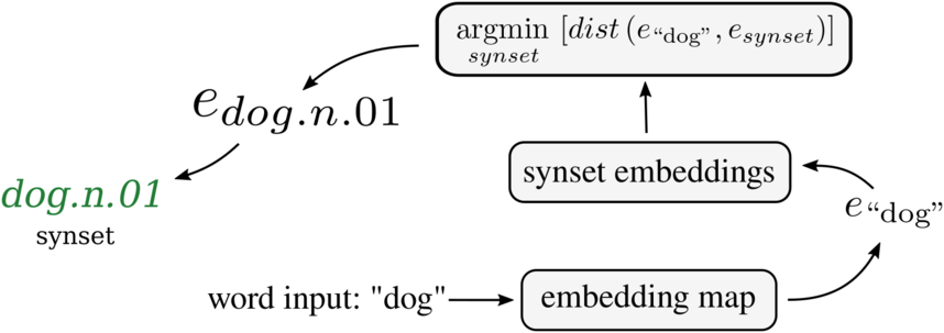

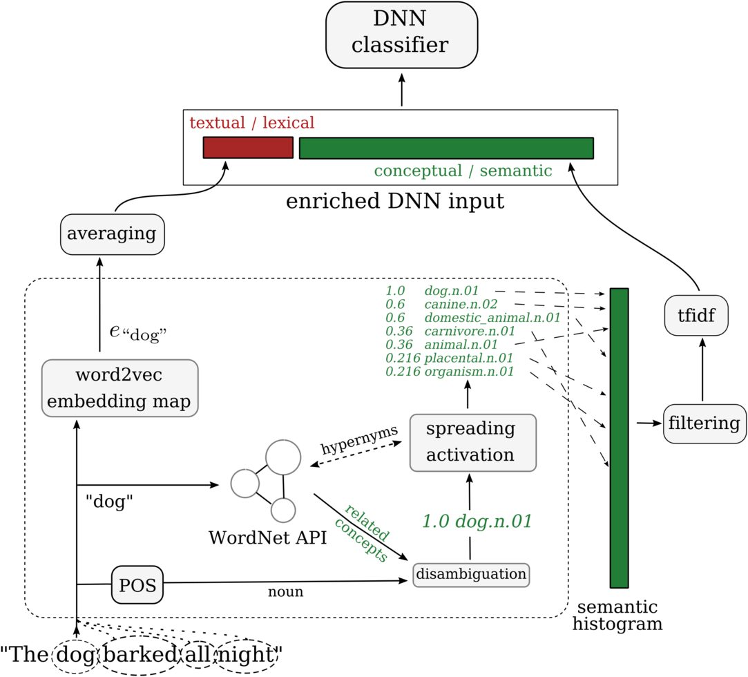


 Open access