


1. INTRODUCTION
Glacier tongues, also known as ice tongues, are the seaward extension of glaciers and can project tens of kilometres into the coastal ocean. They block sea-ice transport and, in conjunction with an offshore wind, support the formation and maintenance of polynyas (Kurtz and Bromwich, Reference Kurtz, Bromwich and Jacobs1985). However, they are typically a few hundred metres thick and so act as a barrier to flow in the upper ocean. Furthermore, at the downstream edge, enhanced mixing in the wake of the glacier tongue can significantly influence local stratification (Stevens and others, Reference Stevens, Stewart, Robinson, Williams and Haskell2011, Reference Stevens2014; McPhee and others, Reference McPhee, Stevens, Smith and Robinson2016). Large, exposed, ice tongues are a particularly Antarctic feature (Greenland's Petermann Glacier Tongue was largely held within its fiord; Johnson and others, Reference Johnson, Münchow, Falkner and Melling2011).
Here we describe some of the first oceanographic data from south of the Drygalski Ice Tongue (DIT; Fig. 1). The DIT is the seaward extension of the David Glacier and is, at the time of writing, the largest of these massive ephemera in existence around the Antarctic coast. The ice tongue itself has been the focus of a number of geophysical studies (Frezzotti and Mabin, Reference Frezzotti and Mabin1994; Van Woert and others, Reference Van Woert2001; Cappelletti and others, Reference Cappelletti, Picco and Peluso2010). One of its primary oceanographic influences is that it forms the southern boundary for the Terra Nova Bay polynya (TNBP), which sits offshore from the Nansen Ice Shelf. The oceanography of the TNBP area is well studied (Budillon and Spezie, Reference Budillon and Spezie2000; Cappelletti and others, Reference Cappelletti, Picco and Peluso2010) with a focus on (i) polynya processes and (ii) the fate of the associated high-salinity shelf water (HSSW), which must ultimately drain away off the continental shelf.

Fig. 1. Location sketch (a) Victoria Land coast and floating glaciers. This is an inset of (b) the western Ross Sea. (c) The DIT locale is fed by the David Glacier (DG) and adjacent to the Nansen Ice Shelf (NIS) and Geikie Inlet (GI). Some operations were based out of Mario Zuchelli Station (MZS) on the shores of Terra Nova Bay which sustains a polynya (TNBP). The sampling in 2012 took place at the SDFC. The image in (c) is courtesy of NASA and is a NASA MODIS 250 m image from mid-October 2012. (d) Elevation slice along DIT (dashed line in panel b) redrawn from Baroni and others (Reference Baroni2002).
The DIT lies over water depths of between 600 and 1200 m, is ~80 km long and 20 km wide, and thins from a grounding line thickness of ~1600 m (Bianchi and others, Reference Bianchi, Chiappini, Tabacco, Passerini, Zirizzotti and Zuccheretti2001) to a thickness of ~170–250 m at its tip (Baroni and others, Reference Baroni2002). However, radar transects suggest that this thinning from the grounding line is not monotonic (Fig. 1d) as the survey work found substantial depth variability at the 2–5 km horizontal scale (Bianchi and others, Reference Bianchi, Chiappini, Tabacco, Passerini, Zirizzotti and Zuccheretti2001; Baroni and others, Reference Baroni2002). The terminus of the DIT has calved substantially as recently as 2006 when iceberg C-16 collided with the tip (MacAyeal and others, Reference MacAyeal2008). Prior to the satellite era, knowledge of glacier scale and its variation was obviously more sporadic. However, in the 100 years prior to the C-16 collision (MacAyeal and others, Reference MacAyeal2008), there is some knowledge around two substantial calving events; one at the start of the 1900s, and a second event ~1955–1957 where the glacier likely halved in length (Frezzotti and Mabin, Reference Frezzotti and Mabin1994). In addition, the Nansen Ice Shelf directly north of the DIT, calved ~200 km2 of ice in April 2016 (Li and others, Reference Li, Ding, Zhao and Cheng2016).
Such a change in the glacier extent affects how the ice tongue interacts with the ocean. Evidence from further south of the DIT suggests that there is a consistent coastal current containing buoyant ice shelf water (ISW) from Haskell Strait (bottom of Fig. 1a), a gateway to the Ross Ice Shelf cavity (RISC) (Robinson and others, Reference Robinson, Williams, Stevens, Langhorne and Haskell2014), northwards along the Victoria Land coast – the so called Victoria Land Coastal Current (VLCC). ISW modifies sea-ice growth and structure (Langhorne and others, Reference Langhorne2015) and so it is important to understand the persistence of ISW waters. If this current persists further north, it will encounter a sequence of floating glaciers flowing off the Victoria Land coast that it must negotiate – with the DIT being the largest (Fig. 1).
Here we consider data from two expeditions; a vessel-based hydrographic survey (late 2014) and a sea-ice camp to the south west of the floating glacier (early 2012). The sea-ice conditions were different in the two visits (with more ice later in the season, Fig. 2). The specific objectives of the present paper are to (i) describe a hydrographic circuit of the glacier, (ii) examine detailed data in the potential ‘stagnation zone’ at the south-west corner of the DIT, (iii) look at the mechanics of the blocking caused by such floating glaciers and (iv) consider the evidence for a coastal current in this region.
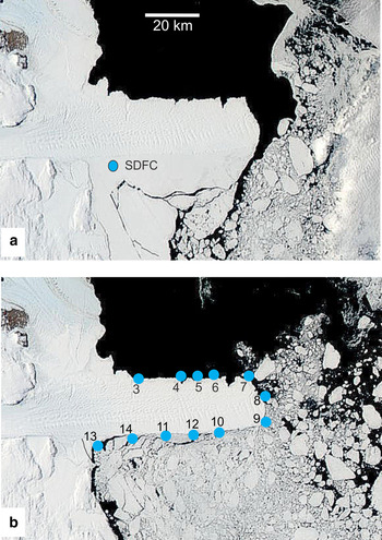
Fig. 2. Sea-ice comparison (a) 30 January 2012 and (b) 26 December 2014. The 2012 image shows the location of the SDFC and the 2014 image shows the location of the CTD profile stations. See (a) for scale bar. Images courtesy NASA MODIS.
2. HYDROGRAPHIC SURVEY IN 2014
Numerous voyages have captured hydrographic data to the north and east of the DIT (e.g., Budillon and Spezie, Reference Budillon and Spezie2000; Cappelletti and others, Reference Cappelletti, Picco and Peluso2010). Knowledge of oceanography to the south has been from much further south, essentially in McMurdo Sound (Lewis and Perkin, Reference Lewis, Perkin and Jacobs1985; Mahoney and others, Reference Mahoney2011; Robinson and others, Reference Robinson, Williams, Stevens, Langhorne and Haskell2014). The data described here are a sequence of conductivity–temperature–depth (CTD) profiles around the edge of the DIT recorded from the IBRV Araon in December 2014 (Fig. 2b) using a Seabird Electronics CTD SBE911plus sampling package. To the best of our knowledge (Bianchi and others, Reference Bianchi, Chiappini, Tabacco, Passerini, Zirizzotti and Zuccheretti2001; Baroni and others, Reference Baroni2002), the DIT is <250 m thick for the majority of the section where profiles were taken.
The data show substantial variations in temperature and salinity (Fig. 3) along the perimeter of the DIT, notably between profiles on the north and south sides. The data show a warm layer, reaching as high as −1°C, in the upper 50 m everywhere except along the eastern tip of the DIT (Stations 08 and 09; Fig. 4). There is evidence of very low-salinity water in the upper ocean to the north of the glacier (), which is most likely meltwater (Souchez and others, Reference Souchez1991). At these temperatures, where the temperature itself has very little influence on density, the temperature structure contains more fine structure than salinity (Fig. 3). There is no obvious signature in the temperature-salinity profiles at the depth of the underside of the DIT (170–250 m) and each side maintains separate temperature–salinity structural character.
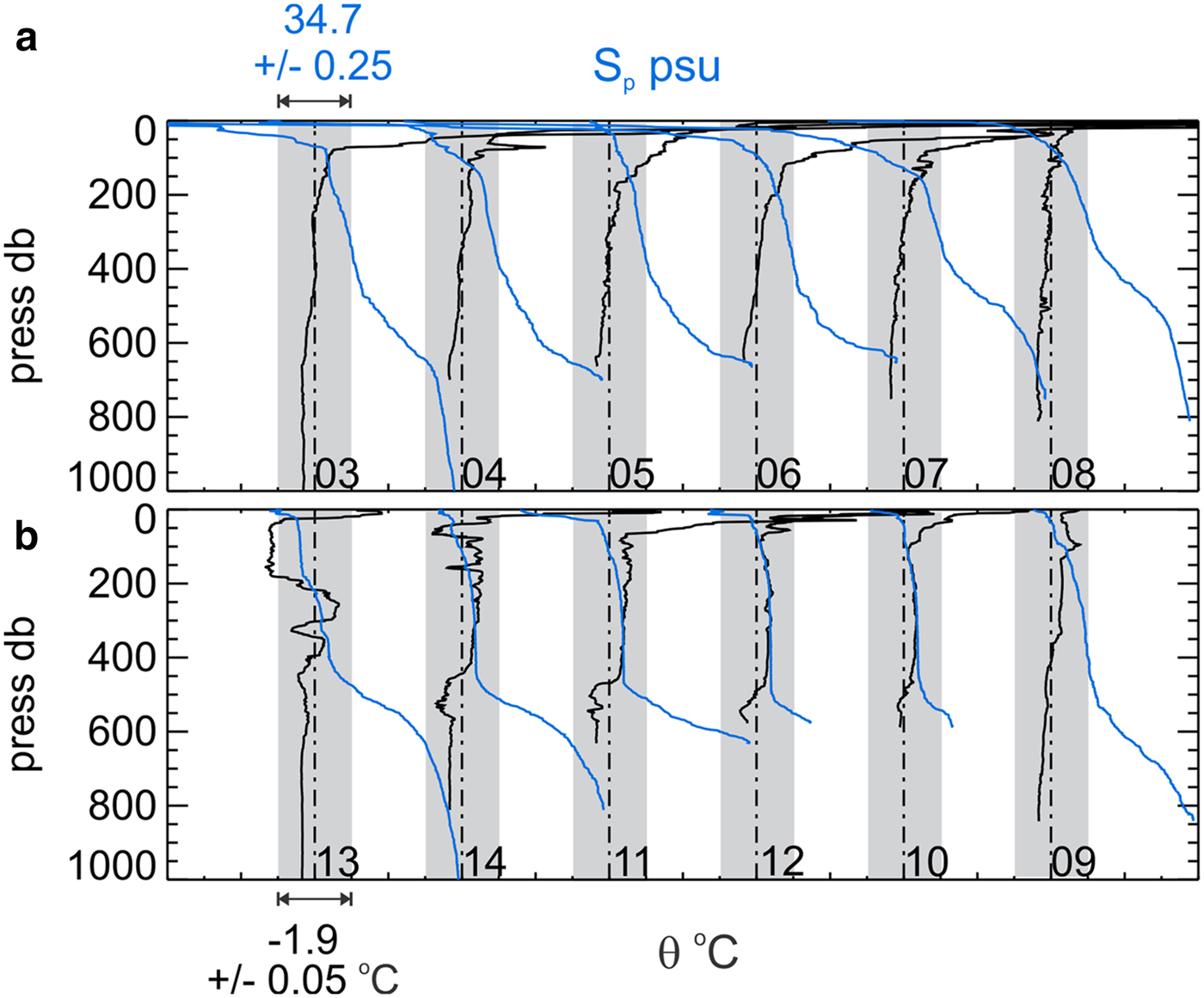
Fig. 3. Potential temperature and practical salinity profiles (offset to the right by 0.1 psu) profiles from stations shown in Figure 2b separated into (a) north and (b) south of the DIT. For temperature the vertical dash-dot line shows −1.9°C and the shaded area spans −1.95 to −1.85°C and for salinity the vertical dash-dot line shows 34.7 psu and the shaded area spans 34.675–34.722 psu.
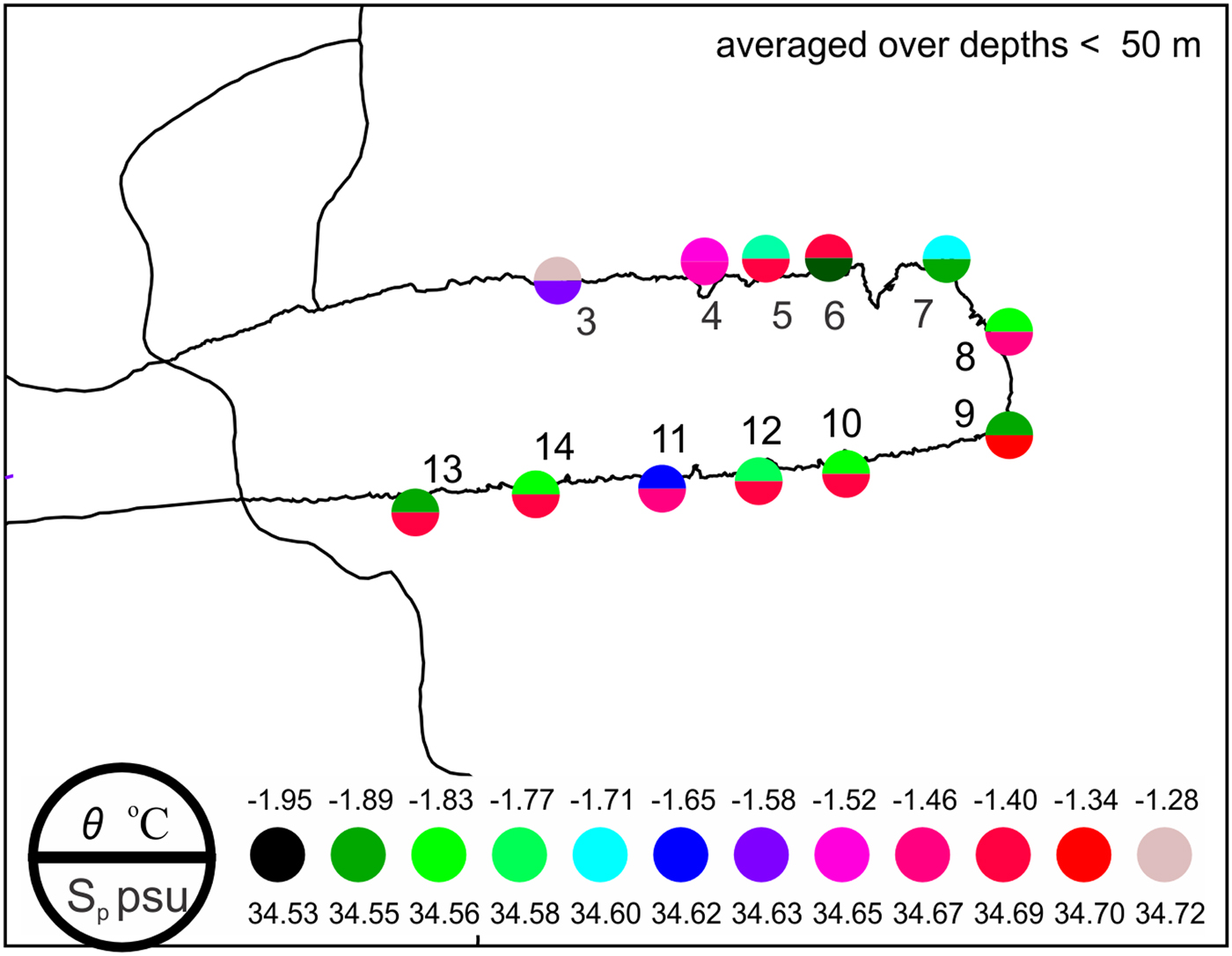
Fig. 4. Averages of potential temperature and practical salinity over the upper 50 m.
The most distinct profile in terms of temperature is at station 13, the closest inshore on the southern side of the DIT (see next section). This is the only station to have (i) in situ supercooled water (30–100 m) and (ii) temperature layering at ~350 m. The profiles at the tip of the DIT have relatively little temperature structure but substantial salinity variation. There are clear haloclines in all profiles over depths ranging from 500 to 600 m.
The near-surface values are difficult to resolve from the profile figures as drawn. The averages of the upper 50 m of each profile (Fig. 4) show the temperatures in the upper 50 m trending from cold in the southwest corner, through mostly warming around to the northwest corner. Near-surface salinity is mostly greater to the south, with a clear shoaling trend moving to the east for the point at which the profile crosses the S p = 34.7 line in practical salinity units. To the north, there is an overall minimum in the northeast, but variability elsewhere.
The temperature data below 600 m collapse on to the same line for north and south of the DIT (Fig. 5), although curiously this does not apply to the more dynamically significant salinity structure. The only indication of a clear signature associated with the base of the DIT (170–250 m) is where the north-side salinity drops away at depths <150 m. The south-side water column is better mixed between 200 and 500 m depth. The salinities in the upper 200 m are lower on the north side, relative to the south side, by ~0.02 practical salinity units (psu).

Fig. 5. The 2014 CTD profiles north (black) and south (pink) of the DIT for (a) potential temperature θ, (b) salinity (psu) and (c) buoyancy frequency squared from westernmost profiles (3 and 13).
Fig. 6. Difference in density from north to south, so a positive value is a larger density to the north (Terra Nova Bay Polynya). Each profile comparison is offset by 0.1 units to the right with the zero marked by a dashed vertical line. Profile numbers correspond to Figure 2b.
The resulting north–south differences in density (Fig. 6) are significant, reaching 0.03 kg m−3 at depth, and much larger in the upper 100 m. For depths >100 m, the northern side is typically denser, with the reverse being true in the upper 100 m. This reversal in density difference is the clearest evidence of the presence of the base of the glacier in the CTD data. The potential temperature–salinity distribution (Fig. 7) shows that all water with salinity above 34.75 psu (i.e. mainly deep) is likely ice shelf influenced, and in some of the south-side data, there is also evidence of shelf basal melting because temperatures are below the surface freezing temperature. Budillon and Spezie (Reference Budillon and Spezie2000) described the water masses on the north side of the DIT. They identified summer surface water (−1.7 < θ<1.5°C, 33 < S p < 34.5 psu), Terra Nova Bay ice shelf water (TNBISW; θ < −1.92°C, 34.72 < S p < 34.82 psu) and HSSW (θ~−1.91°C, 34.75 < S p psu). In terms of these definitions, no summer meltwater was seen to the south of the DIT in the present 2014 data, although the water was sufficiently warm near the surface. The only TNBISW seen was on the south side and at the lower end of the salinity range. The HSSW is very clear beneath ~550 m. We observe for the first time cold and relatively fresh water (θ < −1.9°C, 34.68 < S p < 34.74 psu) high in the water column on the southern side of the glacier. This is most apparent in the westernmost station from 2014 (13), which is close to the location of the 2012 South Drygalski Field Camp (SDFC).

Fig. 7. Key focal region of potential temperature vs salinity diagram for the 2014 hydrographic survey CTD data. The dashed line is the freezing temperature and the blue region (R14) are observations further south towards Haskell Strait described in Robinson and others (Reference Robinson, Williams, Stevens, Langhorne and Haskell2014). The inset shows the full dataset. Regions of HSSW, TNBISW and summer surface water (SSW) from Budillon and Spezie (Reference Budillon and Spezie2000) are shown.
3. SDFC, 2012
A 9-d field camp on the fast ice (SDFC, Fig. 2a) was located in the vicinity of the area of interest identified by the hydrographic survey. The MODIS imagery spanning the period of interest in this paper (Fig. 2) illustrates how variable sea ice in the region can be during the December–January period. Coherent fast ice around the start of the year extended well south at the longitude of the tip and was apparent around the time of our sampling. Within 4 d after our departure from the 2012 fast ice camp, the ice in the region started breaking up. Katabatic winds are less common at this time of year (Rusciano and others, Reference Rusciano, Budillon, Fusco and Spezie2013), despite this the entire region to the north of the DIT remained ice free, suggesting recent katabatics, combined with solar warming, was sufficient to keep the area open.
The field camp was 2 km to the south of the DIT (75o 31.655′S, 163o 30.924′E) off shore from Geikie Inlet (Fig. 1c), accessed using helicopters flying from Mario Zuchelli Station (Italy) – a distance of 90 km. The fast ice in the region at the time was 1.9 m thick. Jeffries and Weeks (Reference Jeffries and Weeks1992) accessed the region (although more to the east) from helicopter to collect sea ice cores and found evidence of deep basal ice melt (i.e. platelet ice crystals). In the 2012 work here, a video camera was lowered down the profiling hydro-hole to look back up at the sea ice underside. Frame-grabs from this provided images that revealed the presence of platelet crystals (Fig. 8a). This imagery also showed that the ice underside, while not heavily ridged, was lumpy and rough – certainly not smooth as would be expected in a melting situation – i.e., implying growth or crystal attachment.

Fig. 8. Frame-grabs from under-ice video camera from SDFC. (a) Image shows ice platelet structure in the sea ice (based on other images in the sequence with the ADCP frame in view, the field of view here is ~50 cm). (b) Wide angle view (at an angle) showing billowy nature of underside of the sea ice.
Currents in the upper 50–80 m of the water column were recorded using a Teledyne-RDI 300 kHz ADCP mounted just beneath the underside of the sea ice and pointing downwards. The data cover 17–26 January 2012 with the uppermost depth (relative to water surface) bin at 4.20 m (ice thickness 1.9 m) and the bins were 2 m in size. The instrument collected 120 pings per ensemble, which were at 2 min intervals and a magnetic declination offset of 133° was applied. Our sampling was from around spring tides of the typically 1 m peak–peak tidal elevation range (Fig. 9a, see tbone.biol.sc.edu). The velocity data contained a reasonable tidal signature, mainly seen in the v (north–south axis) component although notably the peak speeds appear after the maximum in the spring tide. The non-tidal variability is mainly seen in the u (east–west) component (Fig. 9b). After around the midpoint of the dataset (22 January 2012), the east–west flow increased substantially to an amplitude of ~0.15 m s−1 (Fig. 9c). These flows are substantially slower than the 1 m s−1 inferred by Legresy and others (Reference Legresy, Wendt, Tabacco, Remy and Dietrich2004) in order to explain the flexure observed in the Mertz Glacier Tongue. The backscatter amplitude (Fig. 9d) is comparable with that seen elsewhere in the region – a general reduction in return signals at ~80 m limiting deeper velocity estimation. The faster variability in acoustic backscatter at a depth of ~48 m exhibited vertical displacements of 20 m and is likely a combination of a number of factors including the presence of phytoplankton, light and ice crystals. The backscatter also exhibited a couple of quite large periods of backscatter reduction (although there was still sufficient return information to resolve velocity) at times (end of day 21 and start of day 25). The day 21 change coincides with the start of the faster flow to the east and possibly relates to some change in reflectance associated with a water mass frontal region.

Fig. 9. (a) Tidal amplitude from TideX (shaded boxes are VMP sampling) and ADCP data from the 2012 field camp at SDFC showing (b) eastward (positive u), (c) northward (positive v) and (d) backscatter amplitude. The white regions in (b) and (c) represent areas of insufficient signal resolve a reliable velocities.
A Rockland VMP500 (Victoria, Canada) microstructure loose-tethered free-fall profiler quantified both CTD and turbulent dissipation rate data (Wolk and others, Reference Wolk, Yamazaki, Seuront and Lueck2002). Operational constraints meant only 18 profiles were possible. Profiles of temperature and salinity over the upper 200 m were recorded using a Seabird Electronics (SBE, USA) temperature (SBE 3) and conductivity (SBE 4) sensor pair mounted on the VMP500. These sensors were factory calibrated, 6 months prior to experiment. The sensors were un-pumped so as to not affect the shear data through the creation of vibration. This meant that the spatial resolution of the salinity was several metres. However, salinity spiking was not particularly apparent due to the very low dynamic range in temperature. When in use, the profiler was kept in the water continuously during the experiment so that the packages were equilibrated to the ambient temperature, reducing thermal inertia effects.
These late January CTD data from the VMP500 (example shown in Fig. 11a) consistently showed a warm shallow layer at ~20 m capped by a fresher layer, suggesting the sea ice was melting from beneath. Deeper in the water column, the temperature decreased to below the surface freezing temperature at a depth of ~100 m. In the example shown in Fig. 10, this coincided with a temperature inversion with an overturning length-scale of ~20 m, although the salinity compensation means this does not generate a density inversion. Beneath this, the water column had pronounced interleaving layers in temperature. The entire 2012 profile is fresher than seen in the 2014 data, which also had different sea-ice coverage (Fig. 2). The 2012 CTD data, limited though they are, clearly show water beneath the local freezing point, which is taken generally as evidence of ISW (Leonard and others, Reference Leonard2006). A curious aspect of the profiles is that there was often interleaving at the depth where the potential temperature drops beneath the surface freezing temperature, i.e., the top of the ISW layer (dashed box in Fig. 10a). Stevens and others (Reference Stevens, Robinson, Williams and Haskell2009) considered diffusive arguments to suggest that RISC water could make it as far north as the DIT. However, applying that analysis this far from the RISC implies the water would only be weakly supercooled and interfaces likely indistinct. Instead, the scalar profiles show a clear delineation at the point of moving to supercooled conditions and the structure is layered in nature. This suggests that the ‘ISW’ was produced close by and recently.
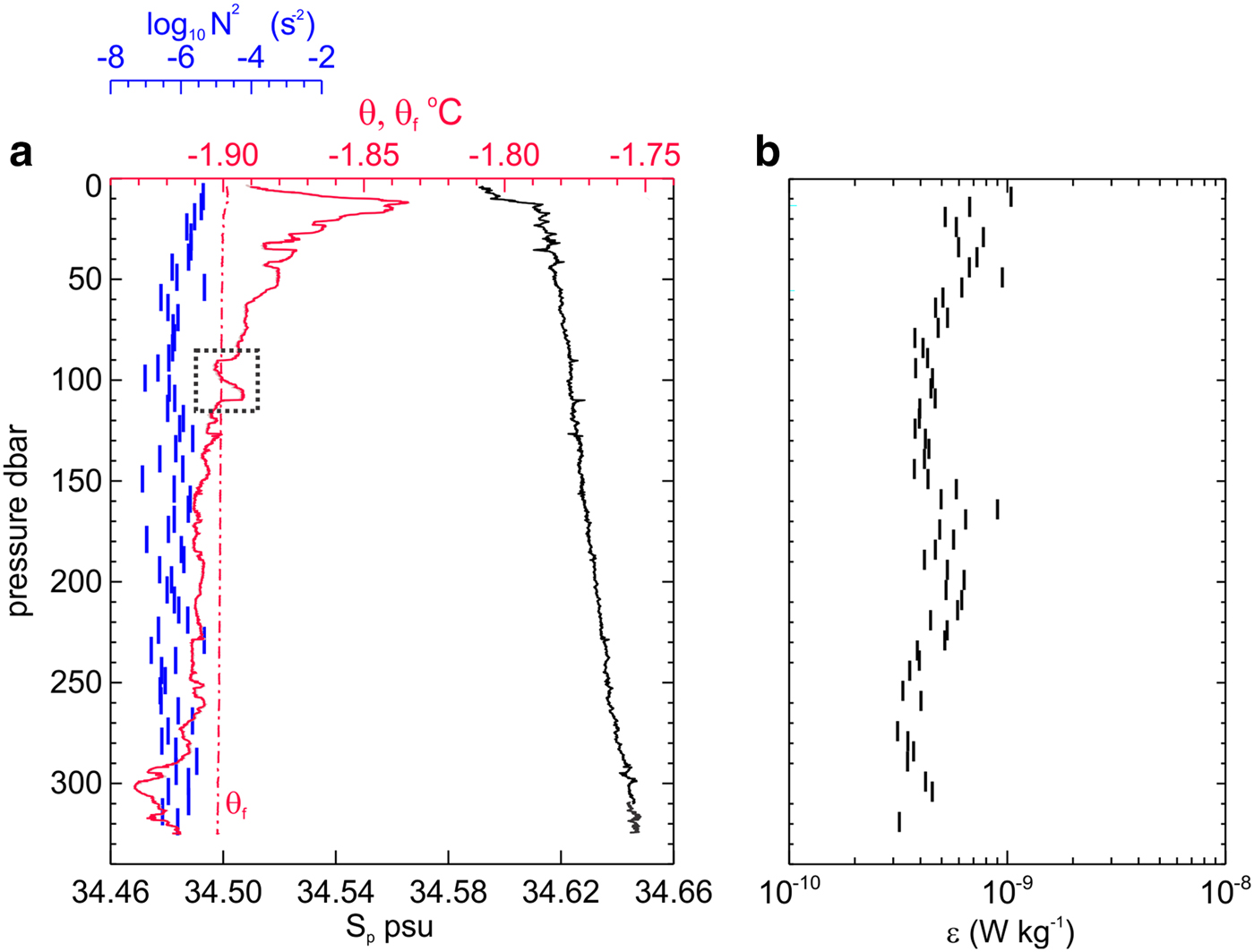
Fig. 10. CTD and microstructure profile data from SDFC on 21 January 2012 (middle of that day, local time) showing (a) potential temperature, salinity and buoyancy frequency squared. The dash-dot line is the surface freezing temperature. (b) Dissipation rate. The spikiness in the salinity profile is an artefact of not pumping the sensor and the dashed box is discussed in the text.

Fig. 11. Energy dissipation rate distribution from SDFC, for all 18 VMP250 microstructure profiles where vertical axis is number of 10 m sample bins.
The shear profiler enabled estimation of the turbulent energy dissipation rate ε (m2 s−3 = W kg−1) and the method has been used in such conditions previously (Robertson and others, Reference Robertson, Padman and Levine1995; Stevens and others, Reference Stevens, Stewart, Robinson, Williams and Haskell2011; Fer and others, Reference Fer, Makinson and Nicholls2012). Energy dissipation rates were resolved from the dual shear probe profiler using standard techniques (Wolk and others, Reference Wolk, Yamazaki, Seuront and Lueck2002; Stevens and others, Reference Stevens, Stewart, Robinson, Williams and Haskell2011). The turbulence measurements (Fig. 10) were highly constrained by operations and were mostly during lower flow periods (Fig. 9a). However, this proves useful for defining lower bounds for mixing in what is potentially a stagnation point whereby northward flow might be trapped against the southwestern corner of the glacier. The data show the dissipation rate barely exceeding the noise flow (~10−10 W kg−1) with a mean at 6 × 10⁻¹⁰ W kg−1 (Figs 11a and 12). This is indicative of very low levels of turbulent mixing. The buoyancy frequencies N are not particularly low, possibly due to the presence of meltwater, so the vertical diffusivities (~0.2ε/N 2) are low (~10−5 m2 s−1) but greater than molecular rates (~10−7 m2 s−1 for heat).

Fig. 12. Schematic of surface flow past ice tongue showing scales associated with (a) plan and (b) elevation views and (c) NASA MODIS image from 11 February 2016, showing sea ice swirl off tip of the DIT.
4. DISCUSSION
Clearly, floating glaciers act as a blocking feature to the upper ocean whereby the buoyancy-driven surface current is either forced around or underneath the floating barrier (Fig. 12). This is analogous to gravity current flow around and over a ridge under the influence of rotation (Wang and others, Reference Wang, Danilov and Schröter2009). The driving pressure gradient must be balanced by the forces associated with rotation and the changes in flow associated with the geometric dimensions of the obstacle. Consequently, we expect the forces driving ocean variability to be dependent on the size of the obstacle (Deleersnijder and others, Reference Deleersnijder, Norro and Wolanski1992). A fundamental difference between the DIT and the much smaller Erebus Glacier Tongue (e.g. Stevens and others, Reference Stevens2014) to the south, is the width. The ratio of tidal excursion to glacier width for the DIT is substantially <1, whereas it is >1 for the Erebus Glacier Tongue (Stevens and others, Reference Stevens2014). This means that, in the case of the DIT, the transit time beneath the glacier relates to the buoyancy-induced pressure gradient, which is in-part a function of the regional circulation. However, tides may still play a role in terms of pumping and local supercooling.
In order to identify the key processes controlling flow around the glacier it is useful to consider the mechanistic scaling for a temporally steady-state momentum balance for the buoyant flow moving north along the coast. We expect the advective acceleration terms to balance the rotation, pressure (baroclinic) and friction components (as described in Table 1). Following the approach of Vennell (Reference Vennell1998) we can replace these terms with scaling equivalents for an order of magnitude look at the controlling processes. Vennell (Reference Vennell1998) specified a priori that the imposed pressure gradient must be balanced by the remaining terms: here the northward steady flow is the driver. Assuming the background northward flow u 0 is affected by the DIT (width W, length L, thickness h g) in water depth H then there will be friction (τ) and baroclinic pressure gradient components (∂ζ/∂y). Scaling representations are laid out in Table 1 along with estimated quantities. The advective term sees the velocity change over the length of the glacier. The across-stream velocity used in the rotational component is harder to define mechanistically so here it is the along-stream speed scaled by the aspect ratio of the glacier. The baroclinic pressure gradient uses the top to bottom density difference. There are three scenarios that can be envisaged. The first is the transient whereby a northward flowing surface flow commences and, as it piles up against the south edge of the DIT, the pressure gradient is opposed to the flow. The second scenario is where a steady state equilibrium whereby the northward flowing water has filled up the surface waters to the south of the DIT to the depth of the underside of the ice tongue and so, as it spills under the glacier, the pressure gradient drives a northward flow. Both scenarios relate to vertical displacement of the mean density profile. The third scenario is a modification of the first, but now influenced by processes to the north of the DIT. Density profiles to the north are in fact heavier, at least below 150 m (Fig. 5), so empirically there is a baroclinic pressure gradient opposing the flow. The final scaling component, friction, is distributed over the water column beneath the glacier (H-h g). Alternatively, stratification might confine this scale to an extent.
Table 1. Northward (+y) momentum equation, scaling equivalent and magnitude
Here we use the following representative values: u 0 = 0.05 m s−1, L = 80 km, f = 1.4 rad s−1, W = 15 km, h g = 200 m and c d = 0.001. The g′ is based on N 2 = 10−6 (rad s−1)2 for the initial consideration based on (a) vertical displacement and (b), an opposing Δρ = 0.03 kg m−3 (see text).
Table 1 indicates that the baroclinic gradient is essentially balanced by the rotational forcing. This supports the notion that the leakage through the tongue-underside channels, which will affect this baroclinic pressure gradient, is important, as is the observed opposing density gradient. Clearly, in sea-ice patterns at least, there are examples showing an eastward surface flow (Fig. 12c) on the southern side of the DIT. This suggests the northward flow south of the glacier is constrained by rotation, so turning eastward and flow along the glacier until reaching the terminus, while also losing some volume beneath the glacier, possibly through channels (Fig. 1d). It will only be weakly opposed by the background pressure gradient as Figure 6 indicates the north–south density differences are smaller than the vertically displaced profile would generate.
With along-glacier variations in DIT thickness of as much as a hundred metres (Bianchi and others, Reference Bianchi, Chiappini, Tabacco, Passerini, Zirizzotti and Zuccheretti2001; Baroni and others, Reference Baroni2002) there will clearly be favourable pathways for buoyancy-driven flow (Fig. 1d). This might be a reason why the thickness of the glacier is not obvious in the CTD profiles as cross-glacier flow will occur at a range of depths. Bianchi and others (Reference Bianchi, Chiappini, Tabacco, Passerini, Zirizzotti and Zuccheretti2001) separated nine floating glaciers into three classes – all of the Victoria Land glaciers fall into the ‘rippled’ category and they suggest that the different classes potentially relate to factors like ‘sea circulation’ so that there might be a feedback effect from the coastal flow. This suggests the view shown in Figure 12 whereby the underside is not flat but a channelled zone, which will result in a highly three-dimensional leeward side to the ocean flow. Thus, one expects spatially separate plumes to enter the polynya region, assuming a northward flow, which potentially explains the variability in salinity seen in Figure 4 to the north of the DIT (whereas temperature might be controlled by the proximity to the glacier). This provides strong motivation for new oceanographic horizontal survey tools such as ocean gliders and autonomous underwater vehicles.
The scalar salinity and temperature properties along the sides of the DIT can be compared (Fig. 7) with those seen further south in McMurdo Sound (Robinson and others, Reference Robinson, Williams, Stevens, Langhorne and Haskell2014) and in TNBP itself (Budillon and Spezie, Reference Budillon and Spezie2000). The DIT data are less saline than the observations described in, and around, Terra Nova Bay in the late 1990s (Budillon and Spezie, Reference Budillon and Spezie2000). However, the DIT data, while warmer, are in the right salinity range to have evolved from the conditions further south (Robinson and others, Reference Robinson, Williams, Stevens, Langhorne and Haskell2014) providing some evidence of the persistence of a coherent VLCC moving northwards. That such a current exists is almost certain from the perspective of the basin scale gyre (Dinniman and others, Reference Dinniman, Klinck and Smith2003; Jendersie, Reference Jendersie2016) and the scalar transect data of Robinson and others (Reference Robinson, Williams, Stevens, Langhorne and Haskell2014).
The mechanics at play here are unique to Antarctica, requiring ice shelf meltwater and large floating glaciers. Despite this, the topic is of global relevance due to the influence of such floating structures on polynya processes. This in turn feeds through to both HSSW and sea-ice production. This study suggests the pre-conditioning of the sea water prior to arrival in the polynya region is a complex balance of processes. The ocean current is relatively buoyant due to the influence of basal meltwater. The resulting pressure gradient then drives flows that are acted upon by rotation and constrained by the coast and the glacier itself. If the flow gains enough heat in the intervening time it will serve to generate more basal melting that, in turn, maintains the buoyancy that drives the flow.
The work generates new questions regarding the regional behaviour both in terms of the VLCC and if the DIT were to substantially calve. Also it suggests that there may be significant influences due to the smaller, but still substantial, glacier tongues in the region. It may be that the flow beneath the smaller ice shelves on the Victoria Land coast (e.g. Tison and others, Reference Tison, Ronveaux and Lorrain1993) also plays a role in pre-conditioning the TNBP as well as the smaller polynya in the region. This work contributes to the understanding of the fate of coastally bound VLCC outflow from the RISC and ice shelf/ocean interactions in general. The VLCC transports ISW northward from the RISC and also serves to connect the relatively small, oceanographically unsampled, but nearby ice shelves along this coastline. The coastal transport embodied in the VLCC controls the degree to which these smaller cavities affect polynya and sea-ice formation.
ACKNOWLEDGEMENTS
We thank the Korea Polar Research Institute (PM16020), the Italian Programma Nazionale di Ricerche in Antartide, the Royal Society of NZ Marsden Fund, the Deep South National Science Challenge, the New Zealand Antarctic Research Institute and Antarctica New Zealand for support. Carlo Baroni provided access to mapping for the area and valuable discussions and Choon-Ki Lee (KOPRI) provided outline data of the glacier. David Gwyther and Tim Stanton are thanked for their comments on an early manuscript, as is the Scientific Editor Laurie Padman. We also thank Helicopters New Zealand Team (Bob, Giles and Wayne), Tim Haskell, Chris Zappa, the staff at Mario Zuchelli and Jang Bogo Stations and Scott Base, and the crew of the IBRV Araon. We acknowledge the use of Rapid Response imagery from the Land, Atmosphere Near real-time Capability for EOS (LANCE) system operated by the NASA/GSFC/Earth Science Data and Information System (ESDIS) with funding provided by NASA/HQ.


 Open access