


1. INTRODUCTION
Global Positioning System (GPS) is the most widely used positioning and navigation technology. Differential GPS (DGPS) offers centimetre-level positioning accuracy for static observations and sub-decimetre accuracy for kinematic systems. However, GPS is a line-of-sight system and is, therefore, unusable or severely limited by signal availability in GPS-challenged environments. GPS is also subject to intentional (jamming) and unintentional RF interference. To overcome these limitations, many navigation technologies based mainly on the concept of multi-sensor integration have been proposed and tested (Mirabadi et al., Reference Mirabadi, Schmid and Mort2003; Sharaf and Noureldin, Reference Sharaf and Noureldin2007; Grejner-Brzezinska et al., Reference Grejner-Brzezinska, Toth, Sun, Wang and Rizos2008; Lee and Jekeli, Reference Lee and Jekeli2011).
In the concept of Collaborative Navigation (CN), each vehicle (also referred to as node hereafter) in the network share information (e.g. GPS code pseudo-ranges, carrier-phase pseudo-ranges or its 3-Dimensional (3D) coordinates, and the inter-nodal distance measurements with other nodes) to improve the overall performance of a group of vehicles. It is assumed that each node of the network can measure the 3D relative position by various inter-nodal ranging techniques such as laser ranging, microwave ranging and vision sensors. The CN can improve the accuracy of a single-platform navigation solution, increase the integrity of its solution, and detect possible collision causes of the vehicle. Figure 1 illustrates the network-based collaborative navigation concept where sub-networks of nodes navigating jointly could be created ad hoc, as indicated by the circles; it should be noted that some nodes (users) may be parts of different sub-networks. In a whole network, the selection of a sub-network of nodes is a critical issue, as in the case of a large number of users in the entire network, computational and communication loads may not allow for the entire network to be treated as one entity (Grejner-Brzezinska et al., Reference Grejner-Brzezinska, Toth, Li, Park, Wang, Sun, Gupta, Huggins and Zheng2009). Conceptually, the sub-networks can consist of nodes of equal hierarchy or may contain a master (anchor) node that will normally have a better set of sensors and will be collecting measurements from all other nodes to perform collaborative navigation.
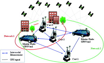
Figure 1. Collaborative navigation concept.
Various collaborative navigation technologies based on the multi-sensor concept have been discussed in many literatures. (Sanderson, Reference Sanderson1997) employed the range measurement in the centralized linear Kalman filter framework. (Fox et al., Reference Fox, Burgard, Kruppa and Thrun1999) proposed collaborative mobile robot localization based on a probabilistic navigation algorithm. (Berefelt et al., Reference Berefelt, Boberg, Nygårds, Strömbäck and Wirkander2004) showed that the relative vector method was better than the other two methods (virtual satellite and shared pseudorange) to improve the GPS/INS performance in urban navigation. (Panzieri et al., Reference Panzieri, Pascucci and Setola2005) used a bank of interlaced Kalman filters to incorporate ranges into the states of the filter. (Brown and Nordlie, Reference Brown and Nordlie2006) designated the master nodes to improve the navigation performance of the entire network. (Kaba and Wu, Reference Kaba and Wu2009) developed the distributed multi-sensor fusion to bind the position errors using GPS, RF beacons, or anchor nodes for the collaborative navigation system. (Grejner-Brzezinska et al., Reference Grejner-Brzezinska, Toth, Li, Park, Wang, Sun, Gupta, Huggins and Zheng2009) employed the bank of extended Kalman filters to integrate the inter-nodal range measurements with other sensor.
Collaborative navigation has advantage over the single vehicle navigation because the position errors of some nodes can be compensated by known (or more accurate) coordinates of other nodes, which improves the overall navigation results of the group of users navigating together. It should be noted that previous studies of the network-based approach use primarily the distance-dependent weighting or the empirical covariance, thus, the accuracy and reliability of a single user or a group of users may not be significantly improved. In this paper, three statistical network-based collaborative navigation algorithms, namely the Stochastic Constrained Least-Squares Solution (SCLESS), the Best Linear Minimum Partial Bias Estimation (BLIMPBE), and the Restricted Least-Squares Solution (RLESS) are proposed and compared to the Kalman filter, based on the field data collected by a network of five kinematic platforms; a GPS Van, a mobile cart and three GPS stations.
2. NETWORK-BASED COLLABORATIVE NAVIGATION ALGORITHM
The relative component of the inter-nodal vector between nodes i and j is given as:
where:
d ij is a single component of the actual distance measurements between two nodes.
x i and x j are the position coordinates of each node.
The inter-nodal output measurement (i.e., sensor output) is simply modeled as equation (2) with additive noise v:
where v is assumed to have Gaussian distribution (v∼N(0,R v), where R v is the noise covariance matrix.
The three-dimensional measurement model for the n-node network environment is given as:
where:
 is the vector of x, y, z difference of inter-nodal distance measurements.
m is the number of measurements.
- is the vector of position in x, y, z for all nodes in the network.
A is the design matrix that linearly relates the node variables through the inter-nodal measurements, and
is the additive noise vector.
Since the design matrix A shows the relationship of the relative inter-nodal measurements for pairs of nodes, it can be written as a composite matrix of identity matrices. The dimension of matrix A is 3 m by 3n for the three dimensional coordinates. In the examples shown here, it is assumed that there is only one user node and other nodes are all reference (or higher order) nodes in a network. Thus, for instance, if the number of nodes is three, there are two inter-nodal distance measurements between the user node and two reference nodes d 31 and d 32 in Figure 2b, then the matrix A is given as follows:
where each I is a 3 by 3 identity matrix for the 3D case.
Figure 2. The geometry of networks studied here as a function of a number of nodes: ▲: reference node, ![]() : user node.
: user node.
However, there is one more inter-nodal relationship between node 1 and 2, d 21, dashed line, see Figure 2b; and thus, one more inter-nodal relationship can be added to the measurements. Therefore, the matrix A can be rewritten as follows:
Similarly, if the number of nodes is 4 (5), one can consider 3 (6) inter-nodal distances among the reference nodes and 3 (4) inter-nodal distances between the user nodes and the reference nodes. Naturally, with the increasing number of nodes in the network, more inter-nodal measurements can be obtained and measured. Therefore, the proposed ‘Network-based Estimation’ method can provide stronger geometry, as compared to a single distance measurement, as well as the redundancy.
Three network-based collaborative navigation algorithms, namely:
(1) RLESS which employs the minimum constraints to overcome the rank deficiency by fixing one of the known positions;
(2) SCLESS which imposes the stochastic constraints on the unknown position using a priori coordinate variance and
(3) BLIMPBE which minimizes the biases for a subset of parameters (the position) are tested in a network composed of the various kinematic nodes with the objective to compare, evaluate, and, ultimately, to identify the best method for collaborative navigation.
The general measurement (observation) model is shown in Equation (3) and is recalled as:
where:
- is the 3m×1 inter-nodal measurement vector of x, y, z components.
A is the 3m× 3n design matrix with rank of q (q⩽n), x is 3n×1 unknown vector of position difference in x, y, z.
- is the additive noise vector assuming the normal distribution with zero mean and variance-covariance of Σ.
σ 02 is the unit-less variance component.
P is the weight matrix of the measurements.
2.1 Restricted Least-Squares Solution (RLESS)
In the RLESS, the minimum constraint is given by fixing the best known coordinates in a network. For example, if there are two reference nodes and one user node, one reference node which has the best accuracy (e.g., master node) is fixed for a minimally constrained adjustment. Thus, it could be the best approach if only one node has high accuracy coordinates.
The minimally constrained solutions are obtained using the following constraint equation:
where:
κ 0 is the l×1 constraint vector.
K is the l×m corresponding coefficient matrix and rank(K)=n−q.
q is the number of coordinates fixed.
The following estimate and the corresponding variance-covariance matrix for the unknown vector, ![]() , can be obtained using the general least-squares method:
, can be obtained using the general least-squares method:
where [N c]=AT P [A y].
Alternatively, the estimate and corresponding covariance matrix for the RLESS can be obtained using the general recursive least-squares method (see the detailed derivations in Lewis, Reference Lewis1986).
2.2 Stochastically Constrained Least-Squares Solution (SCLESS)
If prior information about the nodes is available (e.g., known or best approximation of the coordinates of the nodes) with their variance-covariance matrix, the SCLESS method can be used. Similar to Equation (7), the constraints with random errors are formulated as:
where:
z 0 is the l×1 stochastic constraints vector.
e 0 is the corresponding random errors with zero mean and variance-covariance of Σ 0.
P 0 is the positive-definite weight matrix.
The rank of K matrix is l⩾m−q.
Since the observation vector and the stochastic constraints are uncorrelated, the least-squares estimates, ![]() , and the variance-covariance matrix,
, and the variance-covariance matrix, ![]() , of the unknown vectors are:
, of the unknown vectors are:
2.3 Best Linear Minimum Partial Bias Estimation (BLIMPBE)
Finally, the BLIMPBE, which was originally developed to minimize the biases at a specific receiver positions in a rank-deficient GPS network adjustment, estimates the unknowns with the minimum biases using the selection matrix (Schaffrin and Iz, Reference Schaffrin and Iz2001; Snow, Reference Snow2002). For example, if two reference nodes have better accuracy than all other reference nodes (i.e., the number of all nodes is more than three) one can employ only two reference nodes in the BLIMPBE method using a selection matrix. The SCLESS uses all reference nodes in a network, while the BLIMPBE employs only selected reference nodes. Therefore, it could be the best approach if one can find (or select) the best reference nodes among all reference nodes in the network.
The selection matrix, which has the following form, should have sufficient rank to overcome the rank-deficiency in the system.
where I 3×3,s is the 3 by 3 identity matrix with the dimension of s according to the number of selected reference nodes from the entire network.
Since the detailed derivations are available in ibid., the resulting estimates, ![]() , and the corresponding variance-covariance matrix,
, and the corresponding variance-covariance matrix, ![]() , are given at Equations (14) and (15):
, are given at Equations (14) and (15):
3. CENTRALIZED KALMAN FILTER
The Centralized Filter (CF) represents globally optimal estimation accuracy for the implemented system models (Knight et al, Reference Knight, Osborne, Snow and Kim1993; Grejner-Brzezinska and Wang, Reference Grejner-Brzezinska and Wang1998; Carlson, Reference Carlson2002; Zhang et al., Reference Zhang, Lennox, Goulding and Wang2002). A CF may lead to significant computation loads, but it serves as an ideal benchmark for other filters. Therefore, in this paper, we implemented a centralized linear Kalman filter and compared its performance with respect to three proposed network-based collaborative navigation algorithms. In Figure 3, all measurements collected at the nodes and the inter-nodal range measurements are processed by a single centralized Kalman filter. Figure 3 illustrates a generic case, when non-linear measurements and/or dynamic model are used, while in the examples presented here a linear Kalman filter is used.
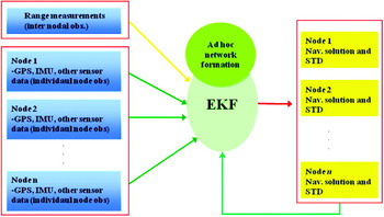
Figure 3. Centralized filter for collaborative navigation.
The full derivation of the linear Kalman filter for collaborative navigation is well presented in (Sanderson, Reference Sanderson1997). Here, only a summary is given.
A linear measurement model of collaborative navigation can be described as the random variable, ![]() , which is the vector of nodes position with a priori distribution, P k−1, and measurements is given as
, which is the vector of nodes position with a priori distribution, P k−1, and measurements is given as ![]() , with covariance matrix, R v. Based on Gaussian probability density function the linear measurement model can be solved as the minimum mean-square error estimation of the Kalman filter.
, with covariance matrix, R v. Based on Gaussian probability density function the linear measurement model can be solved as the minimum mean-square error estimation of the Kalman filter.
A linear estimator, ![]() , for nodes positions,
, for nodes positions, ![]() , is given as
, is given as
where:
matrix H k shows the relationship between states and inter-nodal range measurements.
R v is the covariance matrix of the inter-nodal range measurement errors.
The covariance of the estimates is given as:
4. FIELD TEST AND SIMULATION
To evaluate the network-based collaborative navigation algorithms, a field test was performed on 11 August. 2009 on West Campus at The Ohio State University. The three GPS stations and two mobile platforms (referred to as ‘GPSVan’ and ‘mobile cart’), were used in the test. In the GPSVan, there are two navigation-grade IMUs and two geodetic-grade GPS receivers, while the mobile cart carries a tactical-grade IMU, two GPS receivers and a 12 volt battery (Figure 4). The GPSVan and the cart were moved along the varying-dynamic trajectories around the three GPS base stations (Figure 5).
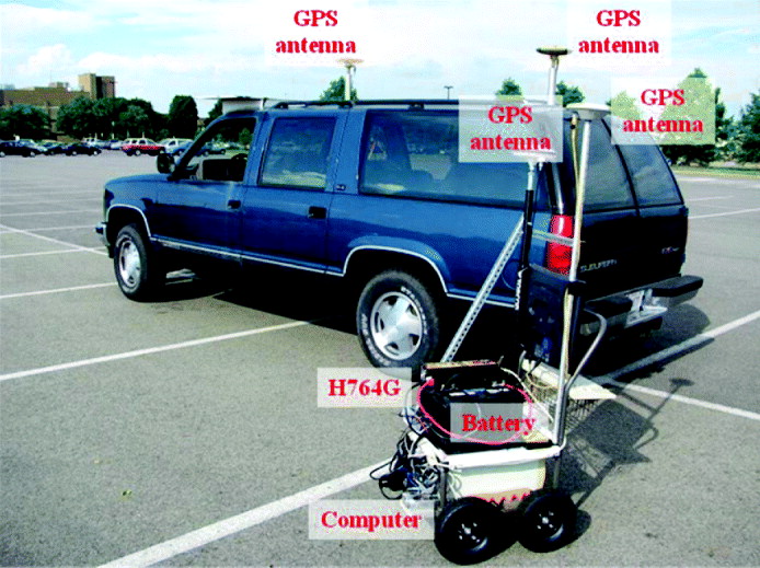
Figure 4. ‘GPSVan’ and ‘mobile cart’.
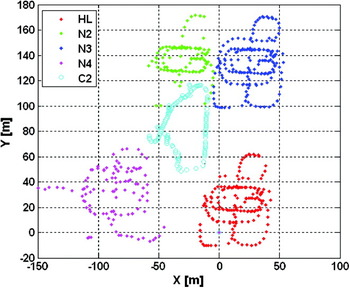
Figure 5. The simulated trajectory of the five nodes.
To process the kinematic GPS data, the AIMS-Pro software ver. 2.0, developed at the Satellite Positioning and Inertial Navigation (SPIN) Laboratory at OSU, was employed. The position fixes were provided at the data-sampling rate of 1 Hz. The distances to the base stations were rather short (up to 200 m) for the entire experiment. Thus, L1 carrier phase measurements, after removing fixed double-differential integer ambiguity, were used to generate the reference solutions for all network nodes.
In order to generate a 5-node kinematic network, the GPSVan trajectory was used as a (virtual) reference station and four reference nodes (HL, N2, N3 and N4 in Figure 5) and four different trajectories were generated. Finally, the trajectory of the mobile cart (C2, in Figure 5) was assigned as user node. Based on the pre-generated trajectories, the four 3-dimensional ranges in ECEF X, Y, Z (i.e., position difference or baseline components) between reference nodes and the user node and the six ranges between the reference nodes (see Figure 2d) were computed at all epochs along with their variance-covariance information. This was done to simulate the inter-nodal 3-dimensional distance measurements, as no actual 3-dimensional measurements were acquired (it is very difficult to obtain the 3-dimensional range measurements in practice). Next, simulated errors were added to the C2 node; the initial coordinate uncertainty of 5 m was added to x, y, and z components as biases, and random error, ranging between -50 cm and +50 cm was also applied. Next, the positioning solutions of the network-based collaborative navigation were computed and compared with each original user node position (i.e., the reference carrier-phase-based GPS solutions using AIMS-Pro).
5. SIMULATED RESULTS AND ANALYSIS
In ‘Scenario 1’ (3-node case), there is one range measurement between the reference nodes and two range measurements between the user and the reference nodes. In ‘Scenario 2’ (5-node case), the six ranges between the reference nodes and the four ranges between the user node and the reference nodes are used to obtain the position estimates of the user node (C2 in figure 5). Figures 6 and 7 show the position difference between the simulated user trajectory with biases and random errors added, and the estimated user positions for the four network-based collaborative algorithms: the SCLESS, the BLIMPBE, the RLESS, and the Kalman filter for two cases (Scenarios 1 and 2) where the number of nodes equal three and five, respectively.
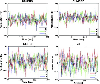
Figure 6. Position error of the user node (C2) according to three network-based collaborative algorithms and Kalman Filter (KF) (3-node case, in Figure 2b).
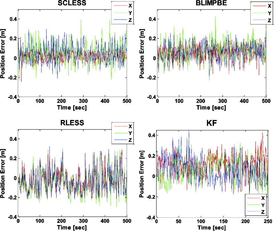
Figure 7. Position error of the user node (C2) according to three network-based collaborative algorithms and the Kalman Filter (KF) (5-node case, in Figure 2d).
5.1. Scenario 1: 3-Nodes in a Network
The added biases and random error in the user node's coordinates were significantly decreased from the simulated erratic coordinates, through the three network-based collaborative navigation algorithms, especially by the SCLESS, the BLIMPBE, the RLESS and the Kalman filter (see Figure 6). The SCLESS and BLIMPBE method showed better performance (especially in the standard deviation) than the RLESS and the Kalman filter. The RLESS and the Kalman filter showed the comparable biases, but the random errors were not adequately removed, as compared to the two other methods. The SCLESS and BLIMPBE solutions were almost the same for the user node, while the SCLESS solution absorbed the (added) biases into the network. Therefore, the estimated coordinates of user node in a network by using the a priori variance information were affected accordingly. Because RLESS is predominantly dependent on the accuracy of the coordinates to be fixed, it is not recommended for use in the network-based estimation. Table 1 shows the statistical results of the position difference between the original reference solutions and the estimated coordinates from the network-based algorithm, using the simulated biased data with random errors, as explained earlier.
Table 1. The statistical result of user node C2 of three network-based collaborative navigation algorithms and Kalman Filter (KF) solutions (3-node case).
5.2. Scenario 2: 5-Node Network
As can be seen in Figure 7 and Table 2 (statistical position error result of the user node C2), the SCLESS, the BLIMPBE, and the RLESS method performed better than the Kalman filter method because the increased number of reference nodes (i.e., inter-nodal distance measurements) can provide stronger geometry and redundancy of the proposed network-based collaborative navigation algorithms. The SCLESS method showed best standard deviations (also, in the Root Mean Square [RMS]) of the user node among all proposed estimation methods. Similarly to Scenario 1, the RLESS showed worse accuracy of the user nodes than that of other two network-based collaborative navigation algorithms.
Table 2. The statistical results of fifth user node C2 of three network-based collaborative navigation algorithms and Kalman Filter (KF) solutions (5-node network).
Overall, it can be seen that the proposed network-based collaborative algorithm methods can enhance the accuracy and the stability in the coordinate estimation of a user node by using only inter-nodal distance measurements when a GPS signal is not available. The methods and analysis presented in this paper provide a way to improve the solutions by simply building a network and applying these statistical collaborative navigation estimation methods. Although only inter-nodal range measurement is used in this study, additional ranging solutions and multi-sensor output could be applied to the network-based collaborative navigation case as well. The position errors RMS of SCLESS (BLIMPBE) were smaller by about 33% (32%) with respect to the Kalman filter results in Scenario 1. In Scenario 2, SCLESS, BLIMPBE and RLESS position errors were smaller that that of the Kalman filter by about 28%, 24%, and 9%, respectively. Even though the accuracy improvement achieved by using one of the statistical-based methods is at sub-decimetre level, which may not be relevant in land vehicle navigation, it has substantial relevance in navigating small platforms, such as swarms of autonomous miniature vehicles or robots.
6. CONCLUSIONS
It was demonstrated that the proposed statistical network-based ‘Collaborative Navigation’ algorithms can improve the position accuracy of the user node in the network based on field test data and simulated ranges. The ‘GPSVan’ and the ‘mobile cart’ with three geodetic GPS base stations were used in the field tests discussed here. Three network-based collaborative navigation algorithms, namely the Stochastic Constrained Least-Squares Solution (SCLESS), the Best Linear Minimum Partial Bias Estimation (BLIMPBE) and the Restricted Least-Squares Solution (RLESS) were proposed and compared to the Kalman filter to obtain accurate position of the user node and all other nodes in a network under realistic field conditions. The SCLESS method showed the best performance, especially, in the standard deviation, among the proposed ‘Network-based Estimation’ methods and the Kalman filter. In other proposed network-based estimation methods, the overall performance of the SCLESS and the BLIMPBE was better than that of the RLESS in the 5-node and 3-node cases. Therefore, it is concluded that the statistical collaborative navigation algorithm is a preferred estimation method for the collaborative navigation applications such as robots, ground-users and autonomous miniature vehicles.


