


1. Introduction
Adiabatic invariance historically played an essential role in the development of plasma physics, especially in the theory of charged-particle motion in strong magnetic fields. See Cary & Brizard (Reference Cary and Brizard2009) for an in-depth review of the latter topic. While an adiabatic invariant is not a true conserved quantity, it is approximately conserved over large intervals of time, and is therefore just as good as a true invariant for many practical purposes. In this article we will derive a new general formula for the adiabatic invariant associated with a nearly periodic Hamiltonian system. Such systems, along with their adiabatic invariants, were previously studied systematically in Kruskal (Reference Kruskal1962).
Today the most popular method for computing adiabatic invariants involves near-identity coordinate transformations. First ‘nice’ coordinates are found in which the expression for the adiabatic invariant becomes simple. Then the inverse coordinate transformation is applied to find an expression for the adiabatic invariant in a simpler, more desirable coordinate system. This approach is exemplified by Littlejohn's work on Hamiltonian formulations of guiding centre dynamics in Littlejohn (Reference Littlejohn1981, Reference Littlejohn1982, Reference Littlejohn1983, Reference Littlejohn and Marsden1984). Speaking more generally, at present there are (involved) procedures for computing adiabatic invariants, but general-use formulas for adiabatic invariants are unavailable.
The formula that we will obtain does not involve coordinate transformations. Instead it builds upon the coordinate-free ideas developed in Omohundro (Reference Omohundro1986) concerning the so-called roto-rate vector. The roto-rate vector was first introduced in Kruskal (Reference Kruskal1962) as a vector field  $\boldsymbol {R}$ that generates an approximate
  $U(1)$ (the group of complex numbers with unit modulus) symmetry for nearly periodic systems. Kruskal recognized the physical and conceptual significance of the roto-rate vector, but did not know how to compute
  $\boldsymbol {R}$ without first introducing an infinite sequence of near-identity coordinate transformations. Over twenty years later, Omohundro (Reference Omohundro1986) showed that, in principle,
  $\boldsymbol {R}$ can be computed in any coordinate system without introducing near-identity coordinate transformations, and even gave an algorithm for carrying out the calculation order by order in perturbation theory. However, Omohundro's results stop short of providing general formulas for
  $\boldsymbol {R}$, presumably as a result of the cumbersome nature of his algorithm.
Our approach to deriving a general formula for a nearly periodic Hamiltonian system's adiabatic invariant starts by improving Omohundro's algorithm for computing the roto-rate. The key to the improvement is recognizing that the messiest element of Omohundro's algorithm, namely enforcing that the integral curves of the roto-rate vector are  $2{\rm \pi}$-periodic, may be reimagined as a straightforward application of the famous Baker–Campbell–Hausdorff formula for the logarithm of composed exponentials. Using this improved algorithm we will push past Omohundro's results by deriving general-use, coordinate-independent formulas for the roto-rate. We will then feed these formulas into Noether's theorem for presymplectic Hamiltonian systems (see, e.g. Munteanu Reference Munteanu2013) in order to identify coordinate-independent formulas for the adiabatic invariant.
Our principal motivation for deriving this new formula is a desire for computing adiabatic invariants in infinite-dimensional Hamiltonian systems. While coordinate transform methods (e.g. perturbative changes of dependent variables) can be applied to such systems, the complexity of the required calculations easily gets out of hand. Coordinate-independent formulas for a system's adiabatic invariant would bypass much of this tedium, and therefore comprise a more efficient route to the desired result.
That said, we will not present any infinite-dimensional example applications in this article. Instead we will first use our new formula to reproduce the first two terms in the adiabatic invariant series for non-relativistic strongly magnetized charged particles. Then we will use our formula to calculate a coordinate-free expression for the field-line adiabatic invariant associated with a magnetic field whose lines of force are nearly closed. This adiabatic invariant defines approximate flux surfaces for this special class of magnetic fields, which includes near-axisymmetric-vacuum fields, and more generally any field that is close to an integrable field with constant rational rotational transform. It is worth remarking from the outset that this approximate flux function is not provided by standard Kolmogorov–Arnold–Moser (KAM) theory, which crucially relies on unperturbed fields with non-vanishing shear.
As we derive the general formula we will make liberal use of the standard machinery for performing calculus on manifolds, which includes Lie derivatives, flows, pullbacks, differential forms and Stokes’ theorem. A complete and rigorous description of this machinery, along with a vast amount of useful information concerning the coordinate-independent approach to Hamiltonian systems, is given in Abraham & Marsden (Reference Abraham and Marsden2008). The recent tutorial (MacKay Reference MacKay2020) on differential forms for plasma physicists is also an invaluable resource. Throughout the article we will adopt the notation  ${\unicode{x2A0F}} Q(\theta )\,\textrm {d}\theta = (2{\rm \pi} )^{-1}\int _0^{2{\rm \pi} }Q(\theta )\,\textrm {d}\theta$ for averages over an angular variable
  $\theta \in U(1)$.
The systems that exhibit the adiabatic invariants we would like to compute have two essential features: (a) they are nearly periodic, and (b) they possess a Hamiltonian structure. Property (a) ensures the existence of the roto-rate vector, which may be thought of as an approximate  $U(1)$-symmetry of the equations of motion. Property (b) enables the application of Noether's theorem to find an approximate conservation law, i.e. an adiabatic invariant, associated with this approximate symmetry. In order to explain and expand upon these points we will first discuss nearly periodic systems that are not necessarily Hamiltonian. In particular we will derive a coordinate-free formula for the roto-rate vector associated with such a system. This discussion will form the content of § 2. Then we will specialize to nearly periodic systems that happen to possess (presymplectic) Hamiltonian structure. This specialization will ultimately lead to the formulas for the adiabatic invariant series in § 3. As a way of illustrating the application of our formula we will use it in § 4 to compute the charged-particle adiabatic invariant, and again in § 5 to derive a field-line adiabatic invariant for magnetic fields with field lines that are nearly closed.
Readers who are interested in expressions for adiabatic invariants, but who are not interested in the derivation of such expressions may skip directly to Theorem 3.5. The relevant formulas are (3.14)–(3.17). Appendix A provides the details of how to work with these formulas using index notation.
2. Nearly periodic systems and the roto-rate vector
A nearly periodic system is a two time scale dynamical system whose short time scale dynamics is characterized by strictly periodic motion. Examples include masses conjoined by a stiff spring hung on the free end of a pendulum, and a charged particle in a strong magnetic field. For the sake of clarity the following definition of nearly periodic systems will be useful.
Definition 2.1 (Nearly periodic system) A nearly periodic system is a (possibly infinite-dimensional) ordinary differential equation of the form  $\dot {z} = \epsilon ^{-1}V_\epsilon (z)$ with the following properties.
(i) The vector field
 $V_\epsilon$ depends smoothly on $\epsilon$ in a neighbourhood of $0\in \mathbb {R}$.
(ii) The limiting vector field
$V_0 = \omega _0\xi _0$. Here $\xi _0$ is a vector field with integral curves that are strictly periodic with period $2{\rm \pi}$, and the frequency function $\omega _0$ is a smooth, positive function that is constant along $\xi _0$ integral curves.


Remark 2.2 While the frequency function is not allowed to pass through zero, the vector field  $\xi _0$ may do so. Therefore the limiting short time scale dynamics described by
  $V_0$ may have fixed points. In contrast, Kruskal (Reference Kruskal1962) requires that
  $V_0$ is nowhere vanishing. We have chosen to relax Kruskal's stronger assumption because his theory really only requires a non-vanishing frequency function. Moreover zeros of
  $V_0$ do occur in practice, and indicate the presence of a so-called slow manifold (cf. MacKay Reference MacKay, Dauxois, Litvak-Hinenzon, MacKay and Spanoudaki2004).
Away from the zeros of  $\xi _0$, nearly periodic systems exhibit a time scale separation that increases as
  $\epsilon$ tends to
  $0$. This suggests that averaging over the fast periodic motion described by
  $V_0$ ought to be permissible for small
  $\epsilon$. In more geometric terms, it is reasonable to expect that the equations of motion
  $\dot {z} = \epsilon ^{-1}V_\epsilon (z)$ defining a nearly periodic system possess an approximate
  $U(1)$-symmetry whose infinitesimal generator is given by
  $\xi _0$ to leading order in
  $\epsilon$.
If the equations of motion possessed a true  $U(1)$-symmetry then there would be a vector field
  $\xi _\epsilon$ on
  $z$-space, which we will call
  $Z$, with the following properties.
(a) The integral curves of
$\xi _\epsilon$, i.e. the solutions of the ordinary differential equation (ODE) $\dot {z} = \xi _\epsilon (z)$, must each be periodic with period $2{\rm \pi}$. Note that this condition does not preclude $\xi _\epsilon$ from having fixed points, which may be assigned any period. Nor does it rule out integral curves with period $2{\rm \pi} /n$, $n\in \mathbb {Z}$, which arise when the integral curves form a Seifert fibration. (See the appendix in Arnold (Reference Arnold1989).)(b) The flows of
$\xi _\epsilon$ and $V_\epsilon$ must commute. Equivalently, $[\xi _\epsilon ,V_\epsilon ] = 0$, where $[\cdot ,\cdot ]$ denotes the vector field commutator.


Such a  $\xi _\epsilon$ is referred to as the infinitesimal generator of a
  $U(1)$-symmetry.
Given a nearly periodic system the existence of such a  $\xi _\epsilon$ is typically too much to hope for. On the other hand it is always possible to find a formal power series,
 \[ \xi_\epsilon = \xi_0 + \epsilon \xi_1 + \epsilon^2 \xi_2 + \cdots, \]
whose coefficients  $\xi _k$ are vector fields on
  $Z$, and that satisfies the properties (a) and (b) to all orders in
  $\epsilon$. Such a formal power series is known as a roto-rate vector. Existence of a roto-rate vector is one way to precisely define the notion of approximate
  $U(1)$-symmetry.
Definition 2.3 Given a vector field  $U$ on a manifold
  $Z$ with integral curves that exist for all time, the exponential of
  $U$ is the unique mapping
  $\exp (U):Z\rightarrow Z$ such that
  $\exp (U)(z) = z(1)$, where
  $z(t)$ is the solution of
  $\dot {z} = U(z)$ with
  $z(0) = z$. If
  $\phi :Z\rightarrow Z$ is a map and there is some vector field
  $W$ such that
  $\phi =\exp (W)$ then we write
  $W = \ln (\phi )$ and say
  $W$ is a logarithm of
  $\phi$.
Remark 2.4 There may be several logarithms of a map  $\phi$, or none at all. For smooth families of mappings
  $\phi _\lambda$,
  $\lambda \in \mathbb {R}$, with
  $\phi _0 = \text {id}_Z$,
  $\ln (\phi _\lambda )$ may be defined uniquely as a formal power series in
  $\lambda$.
Definition 2.5 (Roto-rate vector) Given a nearly periodic system  $\dot {z} = \epsilon ^{-1}V_\epsilon (z)$, a roto-rate vector is a formal power series
  $\xi _\epsilon = \xi _0 + \epsilon \xi _1 + \epsilon ^2 \xi _2 + \cdots$ with vector field coefficients such that
  $\xi _0 = V_0/\omega _0$ and
(i)
$[\xi _\epsilon ,V_\epsilon ] = 0$;(ii)
$\ln (\exp (-2{\rm \pi} \,\xi _0)\circ \exp (2{\rm \pi} \,\xi _\epsilon )) = 0$;


where the previous two equalities are understood in the sense of formal power series.
Remark 2.6 The integral curves of a vector field  $\xi _\epsilon$ will be
  $2{\rm \pi}$-periodic if and only if the exponential
  $\exp (2{\rm \pi} \xi _\epsilon )$ is equal to the identity map on
  $z$-space. If
  $\xi _0$ happens to already have this property then it must be the case that
  $\text {id}_Z = \exp (2{\rm \pi} \,\xi _0)\circ \exp (-2{\rm \pi} \xi _0)\circ \exp (2{\rm \pi} \xi _\epsilon ) = \exp (-2{\rm \pi} \xi _0)\circ \exp (2{\rm \pi} \xi _\epsilon ).$ By the Baker–Campbell–Hausdorff (BCH) formula there is a formal power series vector field
  $Z_\epsilon$ such that
 \[ \exp(Z_\epsilon) = \exp(-2{\rm \pi}\xi_0)\circ\exp(2{\rm \pi}\xi_\epsilon), \]
i.e.  $Z_\epsilon = \ln (\exp (-2{\rm \pi} \xi _0)\circ \exp (2{\rm \pi} \xi _\epsilon ))$. Because
  $\xi _0$ is
  $\epsilon$-close to
  $\xi _\epsilon$
  $Z_\epsilon$ must be
  $\epsilon$-small. The only formal power series
  $Z_\epsilon = Z_0 + \epsilon Z_1 + \cdots$ that is
  $\epsilon$-small and that formally exponentiates to the identity is
  $Z_\epsilon = 0$. This explains the second property in the definition.
Roto-rate vectors are remarkable due to the following.
Theorem 2.7 (Existence and uniqueness of the roto-rate vector) Given a nearly periodic system  $\dot {z} = \epsilon ^{-1} V_\epsilon (z)$ with
  $V_0 = \omega _0\xi _0$ there is a unique roto-rate vector
  $\xi _\epsilon$.
Proof. This result follows from minor modifications of the arguments in Kruskal (Reference Kruskal1962), which does not allow  $\xi _0$ to have fixed points. Therefore we will only outline the main steps in the proof.
The first step is show that there is a (non-unique) formally defined near-identity diffeomorphism  $T_\epsilon :Z\rightarrow Z$ such that
  $\bar {V}_\epsilon = (T_\epsilon )_*V_\epsilon$ takes the form
  $\bar {V}_\epsilon = \bar {\omega }_\epsilon \,\xi _0 + \epsilon \delta \bar {V}_\epsilon$, where
  ${\mathcal {L}}_{\xi _0}\bar {\omega }_\epsilon = 0$ and
  $[\xi _0,\delta \bar {V}_\epsilon ] = 0$. Note that (formally) pulling back this expression for
  $\bar {V}_\epsilon$ along
  $T_\epsilon$ implies
  $V_\epsilon = \omega _\epsilon \,\xi _\epsilon + \epsilon \,\delta V_\epsilon$, where
  $\omega _\epsilon = T^*_\epsilon \bar {\omega }_\epsilon$,
  $\xi _\epsilon = T_\epsilon ^*\xi _0$ and
  $\delta V_\epsilon = T_\epsilon ^*\bar {V}_\epsilon$. This establishes the existence of at least one roto-rate vector because
  $\xi _\epsilon$ apparently has
  $2{\rm \pi}$-periodic integral curves, satisfies
  $\xi _0 = \xi _0$, and
 \[ [\xi_\epsilon, V_\epsilon] = {\mathcal{L}}_{\xi_\epsilon}(\omega_\epsilon\xi_\epsilon) + \epsilon {\mathcal{L}}_{\xi_\epsilon}\delta V_\epsilon = 0. \]
A procedure for finding the diffeomorphism  $T_\epsilon$ is the most commonly quoted result from Kruskal (Reference Kruskal1962). The reason the procedure still works when
  $\xi _0$ has fixed points is that solvability of the differential equations defining
  $T_\epsilon$ only requires periodicity of the
  $\xi _0$-flow and
  $\omega _{0}$ to be nowhere vanishing.
The second step is to show that if  $\xi _\epsilon ^\prime$ is any other roto-rate vector field then
  $\xi _\epsilon ^\prime = \xi _\epsilon$. While it is less well-known, this argument is also contained in Kruskal (Reference Kruskal1962). It proceeds along the following lines. Let
  $\bar {\xi }_\epsilon ^\prime = T_{\epsilon *}\xi _\epsilon ^\prime$. Introduce the decomposition
  $\bar {\xi }_\epsilon ^\prime = \langle \bar {\xi }_\epsilon ^\prime \rangle + (\bar {\xi }_\epsilon ^\prime )^{\textrm {osc}}$, where
  $\langle \bar {\xi }_\epsilon ^\prime \rangle = (2{\rm \pi} )^{-1}\int _0^{2{\rm \pi} } \exp (\theta \,\xi _0)^*\bar {\xi }_\epsilon \,\textrm {d}\theta$. Because
  $[\bar {\xi }_\epsilon ^\prime ,\bar {V}_\epsilon ]=0$ it must also be the case that
  $[(\bar {\xi }_\epsilon ^\prime )^{\textrm {osc}},\bar {V}_\epsilon ]=0$, which in turn is equivalent to the sequence of conditions
 \begin{gather} [(\bar{\xi}_0^\prime)^{\textrm{osc}},\omega_0 \xi_0] = 0, \end{gather}
 \begin{gather}\begin{array}{c}[(\bar{\xi}_1^\prime)^{\textrm{osc}},\omega_0 \xi_0] +[(\bar{\xi}_0^\prime)^{\textrm{osc}}, \bar{V}_1] = 0,\\ \ldots \end{array}\end{gather}
The first condition (2.1) is satisfied if and only if  $(\bar {\xi }_0^\prime )^{\textrm {osc}} = 0$. Substituting this in the second condition (2.2) therefore implies
  $[(\bar {\xi }_1^\prime )^{\textrm {osc}},\omega _0\xi _0] = 0$, which requires
  $(\bar {\xi }_1^\prime )^{\textrm {osc}} = 0$. This pattern continues to all orders in
  $\epsilon$ and shows that
  $(\bar {\xi }_\epsilon ^\prime )^{\textrm {osc}}=0$. Now the argument may be completed as follows. Because
  $\bar {\xi }_\epsilon ^\prime = \langle \bar {\xi }_\epsilon ^\prime \rangle$ is
  $S^1$-invariant the difference
  $\bar {\xi }_\epsilon ^\prime -\xi _0$ must also be
  $S^1$-invariant. Moreover because
  $\bar {\xi }_\epsilon ^\prime$ and
  $\xi _0$ agree when
  $\epsilon =0$ there must be an
  $S^1$-invariant
  $O(1)$ vector field
  $w_\epsilon$ such that
  $\bar {\xi }_\epsilon ^\prime - \xi _0 = \epsilon w_\epsilon$. Therefore
  $\exp (2{\rm \pi} \bar {\xi }_\epsilon ^\prime ) = \exp (2{\rm \pi} \xi _0 +2{\rm \pi} \epsilon w_\epsilon ) = \exp (2{\rm \pi} \xi _0)\circ \exp (2{\rm \pi} \epsilon w_\epsilon ) = \exp (2{\rm \pi} \epsilon w_\epsilon ) = \text {id}_Z$ in order for the integral curves of
  $\bar {\xi }_\epsilon ^\prime$ to each be
  $2{\rm \pi}$-periodic. (Note that we have made use of the commutativity
  $[\xi _0, w_\epsilon ] = 0$.) This identity may only be satisfied if
  $w_\epsilon =0$.
The preceding Theorem establishes the useful fact that by expanding the pair of conditions from Definition 2.5 in power series it should be possible to find the coefficients of the expansion  $\xi _\epsilon = \xi _0 + \epsilon \xi _1 + \cdots$ order-by-order. We will now follow this line of reasoning to derive explicit formulas for
  $\xi _0,\xi _1,\xi _2$, and
  $\xi _3$ in terms of Fourier harmonics of
  $V_\epsilon$ relative to
  $\xi _0$.
As a preparatory step we will establish the following variant of the BCH formula that is well suited to perturbation theory in  $\epsilon$.
Lemma 2.8 (Perturbative BCH formula) Let  $A$ and
  $B$ be vector fields on the manifold
  $Z$ and
  $\epsilon$ a small real parameter. The logarithm
  $Z_\epsilon = \ln (\exp (-A)\circ \exp (A+\epsilon B))$ exists as a formal power series in
  $\epsilon$,
  $Z_\epsilon = Z_0 + \epsilon Z_1 + \epsilon ^2 Z_2 + \cdots$. The formulas
 \begin{gather} Z_0 = 0, \end{gather}
 \begin{gather}Z_1 =\int_0^1 B_{\tau_1}\textrm{d}\tau_1, \end{gather}
 \begin{gather}Z_2 = \frac{1}{2}\int_0^1\int_0^{\tau_1}[B_{\tau_2},B_{\tau_1}]\,\textrm{d}\tau_2\,\textrm{d}\tau_1, \end{gather}
 \begin{gather}Z_3 = \frac{1}{6}\int_0^1\int_0^{\tau_1}\int_0^{\tau_2}( [B_{\tau_3},[B_{\tau_2},B_{\tau_1}]] + [[B_{\tau_3},B_{\tau_2}],B_{\tau_1}])\,\textrm{d}\tau_3\,\textrm{d}\tau_2\,\textrm{d}\tau_1, \end{gather}
with  $B_\tau = \exp (\tau A)^* B$, give the first few coefficients
  $Z_k$. More generally
 \begin{equation} Z_\epsilon = \epsilon \int_0^1\psi\left(\exp(\lambda {\mathcal{L}}_{A+\epsilon B})\exp(-\lambda{\mathcal{L}}_A)\right) \exp(\lambda A)^*B\,\textrm{d}\lambda,\end{equation}
with  $\psi (z) = z\ln z/(z-1)$, gives
  $Z_\epsilon$ to all orders in
  $\epsilon$.
Proof. The proof proceeds by first solving a seemingly more-difficult problem, namely finding an asymptotic series representation for  $Z_{\epsilon ,\lambda } = \ln (\exp (-\lambda A)\circ \exp (\lambda [A+\epsilon B]))$. To that end, first consider the
  $\lambda$-derivative of
  $\exp (Z_{\epsilon ,\lambda }) = \exp (-\lambda A)\circ \exp (\lambda [A+\epsilon B])$,
 \begin{align*} \partial_\lambda\exp(Z_{\epsilon,\lambda}) &= - A\circ \exp(Z_{\epsilon,\lambda}) + T\exp(-\lambda A)\circ [A+\epsilon B]\circ\exp(\lambda [A+\epsilon B])\\ & = (-A + \exp(\lambda A)^*[A+\epsilon B])\circ \exp(Z_{\epsilon,\lambda}). \end{align*}
In other words
 \begin{equation} \partial_\lambda\exp(Z_{\epsilon,\lambda}) \circ \exp(-Z_{\epsilon,\lambda}) = \epsilon \exp(\lambda A)^* B.\end{equation}
We will eventually obtain (2.7) by integrating (2.8) in  $\lambda$, but first we need an expression for
  $\partial _\lambda \exp (Z_{\epsilon ,\lambda }) \circ \exp (-Z_{\epsilon ,\lambda })$ in terms of
  $\partial _\lambda Z_{\epsilon ,\lambda }$. One way to find such an expression is the following. Let
  $C_\lambda$ be any
  $\lambda$-dependent vector field and set
  $\psi _{s,\lambda } = \exp (sC_\lambda )$. By the equality of mixed partials the vector fields
  $V_{s,\lambda } = \partial _\lambda \psi _{s,\lambda }\circ \psi _{s,\lambda }^{-1}$ and
  $\xi _{s,\lambda } = \partial _s \psi _{s,\lambda }\circ \psi _{s,\lambda }^{-1} = C_\lambda$ must be related by the condition
 \begin{equation} \partial_s V_{s,\lambda} + {\mathcal{L}}_{C_\lambda} V_{s,\lambda} = \partial_\lambda C_\lambda. \end{equation}
Thinking of the last condition as a differential equation for  $V_{s,\lambda }$, it can be solved using the method of variation of parameters. The solution for
  $V_{s,\lambda }$ is given by
 \begin{equation} V_{s,\lambda} = \exp(-s C_\lambda)^*\int_0^s \exp(\bar{s} C_\lambda)^*\partial_\lambda C_\lambda\,\textrm{d}\bar{s}.\end{equation}
Because  $V_{1,\lambda } = \partial _\lambda \psi _{1,\lambda }\circ \psi _{1,\lambda }^{-1} = \partial _\lambda \exp (C_\lambda )\circ \exp (-C_\lambda )$ (2.10) implies the general formula
 \begin{align} \partial_\lambda\exp(C_\lambda)\circ \exp(-C_\lambda) &= \exp(- C_\lambda)^* \int_0^1 \exp(\bar{s} C_\lambda)^*\partial_\lambda C_\lambda\,\textrm{d}\bar{s}\nonumber\\ & = \phi(-{\mathcal{L}}_{C_\lambda}) \partial_\lambda C_\lambda, \end{align}
where  $\phi (z) = [\exp (z) - 1]/z$. Applying this formula to (2.8) then gives
 \begin{equation} \begin{aligned} & \phi(-{\mathcal{L}}_{Z_{\epsilon,\lambda}}) \partial_\lambda Z_{\epsilon,\lambda} = \epsilon \exp(\lambda A)^* B,\\ \Rightarrow & \partial_\lambda Z_{\epsilon,\lambda}=\epsilon\frac{1}{\phi(-{\mathcal{L}}_{Z_{\epsilon,\lambda}})} \exp(\lambda A)^* B,\\ \Rightarrow & Z_{\epsilon,\lambda} = \int_0^{\lambda}\epsilon\frac{1}{\phi(-{\mathcal{L}}_{Z_{\epsilon,\bar{\lambda}}})} \exp(\bar{\lambda} A)^* B\,\textrm{d}\bar{\lambda}. \end{aligned} \end{equation}
While (2.12) may not seem helpful because  $Z_{\epsilon ,\lambda }$ appears under the integral sign, in fact it implies (2.7) for the following reason. Because
 \[ \exp({\mathcal{L}}_{Z_{\epsilon,\lambda}}) = (\exp(-\lambda A)\circ \exp(\lambda[A+\epsilon B]))^* = \exp(\lambda {\mathcal{L}}_{A+\epsilon B})\exp(-\lambda {\mathcal{L}}_{A}), \]
the Lie derivative  ${\mathcal {L}}_{Z_{\epsilon ,\lambda }}$ may be written
 \[ {\mathcal{L}}_{Z_{\epsilon,\lambda}} = \ln\left(\exp(\lambda {\mathcal{L}}_{A+\epsilon B})\exp(-\lambda {\mathcal{L}}_{A})\right). \]
If  $a \equiv \exp (\lambda {\mathcal {L}}_{A+\epsilon B})\exp (-\lambda {\mathcal {L}}_{A})$ it therefore follows that
 \begin{align} \frac{1}{\phi(-{\mathcal{L}}_{Z_{\epsilon,\lambda}})} &= \frac{1}{\phi(-\ln a)}\nonumber\\ & = -\frac{\ln a}{\exp(-\ln a) - 1}\nonumber\\ & = \psi(a). \end{align}
Substituting (2.13) in (2.12) gives (2.7), as desired.
In order to obtain the formulas (2.3)–(2.6) it is sufficient to expand the formal expression (2.7) as a power series in  $\epsilon$. This rather tedious calculation proceeds as follows. First it is useful to find the power series expansion of the operator
  $a_{\epsilon ,\lambda } = \exp (\lambda {\mathcal {L}}_{A+\epsilon B})\exp (-\lambda {\mathcal {L}}_{A})$. Let
  $f:Z\rightarrow \mathbb {R}$ be any scalar on
  $Z$ and introduce
  $f_\lambda = \exp (\lambda {\mathcal {L}}_{A+\epsilon B}) f$. The scalar
  $f_\lambda$ obeys the differential equation
  $\partial _\lambda f_\lambda = {\mathcal {L}}_{A+\epsilon B} f_\lambda$. Introducing the variation-of-parameters ansatz
  $f_\lambda = \exp (\lambda {\mathcal {L}}_{A})\bar {f}_\lambda$, the scalar
  $\bar {f}_\lambda$ therefore satisfies
  $\partial _\lambda \bar {f}_\lambda = \epsilon {\mathcal {L}}_{\exp (-\lambda A)^* B}\bar {f}_\lambda$, or in integral form
 \begin{align} \bar{f}_\lambda &= f + \epsilon\int_0^\lambda {\mathcal{L}}_{B_{-s_1}}\bar{f}_{s_1}\,\textrm{d} s_1\nonumber\\ & = f+ \epsilon \int_0^\lambda {\mathcal{L}}_{B_{-s_1}}f\,\textrm{d} s_1 + \epsilon^2\int_0^\lambda\int_0^{s_1}{\mathcal{L}}_{B_{-s_1}}{\mathcal{L}}_{B_{-s_2}}f\,\textrm{d} s_2\,\textrm{d} s_1 + O(\epsilon^3), \end{align}
where we have introduced the shorthand notation  $B_{s} = \exp (s A)^* B$. This shows that
  $a_{\epsilon ,\lambda }$ has the asymptotic expansion
 \[ a_{\epsilon,\lambda} = \exp(\lambda {\mathcal{L}}_A)\left(1 + \epsilon \bar{a}_{1,\lambda} + \epsilon^2 \bar{a}_{2,\lambda} + \cdots\right)\exp(-\lambda {\mathcal{L}}_A), \]
where
 \begin{gather} \bar{a}_{1,\lambda} = \int_0^\lambda {\mathcal{L}}_{B_{-s_1}}\textrm{d} s_1, \end{gather}
 \begin{gather}\bar{a}_{2,\lambda} = \int_0^\lambda\int_0^{s_1}{\mathcal{L}}_{B_{-s_1}}{\mathcal{L}}_{B_{-s_2}}\textrm{d} s_2\,\textrm{d} s_1. \end{gather}
Combining this observation with the series representation of  $\psi (1 + x) = 1 + \frac {1}{2}x - \frac {1}{6} x^2 + \frac {1}{12}x^3 + \cdots$ therefore implies
 \begin{equation} Z_0 = 0, \end{equation}
 \begin{equation}Z_1 = \int_0^1 \exp(\lambda A)^*B\,\textrm{d}\lambda = \int_0^1 \exp(\tau_1 A)^*B\,\textrm{d}\tau_1, \end{equation}
 \begin{align} Z_2 &= \frac{1}{2}\int_0^1 \exp(\lambda A)^* \bar{a}_{1,\lambda}B\,\textrm{d}\lambda = \frac{1}{2}\int_0^1\int_0^\lambda \exp(\lambda A)^*[B_{-s_1},B]\,\textrm{d} s_1\,\textrm{d}\lambda\nonumber\\ &= \frac{1}{2}\int_0^1\int_0^{\tau_1}[B_{\tau_2},B_{\tau_1}]\,\textrm{d}\tau_2\,\textrm{d}\tau_1, \end{align}
 \begin{gather} Z_3 = -\frac{1}{6}\int_0^1 \exp(\lambda A)^* \bar{a}_{1,\lambda}^2 B\,\textrm{d}\lambda + \frac{1}{2}\int_0^1 \exp(\lambda A)^* \bar{a}_{2,\lambda}B\,\textrm{d}\lambda. \end{gather}
These expressions for  $Z_0,Z_1,Z_2$ clearly reproduce (2.3)–(2.5). To see that (2.20) reproduces (2.6) notice first that
 \begin{align} Z_3 & = -\frac{1}{6}\int_0^1 \exp(\lambda A)^*\int_0^\lambda\int_0^\lambda[ B_{-s_1},[B_{-s_2},B]]\,\textrm{d} s_2\,\textrm{d} s_1\,\textrm{d}\lambda\nonumber\\ & \quad+ \frac{1}{2}\int_0^1 \exp(\lambda A)^* \int_0^\lambda\int_0^{s_1}[B_{-s_1}[B_{-s_2},B]]\,\textrm{d} s_2\,\textrm{d} s_1\,\textrm{d}\lambda. \end{align}
Next, observe that if  $g(s_1,s_2) = [B_{-s_1},[B_{-s_2},B]]$ then by Fubini's theorem
 \begin{equation} \int_0^\lambda\int_0^\lambda g(s_1,s_2)\,\textrm{d} s_2\,\textrm{d} s_1 = \int_0^\lambda\int_0^{s_1} g(s_1,s_2)\,\textrm{d} s_2\,\textrm{d} s_1 +\int_0^\lambda\int_0^{s_1} g(s_2,s_1)\,\textrm{d} s_2\,\textrm{d} s_1. \end{equation}
It follows that
 \begin{align*} Z_3 & = -\frac{1}{6}\int_0^1 \exp(\lambda A)^*\int_0^\lambda\int_0^{s_1}([ B_{-s_1},[B_{-s_2},B]] +[ B_{-s_2},[B_{-s_1},B]] )\,\textrm{d} s_2\,\textrm{d} s_1\,\textrm{d}\lambda\\ & \quad+ \frac{1}{2}\int_0^1 \exp(\lambda A)^* \int_0^\lambda\int_0^{s_1}[B_{-s_1}[B_{-s_2},B]]\,\textrm{d} s_2\,\textrm{d} s_1\,\textrm{d}\lambda\\ &= \int_0^1\int_0^\lambda\int_0^{s_1}\exp(\lambda A)^* \left(\frac{1}{3}[ B_{-s_1},[B_{-s_2},B]] - \frac{1}{6}[ B_{-s_2},[B_{-s_1},B]]\right)\,\textrm{d} s_2\,\textrm{d} s_1\,\textrm{d}\lambda\\ & = \int_0^1\int_0^\lambda\int_0^{s_1}\exp(\lambda A)^* \left(\frac{1}{6}[ B_{-s_1},[B_{-s_2},B]] + \frac{1}{6}[[B_{-s_1}, B_{-s_2}],B]]\right)\,\textrm{d} s_2\,\textrm{d} s_1\,\textrm{d}\lambda\\ & = \frac{1}{6}\int_0^1\int_0^{\tau_1}\int_0^{\tau_2}( [B_{\tau_3},[B_{\tau_2},B_{\tau_1}]] + [[B_{\tau_3},B_{\tau_2}],B_{\tau_1}])\,\textrm{d}\tau_3\,\textrm{d}\tau_2\,\textrm{d}\tau_1, \end{align*}
where we have applied the Jacobi identity  $[B_{-s_2},[B_{-s_1},B]] = [[B_{-s_2},B_{-s_1}],B] + [B_{-s_1},[B_2,B]]$ on the second-to-last line, and we changed integration variables to
  $\tau _1 = \lambda$,
  $\tau _3 = \lambda - s_1$, and
  $\tau _2 = \lambda - s_2$ on the last line.
With the modified BCH formula from Lemma 2.8 in hand it is now straightforward to derive formulas for the coefficients of  $\xi _\epsilon = \xi _0 +\epsilon \,\xi _1 + \epsilon ^2\,\xi _2 + \cdots$ as follows.
Definition 2.9 (Mean and oscillating subspaces) Given a nearly periodic system with roto-rate vector  $\xi _\epsilon$, the space of limiting mean vector fields
  $\langle \mathfrak {X}(Z)\rangle$ or just mean vector fields for short is the subspace of vector fields
  $A$ on
  $Z$ that are equal to their
  $U(1)$-average along
  $\xi _0$. In symbols
  $A\in \langle \mathfrak {X}(Z)\rangle$ means
  $A =\langle A\rangle (2{\rm \pi} )^{-1}\int _0^{2{\rm \pi} } \exp (\theta \,\xi _0)^*A\,\textrm {d}\theta$. The space of limiting oscillating vector fields
  $\mathfrak {X}(Z)^{\textrm {osc}}$, or just oscillating vector fields for short, is the subspace of vector fields on
  $Z$ that average to zero along
  $\xi _0.$ That is,
  $A\in \mathfrak {X}(Z)^{\textrm {osc}}$ if
  $\langle A\rangle = 0$.
Remark 2.10 Standard results on Fourier series imply that the mean and fluctuating subspaces are complementary subspaces of  $\mathfrak {X}(Z)$, the space of vector fields on
  $Z$. A projection onto
  $\langle \mathfrak {X}(Z)\rangle$ is
  $\bar {{\rm \pi} }: A\mapsto \langle A\rangle$ and a projection onto
  $\mathfrak {X}(Z)^{\textrm {osc}}$ is
  $\tilde {{\rm \pi} } = 1 - \bar {{\rm \pi} }$. If
  $A$ is any vector field on
  $Z$ then the notations
  $A = \langle A\rangle + A^{\mathrm {osc}}$ and
  $A = \langle A\rangle +\tilde {A}$ will be used interchangeably to denote the decomposition of
  $A$ into its mean,
  $\langle A\rangle = \bar {{\rm \pi} }A$, and fluctuating parts,
  $A^{\mathrm {osc}} = \tilde {A} = \tilde {{\rm \pi} }A$.
Theorem 2.11 (Formula for the roto-rate vector) The first four coefficients of the roto-rate vector  $\xi _\epsilon$ associated with a nearly periodic system
  $\dot {z} = \epsilon ^{-1}V_\epsilon (z)$ are given in terms of the power series expansion of
  $V_\epsilon = \omega _0 \xi _0 + \epsilon V_1 + \epsilon ^2 V_2 + \cdots$ as follows.
 \begin{equation} \xi_0 = V_0/\omega_0, \end{equation}
 \begin{equation}\xi_1 = {\mathcal{L}}_{\xi_0} I_0\tilde{V}_1, \end{equation}
 \begin{equation}\xi_2 = {\mathcal{L}}_{\xi_0} I_0\tilde{V}_2 + {\mathcal{L}}_{\xi_0} I_0[ I_0\tilde{V}_1, \langle V_1\rangle] + \frac{1}{2}{\mathcal{L}}_{\xi_0} I_0[I_0\tilde{V}_1,\tilde{V}_1]^{\textrm{osc}} + \frac{1}{2}[{\mathcal{L}}_{\xi_0} I_0\tilde{V}_1, I_0\tilde{V}_1], \end{equation}
 \begin{align} \xi_3 &= {\mathcal{L}}_{\xi_0}\left(I_0\tilde{V}_3 + I_0[ I_0\tilde{V}_1,\langle V_2\rangle]^{\textrm{osc}} +I_0[ I_0\tilde{V}_2,\langle V_1\rangle]^{\textrm{osc}}\vphantom{\frac{1}{2}}\right.\nonumber\\ &\quad +\frac{1}{2} I_0[I_0\tilde{V}_2,\tilde{V}_1]^{\textrm{osc}}+ \frac{1}{2}I_0[I_0\tilde{V}_1,\tilde{V}_2]^{\textrm{osc}}+\frac{1}{3}I_0[I_0\tilde{V}_1,[I_0\tilde{V}_1,\tilde{V}_1]]^{\textrm{osc}}\nonumber\\ &\quad+I_0[ I_0[ I_0\tilde{V}_1, \langle V_1\rangle],\langle V_1\rangle] + \frac{1}{2}I_0[ I_0[I_0\tilde{V}_1,\tilde{V}_1]^{\textrm{osc}},\langle V_1\rangle]\nonumber\\ &\quad\left.+\frac{1}{2}I_0[I_0\tilde{V}_1,[I_0\tilde{V}_1,\langle V_1\rangle]]^{\textrm{osc}}\right)\nonumber\\ &\quad + \frac{1}{2} [{\mathcal{L}}_{\xi_0} I_0 \tilde{V}_1,I_0\tilde{V}_2]+ \frac{1}{2} [{\mathcal{L}}_{\xi_0} I_0 \tilde{V}_2,I_0\tilde{V}_1]\nonumber\\ &\quad +[I_0[{\mathcal{L}}_{\xi_0} I_0\tilde{V}_1,{V}_1]^{\textrm{osc}},I_0\tilde{V}_1]+I_0[\langle [{\mathcal{L}}_{\xi_0} I_0\tilde{V}_1,\tilde{V}_1]\rangle, I_0\tilde{V}_1]\nonumber\\ &\quad +\frac{1}{3}[I_0\tilde{V}_1,[{\mathcal{L}}_{\xi_0} I_0\tilde{V}_1,I_0\tilde{V}_1]]. \end{align}
Here,  $I_0$ is the inverse of
  ${\mathcal {L}}_{V_0}$ restricted to the fluctuating subspace regarded as a linear map
  $\mathfrak {X}^{\mathrm {osc}}(Z)\rightarrow \mathfrak {X}^{\mathrm {osc}}(Z)$.
Proof. The proof proceeds by directly analysing the conditions in Definition 2.5 order-by-order in  $\epsilon$. First Lemma 2.8 will be applied with
  $A = 2{\rm \pi} \xi _0$ and
  $B = 2{\rm \pi} (\xi _1 + \epsilon \xi _2 + \epsilon ^2 \xi _3 + \cdots )$ in order to identify the coefficients of the formal power series
 \[ Z_{\epsilon} = \ln \left(\exp(-2{\rm \pi}\xi_0)\circ\exp(2{\rm \pi}\xi_\epsilon)\right). \]
Then the power series coefficients of  $[\xi _\epsilon ,V_\epsilon ]$ and
  $Z_\epsilon$ will each be set equal to zero.
After changing integration variables from  $\tau _k$ to
  $\theta _k = 2{\rm \pi} \tau _k$ and accounting for the fact that
  $B = 2{\rm \pi} (\xi _1 + \epsilon \xi _2 + \epsilon ^2 \xi _3 + \cdots )$ is itself a formal power series, the first several coefficients of
  $Z_\epsilon$ given by Lemma 2.8 are
 \begin{gather} Z_0 = 0, \end{gather}
 \begin{gather}Z_1 =2{\rm \pi} \langle \xi_1\rangle, \end{gather}
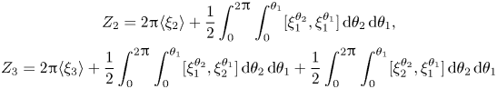 \begin{gather}Z_2 = 2{\rm \pi} \langle \xi_2\rangle+\frac{1}{2}\int_0^{2{\rm \pi}}\int_0^{\theta_1}[\xi_1^{\theta_2},\xi_1^{\theta_1}]\,\textrm{d}\theta_2\,\textrm{d}\theta_1, \\ Z_3 = 2{\rm \pi} \langle \xi_3\rangle+\frac{1}{2}\int_0^{2{\rm \pi}}\int_0^{\theta_1}[\xi_1^{\theta_2},\xi_2^{\theta_1}]\,\textrm{d}\theta_2\,\textrm{d}\theta_1+ \frac{1}{2}\int_0^{2{\rm \pi}}\int_0^{\theta_1}[\xi_2^{\theta_2},\xi_1^{\theta_1}]\,\textrm{d}\theta_2\,\textrm{d}\theta_1 \nonumber \end{gather}
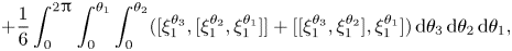 \begin{gather}+\frac{1}{6}\int_0^{2{\rm \pi}}\int_0^{\theta_1}\int_0^{\theta_2}( [\xi_1^{\theta_3},[\xi_1^{\theta_2},\xi_1^{\theta_1}]] + [[\xi_1^{\theta_3},\xi_1^{\theta_2}],\xi_1^{\theta_1}])\,\textrm{d}\theta_3\,\textrm{d}\theta_2\,\textrm{d}\theta_1, \end{gather}
where  $\xi _k^{\theta _j} = \exp (\theta _j\,\xi _0)^*\xi _k$. Each of these coefficients must vanish, but we will not examine the consequences of this vanishing now. Instead we will examine the vanishing of the
  $Z_k$ and the coefficients of
  $[\xi _\epsilon ,V_\epsilon ]$ incrementally and simultaneously in the following paragraphs.
The  $O(1)$ coefficients of the series
  $Z_\epsilon$ and
  $[\xi _\epsilon ,V_\epsilon ]$ are given by (2.27) and
  $[\xi _0,V_0]$, respectively. The former is obviously zero, while the latter vanishes because
  ${\mathcal {L}}_{\xi _0}\omega _0 = 0$. Thus no constraints are placed on the
  $\xi _k$ at this order. Note that
  $\xi _0 = V_0/\omega _0$ by definition of the roto-rate vector.
The  $O(\epsilon )$ coefficients of
  $Z_\epsilon$ and
  $[\xi _\epsilon ,V_\epsilon ]$ are given by (2.28) and
  $[\xi _0,V_1] + [\xi _1,V_0]$, respectively. Vanishing of these coefficients is equivalent to the joint satisfaction of the three conditions
 \begin{gather} 0 = \langle \xi_1 \rangle, \end{gather}
 \begin{gather}0 = [\xi_0,V_1] + [\xi_1,V_0]^{\textrm{osc}}, \end{gather}
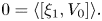 \begin{gather}0 = \langle [\xi_1,V_0] \rangle. \end{gather}
We claim that the conditions (2.31) and (2.32) uniquely determine  $\xi _1$, and that when
  $\xi _1$ is so determined the condition (2.33) is satisfied automatically. As for the first part of our claim, notice that condition (2.32) is equivalent to the linear equation
  ${\mathcal {L}}_{V_0}\tilde {\xi }_1 = {\mathcal {L}}_{\xi _0} \tilde {V}_1$, which has the unique solution
  $\tilde {\xi }_1 = {\mathcal {L}}_{\xi _0} I_0\tilde {V}_1$. Because condition (2.31) says that
  $\xi _1$ has zero average, the last observation implies that in fact
  $\xi _1 = {\mathcal {L}}_{\xi _0} I_0\tilde {V}_1$, which is precisely the desired formula (2.24). As for the second part of our claim, it is enough to observe that, because
  $\xi _1 = \tilde {\xi }_1$,
  $\langle [\xi _1,V_0] \rangle = \langle [\widetilde {\xi _1},V_0] \rangle = [\langle \tilde {\xi }_1\rangle , V_0] = 0$.
The  $O(\epsilon ^2)$ coefficients of
  $Z_\epsilon$ and
  $[\xi _\epsilon , V_\epsilon ]$ are given by (2.28) and
  $[\xi _0,V_2] + [\xi _1,V_1] + [\xi _2,V_0]$, respectively. Vanishing of these coefficients is equivalent to
 \begin{gather} 0 = \langle \xi_2\rangle+{\frac{1}{2}}{\unicode{x2A0F}} \int_0^{\theta_1}[\xi_1^{\theta_2},\xi_1^{\theta_1}]\,\textrm{d}\theta_2\,\textrm{d}\theta_1, \end{gather}
 \begin{gather}0 = [\xi_0,V_2] + [\xi_1,V_1]^{\textrm{osc}} + [\xi_2,V_0]^{\textrm{osc}}, \end{gather}
 \begin{gather}0 = \langle [\xi_1,V_1]\rangle + \langle [\xi_2,V_0] \rangle. \end{gather}
As was the case with the  $O(\epsilon )$ coefficients, we claim that conditions (2.34) and (2.35) uniquely determine
  $\xi _2$, and that, with
  $\xi _2$ so determined, condition (2.36) is satisfied automatically. First observe that condition (2.34) completely determines
  $\langle \xi _2\rangle$. Indeed, using (2.24) inside of the integral and recognizing
  ${\mathcal {L}}_{\xi _0} I_0 \tilde {V}_1^{\theta _2} = \partial _{\theta _2} I_0 \tilde {V}_1^{\theta _2}$ leads to
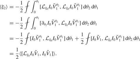 \begin{align} \langle \xi_2\rangle& = -\frac{1}{2}{\unicode{x2A0F}}\int_0^{\theta_1}[{\mathcal{L}}_{\xi_0} I_0 \tilde{V}_1^{\theta_2},{\mathcal{L}}_{\xi_0} I_0 \tilde{V}_1^{\theta_1}]\,\textrm{d}\theta_2\,\textrm{d}\theta_1\nonumber\\ & = -\frac{1}{2}{\unicode{x2A0F}}\int_0^{\theta_1}[\partial_{\theta_2} I_0 \tilde{V}_1^{\theta_2},{\mathcal{L}}_{\xi_0} I_0 \tilde{V}_1^{\theta_1}]\,\textrm{d}\theta_2\,\textrm{d}\theta_1\nonumber\\ & = -\frac{1}{2}{\unicode{x2A0F}}[ I_0 \tilde{V}_1^{\theta_1},{\mathcal{L}}_{\xi_0} I_0 \tilde{V}_1^{\theta_1}]\,\textrm{d}\theta_1+ \frac{1}{2}{\unicode{x2A0F}}[ I_0 \tilde{V}_1,{\mathcal{L}}_{\xi_0} I_0 \tilde{V}_1^{\theta_1}]\,\textrm{d}\theta_2\,\textrm{d}\theta_1\nonumber\\ & = \frac{1}{2} \langle [ {\mathcal{L}}_{\xi_0} I_0 \tilde{V}_1,I_0 \tilde{V}_1] \rangle. \end{align}
Next observe that condition (2.35) is equivalent to the linear equation
 \begin{align} {\mathcal{L}}_{V_0}\tilde{\xi}_2 &= [\xi_0,V_2] + [\xi_1,V_1]^{\textrm{osc}}\nonumber\\ & = {\mathcal{L}}_{\xi_0} \tilde{V}_2 + {\mathcal{L}}_{\xi_0} [ I_0\tilde{V}_1, \langle V_1\rangle] + [{\mathcal{L}}_{\xi_0} I_0 \tilde{V}_1,\tilde{V}_1]^{\textrm{osc}}, \end{align}
which has the unique solution
 \begin{align} \tilde{\xi}_2 & = {\mathcal{L}}_{\xi_0}(I_0\tilde{V}_2 + I_0[ I_0\tilde{V}_1, \langle V_1\rangle]) + I_0 [{\mathcal{L}}_{\xi_0} I_0 \tilde{V}_1,\tilde{V}_1]^{\textrm{osc}}\nonumber\\ & = {\mathcal{L}}_{\xi_0}\left(I_0\tilde{V}_2 + I_0[ I_0\tilde{V}_1, \langle V_1\rangle] + \frac{1}{2}I_0[I_0\tilde{V}_1,\tilde{V}_1]^{\textrm{osc}}\right) + \frac{1}{2}[{\mathcal{L}}_{\xi_0} I_0\tilde{V}_1, I_0\tilde{V}_1]^{\textrm{osc}}. \end{align}
On the second line of (2.39) we have used the identity
 \begin{equation} I_0[{\mathcal{L}}_{\xi_0} I_0\tilde{V}_1,\tilde{V}_1]^{\textrm{osc}} = \frac{1}{2}[{\mathcal{L}}_{\xi_0} I_0\tilde{V}_1,I_0\tilde{V}_1]^{\textrm{osc}} + \frac{1}{2}{\mathcal{L}}_{\xi_0} I_0[ I_0\tilde{V}_1, \tilde{V}_1]^{\textrm{osc}},\end{equation}
which follows from the non-trivial recursive relationship
 \begin{align} I_0[{\mathcal{L}}_{\xi_0} I_0\tilde{V}_1,\tilde{V}_1]^{\textrm{osc}} &=I_0[{\mathcal{L}}_{\xi_0} I_0\tilde{V}_1,{\mathcal{L}}_{V_0}I_0\tilde{V}_1]^{\textrm{osc}}\nonumber\\ & = [{\mathcal{L}}_{\xi_0} I_0\tilde{V}_1,I_0\tilde{V}_1]^{\textrm{osc}} - I_0[{\mathcal{L}}_{\xi_0} \tilde{V}_1,I_0\tilde{V}_1]^{\textrm{osc}}\nonumber\\ & = [{\mathcal{L}}_{\xi_0} I_0\tilde{V}_1,I_0\tilde{V}_1]^{\textrm{osc}} + {\mathcal{L}}_{\xi_0} I_0[ I_0\tilde{V}_1, \tilde{V}_1]^{\textrm{osc}} - I_0[{\mathcal{L}}_{\xi_0} I_0\tilde{V}_1, \tilde{V}_1]^{\textrm{osc}}. \end{align}
Adding (2.37) and (2.39) demonstrates the first part of our claim, in addition to giving the desired formula (2.25) for  $\xi _2$. As for the second part of our claim, the expression (2.37) for
  $\langle \xi _2\rangle$ implies
 \begin{align} \langle [\xi_1,V_1]\rangle + \langle [\xi_2,V_0] \rangle & = \langle [ {\mathcal{L}}_{\xi_0} I_0\tilde{V}_1,\tilde{V}_1]\rangle+ \langle [\langle\xi_2\rangle,V_0] \rangle\nonumber\\ & = \langle [ {\mathcal{L}}_{\xi_0} I_0\tilde{V}_1,\tilde{V}_1]\rangle + \frac{1}{2}\langle [[{\mathcal{L}}_{\xi_0} I_0\tilde{V}_1, I_0\tilde{V}_1],V_0] \rangle\nonumber\\ & = \langle [ {\mathcal{L}}_{\xi_0} I_0\tilde{V}_1,\tilde{V}_1]\rangle -\frac{1}{2}\langle [{\mathcal{L}}_{\xi_0} \tilde{V}_1, I_0\tilde{V}_1] \rangle - \frac{1}{2}\langle [{\mathcal{L}}_{\xi_0} I_0\tilde{V}_1, \tilde{V}_1] \rangle \nonumber\\ & = 0, \end{align}
as claimed.
The pattern established at the previous orders in  $\epsilon$ continues with the
  $O(\epsilon ^3)$ coefficients of
  $Z_\epsilon$ and
  $[\xi _\epsilon , V_\epsilon ]$. Vanishing of the third-order coefficients is equivalent to the trio of conditions
 \begin{gather} \langle \xi_3\rangle = -\frac{1}{2}{\unicode{x2A0F}} \int_0^{\theta_1} [\xi_1^{\theta_2},\xi_2^{\theta_1}]\,\textrm{d}\theta_2\,\textrm{d}\theta_1-\frac{1}{2}{\unicode{x2A0F}} \int_0^{\theta_1} [\xi_2^{\theta_2},\xi_1^{\theta_1}]\,\textrm{d}\theta_2\,\textrm{d}\theta_1\nonumber\\ \hspace{80pt} - \frac{1}{6}{\unicode{x2A0F}} \int_0^{\theta_1}\int_0^{\theta_2} ([\xi_1^{\theta_3},[\xi_1^{\theta_2},\xi_1^{\theta_1}]] +[[\xi_1^{\theta_3},\xi_1^{\theta_2}],\xi_1^{\theta_1}])\,\textrm{d}\theta_3\,\textrm{d}\theta_2\,\textrm{d}\theta_1, \end{gather}
 \begin{gather}0 = [\xi_0,\tilde{V}_3] + [\xi_1,V_2]^{\textrm{osc}} + [\xi_2,V_1]^{\textrm{osc}} + [\xi_3,V_0], \end{gather}
 \begin{gather}0 = \langle [\xi_1,V_2]\rangle + \langle [\xi_2,V_1]\rangle + [\langle \xi_3\rangle ,V_0]. \end{gather}
To see that (2.43) determines  $\langle \xi _3\rangle$ first use Fubini's theorem and the Lie derivative formula to simplify the double integrals as
 \begin{align} \langle \xi_3\rangle & = \langle [\tilde{\xi}_2,I_0\tilde{V}_1]\rangle + [I_0\tilde{V}_1,\langle \xi_2\rangle]\nonumber\\ &\quad - \frac{1}{6}{\unicode{x2A0F}} \int_0^{\theta_1}\int_0^{\theta_2} ([\xi_1^{\theta_3},[\xi_1^{\theta_2},\xi_1^{\theta_1}]]+[[\xi_1^{\theta_3},\xi_1^{\theta_2}],\xi_1^{\theta_1}]\bigg)\,\textrm{d}\theta_3\,\textrm{d}\theta_2\,\textrm{d}\theta_1. \end{align}
Next use the same techniques to perform the  $\theta _3$ and
  $\theta _1$ integrations in the triple integral according to
 \begin{align} \langle \xi_3\rangle & = \langle [\tilde{\xi}_2,I_0\tilde{V}_1]\rangle + [I_0\tilde{V}_1,\langle \xi_2\rangle]\nonumber\\ & = \langle [\tilde{\xi}_2,I_0\tilde{V}_1]\rangle + [I_0\tilde{V}_1,\langle \xi_2\rangle]- \frac{1}{3}\langle[[{\mathcal{L}}_{\xi_0} I_0\tilde{V}_1,I_0\tilde{V}_1],I_0\tilde{V}_1] \rangle \nonumber\\ &\quad - \frac{1}{3}{\unicode{x2A0F}} \int_0^{\theta_1} ([I_0\tilde{V}_1^{\theta_2},[\xi_1^{\theta_2},I_0\tilde{V}_1]] +[[I_0\tilde{V}_1^{\theta_2},\xi_1^{\theta_2}],I_0\tilde{V}_1])\,\textrm{d}\theta_3\,\textrm{d}\theta_2. \end{align}
Finally apply the identity
 \begin{equation} [I_0\tilde{V}_1^{\theta_2},[\xi_1^{\theta_2},I_0\tilde{V}_1]] = \frac{1}{2}\partial_{\theta_2} [I_0\tilde{V}_1^{\theta_2},[I_0\tilde{V}_1^{\theta_2},I_0\tilde{V}_1]] -\frac{1}{2}[[{\mathcal{L}}_{\xi_0} I_0\tilde{V}_1^{\theta_2},I_0\tilde{V}_1^{\theta_2}],I_0\tilde{V}_1] \end{equation}
to obtain
 \begin{align} \langle \xi_3\rangle & = \langle [\tilde{\xi}_2,I_0\tilde{V}_1]\rangle + [I_0\tilde{V}_1,\langle \xi_2\rangle]- \frac{1}{3}\langle[[{\mathcal{L}}_{\xi_0} I_0\tilde{V}_1,I_0\tilde{V}_1],I_0\tilde{V}_1] \rangle \nonumber\\ &\quad + \frac{1}{2} [\langle[{\mathcal{L}}_{\xi_0} I_0\tilde{V}_1,I_0\tilde{V}_1]\rangle,I_0\tilde{V}_1]\nonumber\\ & = \langle [\tilde{\xi}_2,I_0\tilde{V}_1]\rangle - \frac{1}{3}\langle[[{\mathcal{L}}_{\xi_0} I_0\tilde{V}_1,I_0\tilde{V}_1],I_0\tilde{V}_1] \rangle\nonumber\\ & = \langle [{\mathcal{L}}_{\xi_0} I_0\tilde{V}_2,I_0\tilde{V}_1]\rangle + \langle [{\mathcal{L}}_{\xi_0} I_0[I_0\tilde{V}_1,\langle V_1\rangle],I_0\tilde{V}_1] \rangle \nonumber\\ &\quad + \frac{1}{2}\langle [{\mathcal{L}}_{\xi_0} I_0[I_0\tilde{V}_1,\tilde{V}_1]^{\textrm{osc}},I_0\tilde{V}_1] \rangle + \frac{1}{6} \langle[[{\mathcal{L}}_{\xi_0} I_0\tilde{V}_1,I_0\tilde{V}_1],I_0\tilde{V}_1]\rangle. \end{align}
For the oscillating part of  $\xi _3$ use (2.44) to obtain the general formula
 \begin{equation} \tilde{\xi}_3 = I_0[\xi_0,\tilde{V}_3] + I_0[\xi_1,V_2]^{\textrm{osc}} + I_0[\xi_2,V_1]^{\textrm{osc}}.\end{equation}
Using (2.24) for  $\xi _1$ and (2.25) for
  $\xi _2$ this formula for
  $\tilde {\xi }_3$ may be added to (2.49) and then manipulated so as to yield (2.26). The details of this tedious calculation may be found in appendix B. The proof will now be complete as soon as we show that if
  $\xi _1,\ \xi _2$, and
  $\xi _3$ are given by (2.24)–(2.26), respectively, then condition (2.45) is satisfied automatically. This may be seen by the following direct calculation with
  $I = \langle [\xi _1,V_2]\rangle + \langle [\xi _2,V_1]\rangle + [\langle \xi _3\rangle ,V_0]$,
 \begin{align} I & = \langle[{\mathcal{L}}_{\xi_0}I_0\tilde{V}_1,\tilde{V}_2] \rangle\nonumber\\ &\quad + \langle [ {\mathcal{L}}_{\xi_0} I_0\tilde{V}_2 + {\mathcal{L}}_{\xi_0} I_0[ I_0\tilde{V}_1, \langle V_1\rangle] + \frac{1}{2}{\mathcal{L}}_{\xi_0} I_0[I_0\tilde{V}_1,\tilde{V}_1]^{\textrm{osc}} + \frac{1}{2}[{\mathcal{L}}_{\xi_0} I_0\tilde{V}_1, I_0\tilde{V}_1],V_1] \rangle \nonumber\\ &\quad -{\mathcal{L}}_{V_0}(\langle [{\mathcal{L}}_{\xi_0} I_0\tilde{V}_2,I_0\tilde{V}_1]\rangle + \langle [{\mathcal{L}}_{\xi_0} I_0[I_0\tilde{V}_1,\langle V_1\rangle],I_0\tilde{V}_1]\rangle)\nonumber\\ &\quad -{\mathcal{L}}_{V_0}\left(\frac{1}{2}\langle [{\mathcal{L}}_{\xi_0} I_0[I_0\tilde{V}_1,\tilde{V}_1]^{\textrm{osc}},I_0\tilde{V}_1] \rangle + \frac{1}{6} \langle[[{\mathcal{L}}_{\xi_0} I_0\tilde{V}_1,I_0\tilde{V}_1],I_0\tilde{V}_1]\rangle\right)\nonumber\\ & = \langle [{\mathcal{L}}_{\xi_0}I_0\tilde{V}_1,\tilde{V}_2]\rangle + \frac{1}{2}\langle[[{\mathcal{L}}_{\xi_0}I_0\tilde{V}_1,I_0\tilde{V}_1],\langle V_1\rangle] \rangle + \frac{1}{2}\langle [[{\mathcal{L}}_{\xi_0}I_0\tilde{V}_1,I_0\tilde{V}_1],\tilde{V}_1]\rangle\nonumber\\ &\quad - \frac{1}{6}\langle [[{\mathcal{L}}_{\xi_0}\tilde{V}_1,I_0\tilde{V}_1],I_0\tilde{V}_1]\rangle-\frac{1}{6}\langle [[{\mathcal{L}}_{\xi_0}I_0\tilde{V}_1,\tilde{V}_1],I_0\tilde{V}_1] \rangle-\frac{1}{6}\langle [[{\mathcal{L}}_{\xi_0}I_0\tilde{V}_1,I_0\tilde{V}_1],\tilde{V}_1] \rangle\nonumber\\ &\quad+\left\langle \left[\left(\tilde{V}_2 + [I_0\tilde{V}_1,\langle V_1\rangle] + \frac{1}{2}[I_0\tilde{V}_1,\tilde{V}_1]^{\textrm{osc}}\right),{\mathcal{L}}_{\xi_0}I_0\tilde{V}_1\right]\right\rangle\nonumber\\ & = \frac{1}{3}\langle [[{\mathcal{L}}_{\xi_0}I_0\tilde{V}_1,I_0\tilde{V}_1],\tilde{V}_1]\rangle- \frac{1}{6}\langle [[{\mathcal{L}}_{\xi_0}\tilde{V}_1,I_0\tilde{V}_1],I_0\tilde{V}_1]\rangle-\frac{1}{6}\langle [[{\mathcal{L}}_{\xi_0}I_0\tilde{V}_1,\tilde{V}_1],I_0\tilde{V}_1] \rangle\nonumber\\ &\quad+\frac{1}{2}\left\langle \left[[I_0\tilde{V}_1,\tilde{V}_1]^{\textrm{osc}},{\mathcal{L}}_{\xi_0}I_0\tilde{V}_1\right]\right\rangle\nonumber\\ &=\frac{1}{3}\langle [[{\mathcal{L}}_{\xi_0}I_0\tilde{V}_1,I_0\tilde{V}_1],\tilde{V}_1]\rangle - \frac{1}{3}\langle [[\tilde{V}_1,I_0\tilde{V}_1],{\mathcal{L}}_{\xi_0}I_0\tilde{V}_1]\rangle+\frac{1}{3}\langle [[\tilde{V}_1,{\mathcal{L}}_{\xi_0}I_0\tilde{V}_1],I_0\tilde{V}_1]\rangle\nonumber\\ &= 0. \end{align}
3. Noether's theorem and adiabatic invariants
In the previous section we explained that all nearly periodic systems admit a roto-rate vector. In this sense every nearly periodic system has an approximate  $U(1)$ symmetry. In this subsection we will show that if a nearly periodic system happens to have a Hamiltonian structure as well then there is an approximate conserved quantity
  $\mu _\epsilon = \mu _0 + \epsilon \mu _1 + \epsilon ^2\mu _2 + \cdots$ associated with its approximate
  $U(1)$ symmetry. In effect we will prove an asymptotic version of Noether's theorem that applies to Hamiltonian nearly periodic systems. We will work in the setting of presymplectic Hamiltonian systems with
  $\epsilon$-dependent exact presymplectic structures. In the setting of
  $\epsilon$-independent exact symplectic Hamiltonian systems Kruskal (Reference Kruskal1962) gave an abstract proof of an analogous result, in the sense that formulas were not provided for the approximate conserved quantity. Here, we will improve Kruskal's results by providing (the first several terms of) the missing formulas, and by allowing for a much broader class of nearly periodic Hamiltonian systems. In particular we will provide formulas for
  $\mu _0,\mu _1,\mu _2,$ and
  $\mu _3$. For a discussion of some of the subtleties associated with adiabatic invariants for nearly periodic Poisson systems, see Omohundro (Reference Omohundro1986).
Before discussing the asymptotic version of Noether's theorem it is useful to discuss the usual Noether's theorem in a coordinate-independent manner. We will focus our attention on Noether's theorem for Hamiltonian systems on presymplectic manifolds that admit a  $U(1)$ symmetry.
To that end, suppose  $X$ is a vector field on a manifold
  $Z$ and assume that there is a
  $1$-form
  $\vartheta$ and a smooth function
  $H$ such that
  $\iota _X\mathbf{d}\vartheta = -\mathbf{d}H$. The dynamical system defined by
  $X$ is then known as a (presymplectic) Hamiltonian system, the
  $2$-form
  $\omega = -\mathbf{d}\vartheta$ is called the presymplectic form and the scalar
  $H$ is called the Hamiltonian. Noether's theorem applies to such systems. In particular if
  $\varPhi _\theta :Z\rightarrow Z$ is a
  $U(1)$-action (
 $\theta \in U(1) = \mathbb {R}/2{\rm \pi}$) on
  $Z$ that leaves the Hamiltonian invariant,
  $\varPhi _\theta ^*H = H$, and that leaves the presymplectic form invariant,
  $\varPhi _\theta ^*\omega = \omega$, then the scalar
  $\mu = \iota _\xi \langle \vartheta \rangle$ is a constant of motion for
  $X$. Here,
  $\xi = \partial _\theta \varPhi _\theta \mid _{\theta =0}$ is the infinitesimal generator for the
  $U(1)$-action and
  $\langle \vartheta \rangle = (2{\rm \pi} )^{-1}\int _0^{2{\rm \pi} }\varPhi _\theta ^*\vartheta \,\textrm {d}\theta$. The scalar
  $\mu$ is the Noether-invariant associated with the
  $U(1)$-action
  $\varPhi _\theta$. The proof that
  $\mu$ is a conserved quantity for
  $X$ follows from the following simple calculation:
  ${\mathcal {L}}_{X}\mu = \iota _X\mathbf{d}\iota _\xi \langle \vartheta \rangle = \iota _X{\mathcal {L}}_{\xi }\langle \vartheta \rangle - \iota _X\iota _\xi \mathbf{d}\langle \vartheta \rangle = \iota _X{\mathcal {L}}_{\xi }\langle \vartheta \rangle - {\mathcal {L}}_\xi H = 0$.
Now suppose that  $\dot {z} = \epsilon ^{-1}V_\epsilon (z)$ defines a nearly periodic system that happens to be Hamiltonian. Concretely this means the following.
Definition 3.1 (Nearly periodic Hamiltonian system) A nearly periodic system  $\dot {z} = \epsilon ^{-1}V_\epsilon (z)$ is a nearly periodic Hamiltonian system if there is some
  $1$-form
  $\vartheta _\epsilon$ and some function
  $H_\epsilon$ such that
  $\iota _{V_\epsilon }\mathbf{d}\vartheta _\epsilon = -\mathbf{d}H_\epsilon$.
  $H_\epsilon$ and
  $\vartheta _\epsilon$ are required to depend smoothly on
  $\epsilon$ in a neighbourhood of
  $\epsilon = 0$.
By mimicking the key parts of the  $U(1)$ Noether theorem from the previous paragraph we will now prove that there exists a formal power series
  $\mu _\epsilon = \mu _0 + \epsilon \mu _1 + \cdots$ that is constant along integral curves of
  $V_\epsilon$ to all-orders in
  $\epsilon$. In other words
  ${\mathcal {L}}_{V_\epsilon }\mu _\epsilon = 0$ in the sense of formal power series. The proof will be consistent with this article's goal of avoiding the well-known coordinate transform-based methods.
Before giving the proof it is useful to first give a variant of a technical Lemma originally proved in Kruskal (Reference Kruskal1962). (Kruskal refers to his ‘Theorem of Phase Independence’ in Section C.1.)
Lemma 3.2 (Bootstrapping of  $U(1)$ averages)
Fix a nearly periodic system  $\dot {z} = \epsilon ^{-1}V_\epsilon (x)$. Suppose that
  $\tau _\epsilon$ is any differential form on
  $Z$ that depends smoothly on
  $\epsilon$. If
  $\tau _\epsilon$ is constant along the flow of
  $V_\epsilon$, i.e.
  ${\mathcal {L}}_{V_\epsilon }\tau _\epsilon =0$, and is almost
  $U(1)$-invariant in the sense that
  ${\mathcal {L}}_{\xi _0}\tau _0=0$, then in fact
  $\tau _\epsilon$ satisfies
  ${\mathcal {L}}_{\xi _\epsilon }\tau _\epsilon = 0$ to all orders in
  $\epsilon$.
Proof. As mentioned earlier in the proof of Theorem 2.7, Kruskal (Reference Kruskal1962) shows that there is a formal near-identity diffeomorphism  $T_\epsilon :Z\rightarrow Z$ such that
  $T_{\epsilon *}\xi _\epsilon = \xi _0$. (In fact there are many such
  $T_\epsilon$.) Set
  $V_\epsilon ^* = T_{\epsilon *}V_\epsilon$ and
  $\tau _\epsilon ^* = T_{\epsilon *}\tau _\epsilon$.
Since  $\tau _\epsilon$ is constant along the
  $V_\epsilon$-flow it is also true that
  $\tau _\epsilon ^*$ is constant along the
  $V_\epsilon ^*$-flow, i.e.
  ${\mathcal {L}}_{V_\epsilon ^*}\tau _\epsilon ^*=0$. In light of the fact that
  $[\xi _0,V_\epsilon ^*] = T_{\epsilon *}[\xi _\epsilon ,V_\epsilon ] = 0$ this implies
  ${\mathcal {L}}_{V_\epsilon ^*}{\mathcal {L}}_{\xi _0}\tau _\epsilon ^*=0$. The
  $O(1)$ coefficient of this formal power series identity is
  ${\mathcal {L}}_{V_0}{\mathcal {L}}_{\xi _0}\tau _0 = 0$, which is trivially satisfied because
  $\tau _\epsilon$ is nearly
  $U(1)$-invariant by hypothesis. On the other hand, the
  $O(\epsilon )$ coefficient is
  ${\mathcal {L}}_{V_0}{\mathcal {L}}_{\xi _0}\tau _1^* = 0$, which says that
  ${\mathcal {L}}_{\xi _0}\tau _1^*$ is constant along the
  $V_0$-flow. We claim that this can only be true if
  ${\mathcal {L}}_{\xi _0}\tau _1^*=0$. To see this set
  $\tilde {\alpha } ={\mathcal {L}}_{\xi _0}\tau _1^*$. The Lie derivative of
  $\tilde {\alpha }$ along
  $V_0$ is given by
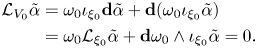 \begin{align} {\mathcal{L}}_{V_0}\tilde{\alpha} &= \omega_0\iota_{\xi_0}\mathbf{d}\tilde{\alpha} + \mathbf{d}(\omega_0\iota_{\xi_0}\tilde{\alpha})\nonumber\\ & = \omega_0{\mathcal{L}}_{\xi_0}\tilde{\alpha} + \mathbf{d}\omega_0\wedge \iota_{\xi_0}\tilde{\alpha} = 0. \end{align}
Contracting this formula with  $\xi _0$ therefore implies
  $\omega _0 {\mathcal {L}}_{\xi _0}\iota _{\xi _0}\tilde {\alpha } =0$. Because the
  $U(1)$-average of
  $\tilde {\alpha }$ is zero and
  $\omega _0$ is nowhere vanishing this requires
  $\iota _{\xi _0}\tilde {\alpha }=0$. But by (3.1) this implies
  $\omega _0{\mathcal {L}}_{\xi _0}\tilde {\alpha } = 0$, which can only be satisfied if
  $\tilde {\alpha }=0$, as desired. This shows, in particular, that
  ${\mathcal {L}}_{\xi _0}\tau _\epsilon ^* = O(\epsilon ^2)$.
To complete the proof we will now show that if, for some integer  $n\geq 2$,
  ${\mathcal {L}}_{\xi _0}\tau _\epsilon ^* = O(\epsilon ^n)$ then in fact
  ${\mathcal {L}}_{\xi _0}\tau _\epsilon ^* = O(\epsilon ^{n+1})$. If this is true then, by induction,
  ${\mathcal {L}}_{\xi _0}\tau _\epsilon ^* =0$ as a formal power series, which would imply the desired result since
  $T_\epsilon ^*({\mathcal {L}}_{\xi _0}\tau _\epsilon ^*) = {\mathcal {L}}_{\xi _\epsilon }\tau _\epsilon$. Because
  ${\mathcal {L}}_{\xi _0}\tau _\epsilon ^* = O(\epsilon ^n)$ the differential forms
  ${\mathcal {L}}_{\xi _0}\tau _k^*$ for
  $k\in \{0,1,\dots , n-1\}$ must each vanish. Therefore
  ${\mathcal {L}}_{\xi _0}\tau _\epsilon ^*=\epsilon ^{n}\,{\mathcal {L}}_{\xi _0}\tau _n^* + O(\epsilon ^{n+1})$. But since
  ${\mathcal {L}}_{V_\epsilon ^*}{\mathcal {L}}_{\xi _0}\tau _\epsilon ^* = 0$ to all orders in
  $\epsilon$ this means
  ${\mathcal {L}}_{V_0}{\mathcal {L}}_{\xi _0}\tau _n^* = 0$. Repeating the argument from the previous paragraph with
  $\tilde {\alpha } = {\mathcal {L}}_{\xi _0}\tau _n^*$ then shows that in fact
  ${\mathcal {L}}_{\xi _0}\tau _n^*=0$. Therefore
  ${\mathcal {L}}_{\xi _0}\tau _\epsilon ^*=\epsilon ^{n} {\mathcal {L}}_{\xi _0}\tau _n^* + O(\epsilon ^{n+1}) = O(\epsilon ^{n+1})$, as claimed.
Next we will show that the limiting roto-rate vector  $\xi _0$ associated with a nearly periodic Hamiltonian system is itself Hamiltonian.
Lemma 3.3 (Hamiltonian structure of the limiting roto-rate) If  $\dot {z} = \epsilon ^{-1}V_\epsilon (z)$ is a nearly periodic Hamiltonian system with frequency function
  $\omega _0$, limiting roto-rate
  $\xi _0$, presymplectic form
  $-\mathbf{d}\vartheta _\epsilon$, and Hamiltonian
  $H_\epsilon$ then there exists a function
  $\mu _0:Z\rightarrow \mathbb {R}$ such that
  $\omega _0^{-1}\mathbf{d}H_0 = \mathbf{d}\mu _0$. In particular, the limiting roto-rate
  $\xi _0$ satisfies
  $\iota _{\xi _0}\mathbf{d}\vartheta _0 = -\mathbf{d}\mu _0$, and is therefore Hamiltonian with presymplectic form
  $-\mathbf{d}\vartheta _0$ and Hamiltonian
  $\mu _0$.
Proof. Because  $\iota _{V_\epsilon }\mathbf{d}\vartheta _\epsilon = -\mathbf{d}H_\epsilon$ and everything depends smoothly on
  $\epsilon$ it must also be true that
  $\omega _0\iota _{\xi _0}\mathbf{d}\vartheta _0 = -\mathbf{d}H_0$. Contracting both sides of this identity with
  $\xi _0$ implies
  ${\mathcal {L}}_{\xi _0}H_0 = 0$. Pulling back the identity along
  $\exp (\theta \,\xi _0)$ and then averaging over
  $\theta$ therefore implies
  $\omega _0\iota _{\xi _0}\mathbf{d}\langle \vartheta _0\rangle =-\mathbf{d}H_0$. It follows that the function
  $\mu _0 = \iota _{\xi _0}\langle \vartheta _0 \rangle$ satisfies
 \begin{equation} \mathbf{d}\mu_0 = \mathbf{d} \iota_{\xi_0}\langle\vartheta_0 \rangle = -\iota_{\xi_0}\mathbf{d}\langle \vartheta_0\rangle = \omega_0^{-1}\mathbf{d}H_0. \end{equation}
Finally we will prove the existence of an adiabatic invariant for any nearly periodic Hamiltonian system.
Theorem 3.4 (Existence of the adiabatic invariant) Let  $\dot {z} = \epsilon ^{-1}V_\epsilon (z)$ be a Hamiltonian nearly periodic system with presymplectic form
  $-\mathbf{d}\vartheta _\epsilon$ and Hamiltonian
  $H_\epsilon$. If
  $\xi _\epsilon$ denotes the associated roto-rate vector and
  $\bar {\vartheta }_\epsilon = (2{\rm \pi} )^{-1}\int _0^{2{\rm \pi} }\exp (\theta \,\xi _\epsilon )^*\vartheta _\epsilon \,\textrm {d}\theta$ denotes the formal
  $U(1)$ average of
  $\vartheta _\epsilon$ associated with
  $\xi _\epsilon$, then the formal power series
 \begin{equation} \mu_\epsilon = \iota_{\xi_\epsilon}\bar{\vartheta}_\epsilon \end{equation}
satisfies  ${\mathcal {L}}_{V_\epsilon }\mu _\epsilon = 0$.
Proof. First observe that the  $0$-form
  $H_\epsilon$ and the
  $2$-form
  $\mathbf{d}\vartheta _\epsilon$ are each constant along the flow
  $V_\epsilon$. Indeed,
  ${\mathcal {L}}_{V_\epsilon }H_\epsilon = \iota _{V_\epsilon }\mathbf{d}H_\epsilon =-\iota _{V_\epsilon }\iota _{V_\epsilon }\mathbf{d}\vartheta _\epsilon = 0$, and
  ${\mathcal {L}}_{V_\epsilon }\mathbf{d}\vartheta _\epsilon = \mathbf{d}\iota _{V_\epsilon }\mathbf{d}\vartheta _\epsilon = -\mathbf{d}\mathbf{d}H_\epsilon = 0$. (This is actually a general fact about presymplectic Hamiltonian systems.) Each of these forms is also nearly
  $U(1)$-invariant in the sense that
  ${\mathcal {L}}_{\xi _0}H_0 = 0$ and
  ${\mathcal {L}}_{\xi _0}\mathbf{d}\vartheta _0 = 0$. This can be seen by appealing to Lemma 3.3 and computing as follows:
 \begin{gather} {\mathcal{L}}_{\xi_0}H_0 = \iota_{\xi_0}\mathbf{d}H_0 = \iota_{\xi_0}\omega_0\mathbf{d}\mu_0 = - \omega_0\iota_{\xi_0}\iota_{\xi_0}\mathbf{d}\vartheta_\epsilon = 0, \end{gather}
 \begin{gather}{\mathcal{L}}_{\xi_0}\mathbf{d}\vartheta_0 = \mathbf{d}\iota_{\xi_0}\mathbf{d}\vartheta_0 = -\mathbf{d}\mathbf{d}\mu_0 = 0. \end{gather}
Therefore Lemma 3.2 implies
 \begin{gather} {\mathcal{L}}_{\xi_\epsilon}H_\epsilon = 0, \end{gather}
 \begin{gather}{\mathcal{L}}_{\xi_\epsilon}\mathbf{d}\vartheta_\epsilon = 0, \end{gather}
as formal power series.
It is now possible to directly compute  ${\mathcal {L}}_{V_\epsilon }\mu _\epsilon$ using the formula
 \begin{equation} {\mathcal{L}}_{V_\epsilon}\iota_{\xi_\epsilon}\bar{\vartheta}_\epsilon = \iota_{V_\epsilon}\mathbf{d}\iota_{\xi_\epsilon}\bar{\vartheta}_\epsilon =\iota_{V_\epsilon}{\mathcal{L}}_{\xi_\epsilon}\bar{\vartheta}_\epsilon + \iota_{\xi_\epsilon}\iota_{V_\epsilon}\mathbf{d}\bar{\vartheta}_\epsilon. \end{equation}
The first term on the right-hand side vanishes to all orders in  $\epsilon$ because
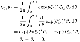 \begin{align} {\mathcal{L}}_{\xi_\epsilon}\bar{\vartheta}_\epsilon &= \frac{1}{2{\rm \pi}}\int_0^{2{\rm \pi}} \exp(\theta\xi_\epsilon)^*{\mathcal{L}}_{\xi_\epsilon}\vartheta_\epsilon\,\textrm{d}\theta\nonumber\\ & = \frac{1}{2{\rm \pi}}\int_0^{2{\rm \pi}} \frac{\textrm{d}}{\textrm{d}\theta} \exp(\theta \xi_\epsilon)^*\vartheta_\epsilon\,\textrm{d}\theta\nonumber\\ & = \exp(2{\rm \pi} \xi_\epsilon)^*\vartheta_\epsilon - \exp(0\,\xi_\epsilon)^*\vartheta_\epsilon\nonumber\\ &=\vartheta_\epsilon - \vartheta_\epsilon = 0. \end{align}
The second term on the right-hand side also vanishes to all orders because, by (3.7),
 \begin{equation} \mathbf{d}\bar{\vartheta}_\epsilon ={\unicode{x2A0F}} \exp(\theta\,\xi_\epsilon)^*\mathbf{d}\vartheta_\epsilon\,\textrm{d}\theta = \mathbf{d}\vartheta_\epsilon,\end{equation}
which implies
 \begin{equation} \iota_{\xi_\epsilon}\iota_{V_\epsilon}\mathbf{d}\bar{\vartheta}_\epsilon = \iota_{\xi_\epsilon}\iota_{V_\epsilon}\mathbf{d}{\vartheta}_\epsilon = -\iota_{\xi_\epsilon}\mathbf{d}H_\epsilon = -{\mathcal{L}}_{\xi_\epsilon}H_\epsilon =0, \end{equation}
by (3.6).
According to this Theorem the quantity  $\mu _\epsilon = \iota _{\xi _\epsilon }\bar {\vartheta }_\epsilon$ is an adiabatic invariant associated with any given nearly periodic Hamiltonian system. In fact
  $\mu _\epsilon$ is equivalent to the adiabatic invariant discussed in Kruskal (Reference Kruskal1962) when the presymplectic form
  $-\mathbf{d}\vartheta _\epsilon$ is globally equivalent to the canonical symplectic form
  $\mathbf{d}q^i\wedge \mathbf{d}p_i$. (Note that no degenerate presymplectic form is even locally equivalent to the canonical symplectic form.) Therefore the first four coefficients of the expansion
  $\mu _\epsilon = \mu _0 + \epsilon \mu _1 + \epsilon ^2\mu _2 + \cdots$, expressed in terms of
  $V_\epsilon$, comprise the main objective of this article. In principle the computation of these coefficients may be achieved using Theorem 2.11, which gives explicit formulas for
  $\xi _0,\xi _1,\xi _2,\xi _3$ in terms of
  $V_\epsilon$. Indeed, with knowledge of
  $\xi _\epsilon$ the one-form
  $\bar {\vartheta }_\epsilon$ may be computed directly by expanding
  $\exp (\theta \,\xi _\epsilon )$ in its formal power series in
  $\epsilon$. Once
  $\bar {\vartheta }_\epsilon$ has been computed
  $\mu _\epsilon$ can be obtained by merely forming the contraction
  $\iota _{\xi _\epsilon }\bar {\vartheta }_\epsilon$.
The following Theorem and its proof performs such a calculation and records the resulting formulas for  $\mu _0,\mu _1,\mu _2,\mu _3$. However, the proof does not proceed along the direct route of first computing
  $\bar {\vartheta }_\epsilon$. Instead it employs a method that reveals a striking feature of the series
  $\mu _\epsilon = \iota _{\xi _\epsilon }\bar {\vartheta }_\epsilon$: if
  $\vartheta _\epsilon$ is subject to the gauge transformation
  $\vartheta _\epsilon \mapsto \vartheta _\epsilon + \alpha _\epsilon = \vartheta ^\prime _\epsilon$, with
  $\alpha _\epsilon$ closed, then
  $\mu _\epsilon$ changes by at most a constant. This property may be seen abstractly using the following simple calculation,
 \begin{align} \mathbf{d}\iota_{\xi_\epsilon} \bar{\vartheta}_\epsilon^\prime & = \mathbf{d}{\unicode{x2A0F}}\iota_{\xi_\epsilon} \exp(\theta\,\xi_\epsilon)^*(\vartheta_\epsilon + \alpha_\epsilon)\,\textrm{d}\theta \nonumber\\ & = {\unicode{x2A0F}}\exp(\theta\,\xi_\epsilon)^*\mathbf{d}\iota_{\xi_\epsilon}(\vartheta_\epsilon + \alpha_\epsilon)\,\textrm{d}\theta\nonumber\\ & = {\unicode{x2A0F}} \exp(\theta\,\xi_\epsilon)^*{\mathcal{L}}_{\xi_\epsilon}(\vartheta_\epsilon + \alpha_\epsilon)\,\textrm{d}\theta - {\unicode{x2A0F}} \exp(\theta\,\xi_\epsilon)^*\iota_{\xi_\epsilon}\mathbf{d}(\vartheta_\epsilon + \alpha_\epsilon)\,\textrm{d}\theta \nonumber\\ & = {\unicode{x2A0F}} \frac{\textrm{d}}{\textrm{d}\theta}\exp(\theta\,\xi_\epsilon)^*(\vartheta_\epsilon + \alpha_\epsilon)\,\textrm{d}\theta - {\unicode{x2A0F}} \exp(\theta\,\xi_\epsilon)^*\iota_{\xi_\epsilon}\mathbf{d}\vartheta_\epsilon\,\textrm{d}\theta\nonumber\\ & = - {\unicode{x2A0F}} \exp(\theta \xi_\epsilon)^*\iota_{\xi_\epsilon}\mathbf{d}\vartheta_\epsilon\,\textrm{d}\theta, \end{align}
which shows that  $\mathbf{d}\mu _\epsilon$ is unchanged when
  $\vartheta _\epsilon$ is subject to a gauge transformation. In other words
  $\mathbf{d}\mu _\epsilon$ depends on
  $\vartheta _\epsilon$ only through the presymplectic form
  $-\mathbf{d}\vartheta _\epsilon$. The statement and proof of the following Theorem make this important property manifestly clear, order by order in
  $\epsilon$.
Theorem 3.5 (Formulas for the adiabatic invariant) Suppose  $\dot {z} = \epsilon ^{-1}V_\epsilon (z)$ is a nearly periodic Hamiltonian system with presymplectic form
  $-\mathbf{d}\vartheta _\epsilon$, Hamiltonian
  $H_\epsilon$ and limiting roto-rate vector
  $\xi _0$. The system's roto-rate vector
  $\xi _\epsilon$ is Hamiltonian in the sense that
 \begin{equation} \iota_{\xi_\epsilon}\mathbf{d}\vartheta_\epsilon = -\mathbf{d}\mu_\epsilon,\end{equation}
where  $\mu _\epsilon$ is the system's adiabatic invariant. Moreover, the first four coefficients of the series
  $\mu _\epsilon = \mu _0 + \epsilon \mu _1 + \epsilon ^2\mu _2 + \cdots$ are given by
 \begin{equation} \mu_0 =\iota_{\xi_0}\langle \vartheta_0\rangle, \end{equation}
 \begin{equation}\mu_1 = \iota_{\xi_0}\langle \vartheta_1\rangle - {\mathcal{L}}_{I_0\tilde{V}_1}\mu_0, \end{equation}
 \begin{equation}\mu_2 = \iota_{\xi_0}\langle \vartheta_2\rangle +\frac{1}{2}\left\langle \mathbf{d}\vartheta_0({\mathcal{L}}_{\xi_0}I_0\tilde{V}_1,I_0\tilde{V}_1)\right\rangle+ {\unicode{x2A0F}} \left( \frac{1}{2}{\mathcal{L}}_{Z_{1,\theta}}(\mu_1+\mu_1^\theta) +{\mathcal{L}}_{Z_{2,\theta}}\mu_0\right)\textrm{d}\theta, \end{equation}
 \begin{align} \mu_3& = \iota_{\xi_0}\langle \vartheta_3\rangle +\frac{2}{3}\langle \mathbf{d}\vartheta_2(I_0\tilde{V}_1,\xi_0)\rangle -\frac{2}{3}\langle\mathbf{d}\vartheta_2\rangle(I_0\tilde{V}_1,\xi_0) - \frac{1}{3}\langle \mathbf{d}\vartheta_1({\mathcal{L}}_{\xi_0}I_0\tilde{V}_1,I_0\tilde{V}_1)\rangle\nonumber\\ &\quad + \frac{1}{3}\left\langle \iota_{{\mathcal{L}}_{\xi_0}I_0\tilde{V}_1}\mathbf{d}\vartheta_1\right\rangle(I_0\tilde{V}_1) - \frac{1}{6}\langle \mathbf{d}\vartheta_0([{\mathcal{L}}_{\xi_0}I_0\tilde{V}_1,I_0\tilde{V}_1], I_0\tilde{V}_1)\rangle \nonumber\\ &\quad + \frac{1}{6}\mathbf{d}\vartheta_0(\langle [{\mathcal{L}}_{\xi_0}I_0\tilde{V}_1,I_0\tilde{V}_1]\rangle,I_0\tilde{V}_1) + \frac{1}{3}\langle \mathbf{d}\vartheta_0({\mathcal{L}}_{\xi_0}I_0\tilde{V}_1,I_0\tilde{V}_2)\rangle\nonumber\\ &\quad + \frac{1}{3}\langle \mathbf{d}\vartheta_0({\mathcal{L}}_{\xi_0}I_0\tilde{V}_1, I_0[I_0\tilde{V}_1,\langle V_1\rangle])\rangle+\frac{1}{6}\langle \mathbf{d}\vartheta_0({\mathcal{L}}_{\xi_0}I_0\tilde{V}_1,I_0[I_0\tilde{V}_1,\tilde{V}_1]^{\textrm{osc}})\rangle\nonumber\\ &\quad + \frac{1}{6}\langle \langle\mathbf{d}\vartheta_1 \rangle({\mathcal{L}}_{\xi_0}I_0\tilde{V}_1,I_0\tilde{V}_1)\rangle - \frac{1}{6}{\mathcal{L}}_{I_0\tilde{V}_1}\langle \mathbf{d}\vartheta_0({\mathcal{L}}_{\xi_0}I_0\tilde{V}_1,I_0\tilde{V}_1) \rangle\nonumber\\ &\quad +{\unicode{x2A0F}}\left(\frac{2}{3}{\mathcal{L}}_{Z_{2,\theta}}\mu_1 + \frac{1}{3}{\mathcal{L}}_{Z_{2,\theta}}\mu_1^\theta + \frac{1}{6}{\mathcal{L}}^2_{Z_{1,\theta}}\mu_1^\theta + \frac{1}{3}{\mathcal{L}}_{Z_{1,\theta}}\mu_2\right)\textrm{d}\theta\nonumber\\ &\quad + {\unicode{x2A0F}} {\mathcal{L}}_{Z_{3,\theta} + ({1}/{6})[Z_{1,\theta},Z_{2,\theta}]}\mu_0\,\textrm{d}\theta, \end{align}
where the vector fields  $Z_{1,\theta },Z_{2,\theta },Z_{3,\theta }$ are given by
 \begin{equation} Z_{1,\theta} = I_0\{\tilde{V}_1\}, \end{equation}
 \begin{equation}Z_{2,\theta} = I_0\{\tilde{V}_2\} + I_0[ I_0\{\tilde{V}_1\}, \langle V_1\rangle] + \frac{1}{2} I_0\{[I_0\tilde{V}_1,\tilde{V}_1]\}^{\textrm{osc}} - \frac{1}{2} [I_0\tilde{V}_1, I_0\tilde{V}_1^{\theta}], \end{equation}
 \begin{align} Z_{3,\theta} & = - \frac{1}{2}\int_0^\theta I_0[\langle [{\mathcal{L}}_{\xi_0} I_0\tilde{V}_1,I_0\tilde{V}_1]\rangle,\tilde{V}_1^{\theta_1}]\,\textrm{d}\theta_1\nonumber\\ &\quad +I_0\{\tilde{V}_3\} + I_0[ I_0\{\tilde{V}_1\},\langle V_2\rangle]^{\textrm{osc}} +I_0[ I_0\{\tilde{V}_2\},\langle V_1\rangle]^{\textrm{osc}}\nonumber\\ &\quad +\frac{1}{2} I_0\{[I_0\tilde{V}_2,\tilde{V}_1]\}^{\textrm{osc}}+ \frac{1}{2}I_0\{[I_0\tilde{V}_1,\tilde{V}_2]\}^{\textrm{osc}}+\frac{1}{3}I_0\{[I_0\tilde{V}_1,[I_0\tilde{V}_1,\tilde{V}_1]]\}^{\textrm{osc}}\nonumber\\ &\quad +I_0[ I_0[ I_0\{\tilde{V}_1\}, \langle V_1\rangle],\langle V_1\rangle] + \frac{1}{2}I_0[ I_0\{[I_0\tilde{V}_1,\tilde{V}_1]\}^{\textrm{osc}},\langle V_1\rangle]\nonumber\\ &\quad +\frac{1}{2}I_0\{[I_0\tilde{V}_1,[I_0\tilde{V}_1,\langle V_1\rangle]]\}^{\textrm{osc}}+ \frac{1}{12} [I_0(\tilde{V}_1^{\theta}+\tilde{V}_1),[I_0\tilde{V}_1,I_0\tilde{V}_1^{\theta}]]+\frac{1}{2}\{[I_0\tilde{V}_1,I_0\tilde{V}_2]\}\nonumber\\ &\quad +\frac{1}{2} \left[ I_0\{\tilde{V}_2\} + I_0[ I_0\{\tilde{V}_1\}, \langle V_1\rangle] + \frac{1}{2} I_0\{[I_0\tilde{V}_1,\tilde{V}_1]\}^{\textrm{osc}},I_0(\tilde{V}_1 + \tilde{V}_1^\theta)\right], \end{align}
where  $\{A\} = A^\theta - A$ for any vector field
  $A$.
$A$.
Proof. In order to establish (3.13) it is sufficient to compute the exterior derivative of  $\mu _\epsilon = \iota _{\xi _\epsilon }\bar {\vartheta }_\epsilon$ directly:
 \begin{equation} \mathbf{d}\mu_\epsilon = \mathbf{d}\iota_{\xi_\epsilon}\bar{\vartheta}_\epsilon = {\mathcal{L}}_{\xi_\epsilon}\bar{\vartheta}_\epsilon - \iota_{\xi_{\epsilon}}\mathbf{d}\bar{\vartheta}_\epsilon = -\iota_{\xi_{\epsilon}}\mathbf{d}\vartheta_\epsilon, \end{equation}
where we have made use of (3.9) and (3.10) from the proof of Lemma 3.4.
In order to obtain formulas for the  $\mu _k$ we will proceed in two steps. First we will use Stokes’ theorem to identify an alternative all-orders expression for
  $\mu _\epsilon$ that obviates how
  $\mu _\epsilon$ changes when
  $\vartheta _\epsilon$ is subject to the gauge transformation
  $\vartheta _\epsilon \mapsto \vartheta _\epsilon + \alpha _\epsilon$ with
  $\alpha _\epsilon$ closed. Then we will use the perturbative BCH formula (cf. Lemma 2.8) to expand the resulting expression as a power series in
  $\epsilon$.
Fix  $z\in Z$ and define the mapping
  $S:S^1\times [0,\epsilon ]\rightarrow Z:(\theta ,\lambda )\mapsto \exp (\theta \,\xi _{\lambda })(z)$. Choose an orientation for
  $S^1\times [0,\epsilon ]$ by declaring that the ordered basis
  $(\partial _\theta ,\partial _{\lambda })$ is positively oriented. By Stokes’ theorem
 \begin{equation} \int_{S^1\times[0,\epsilon]}\mathbf{d}S^*\vartheta_\epsilon = \int_{S^1\times\{0\}}S^*\vartheta_\epsilon - \int_{S^1\times\{\epsilon\}}S^*\vartheta_\epsilon,\end{equation}
where  $S^1\times \{0\}$ and
  $S^1\times \{\epsilon \}$ are each oriented in the sense of increasing
  $\theta \in S^1$. Accounting for these orientation conventions, (3.22) may be re-written in terms of definite integrals as
 \begin{align} \int_0^{\epsilon}\int_0^{2{\rm \pi}} [S^*\mathbf{d}\vartheta_\epsilon](\partial_\theta,\partial_{\lambda})\,\textrm{d}\theta\,\textrm{d}\lambda &= \int_0^{2{\rm \pi}} [\vartheta_\epsilon(\xi_0)](\exp(\theta\,\xi_0)(z)) \,\textrm{d}\theta\nonumber\\ &\quad -\int_0^{2{\rm \pi}} [\vartheta_\epsilon(\xi_\epsilon)](\exp(\theta\,\xi_\epsilon)(z))\,\textrm{d}\theta\nonumber\\ & = 2{\rm \pi} \iota_{\xi_0}\langle \vartheta_\epsilon\rangle(z) - 2{\rm \pi}\iota_{\xi_\epsilon}\bar{\vartheta}_\epsilon(z), \end{align}
which shows that the adiabatic invariant  $\mu _\epsilon = \iota _{\xi _\epsilon }\bar {\vartheta }_\epsilon$ may be expressed as
 \begin{equation} \mu_\epsilon(z) = \iota_{\xi_0}\langle \vartheta_\epsilon\rangle(z)+ {\unicode{x2A0F}} \int_0^{\epsilon}[S^*\mathbf{d}\vartheta_\epsilon](\partial_{\lambda},\partial_\theta)\,\textrm{d}\theta\,\textrm{d}\lambda.\end{equation}
Note that the second term on the right-hand side is in a somewhat unwieldy form. To rectify this issue first observe that the partial derivatives of  $\exp (\theta \xi _{\lambda })$ may be expressed as
 \begin{gather} \partial_\theta \exp(\theta\xi_{\lambda}) = \xi_{\lambda}\circ \exp(\theta\xi_{\lambda}), \end{gather}
 \begin{gather}\partial_{\lambda}\exp(\theta\xi_{\lambda}) = (\exp(-\theta\xi_0)^*\phi(-{\mathcal{L}}_{Z_{\lambda,\theta}}) \partial_{\lambda}Z_{\lambda,\theta})\circ \exp(\theta\,\xi_{\lambda}), \end{gather}
where  $Z_{\lambda ,\theta } = \ln (\exp (-\theta \xi _0)\circ \exp (\theta \xi _{\lambda }))$,
  $\phi (z) = (\exp (z) - 1)/z$, and we have made use of (2.11). Therefore the scalar
  $[S^*\mathbf{d}\vartheta _\epsilon ](\partial _{\lambda },\partial _\theta )$ may be written
 \begin{align} [S^*\mathbf{d}\vartheta_\epsilon](\partial_{\lambda},\partial_\theta) &=\exp(\theta\xi_{\lambda})^*(\mathbf{d}\vartheta_\epsilon(\exp(-\theta\,\xi_0)^*\phi(-{\mathcal{L}}_{Z_{\lambda,\theta}})\partial_{\lambda}Z_{\lambda,\theta},\xi_{\lambda}))(z)\nonumber\\ &=[\exp(Z_{\lambda,\theta})^*\mathbf{d}\vartheta_\epsilon^\theta](\exp(Z_{\lambda,\theta})^*\phi(-{\mathcal{L}}_{Z_{\lambda,\theta}})\partial_{\lambda}Z_{\lambda,\theta},\xi_{\lambda}) (z)\nonumber\\ &=[\exp(Z_{\lambda,\theta})^*\mathbf{d}\vartheta_\epsilon^\theta](\phi({\mathcal{L}}_{Z_{\lambda,\theta}})\partial_{\lambda}Z_{\lambda,\theta},\xi_{\lambda}) (z). \end{align}
An all-orders formula for the adiabatic invariant  $\mu _\epsilon$ is therefore
 \begin{equation} \mu_\epsilon = \iota_{\xi_0}\langle \vartheta_\epsilon\rangle + {\unicode{x2A0F}}\int_0^\epsilon [\exp(Z_{\lambda,\theta})^*\mathbf{d}\vartheta_\epsilon^\theta](\phi({\mathcal{L}}_{Z_{\lambda,\theta}})\partial_{\lambda}Z_{\lambda,\theta},\xi_{\lambda})\,\textrm{d}\lambda\,\textrm{d}\theta.\end{equation}
This is the formula we will use to compute the coefficients of the series  $\mu _\epsilon$. As promised, if
  $\vartheta _\epsilon$ is subject to the gauge transformation
  $\vartheta _\epsilon \mapsto \vartheta _\epsilon + \alpha _\epsilon$, with
  $\alpha _\epsilon$ closed, the formula (3.28) shows that
  $\mu _\epsilon$ transforms as
  $\mu _\epsilon \mapsto \mu _\epsilon + \iota _{\xi _0}\langle \alpha _\epsilon \rangle$. The change in
  $\mu _\epsilon$,
  $\Delta \mu _\epsilon = \iota _{\xi _0}\langle \alpha _\epsilon \rangle$, evaluated at
  $z\in Z$ may therefore be written as the closed loop integral
 \begin{equation} \Delta\mu_\epsilon(z) = \frac{1}{2{\rm \pi}}\oint_{\gamma_z} \alpha_\epsilon, \end{equation}
where the  $z$-dependent curve
  $\gamma _z$ is given by
  $\gamma _z(\theta ) = \exp (\theta \xi _0)(z)$. Because
  $\alpha _\epsilon$ is closed the integral
  $\oint _{\gamma _z}\alpha _\epsilon$ depends only on the homotopy class of
  $\gamma _z$. Since
  $\gamma _z$ depends continuously on
  $z$ this means
  $\Delta \mu _\epsilon$ is constant on path-connected components of
  $Z$. In particular, because the path-components are open subsets of
  $Z$,
$Z$,  $\mathbf{d}\Delta \mu _\epsilon = 0$, as inferred earlier from the abstract argument related to (3.12). In fact, this argument shows that the change in
  $\mu _\epsilon$ induced by a gauge transformation is equal to (
 $1/(2{\rm \pi} )$ times) the cohomology class of
  $\alpha _\epsilon$ paired with the cycle defined by the
  $\xi _0$-orbit
  $\gamma _z$. In particular if either (a) the first deRham cohomology group of
  $Z$ is trivial, or (b) the
  $\xi _0$-orbits are each homologous to a point then
  $\mu _\epsilon$ is gauge independent.
Expanding (3.28) in a power series is facilitated by first recording the more elementary power series expansions involving the coefficients of  $Z_{\lambda ,\theta } = \epsilon Z_{1,\theta } + \epsilon ^2Z_{2,\theta } + \epsilon ^3Z_{3,\theta } + \cdots$ given by
 \begin{gather} \exp(Z_{\lambda,\theta})^*\mathbf{d}\vartheta_\epsilon^\theta = \mathbf{d}\vartheta_\epsilon^\theta + \lambda {\mathcal{L}}_{Z_{1,\theta}}\mathbf{d}\vartheta_\epsilon^\theta +\lambda^2 \left({\mathcal{L}}_{Z_{2,\theta}} + \frac{1}{2}{\mathcal{L}}_{Z_{1,\theta}}^2\right)\mathbf{d}\vartheta_\epsilon^\theta+O(\lambda^3), \end{gather}
 \begin{gather}\phi({\mathcal{L}}_{Z_{\lambda,\theta}})\partial_\lambda Z_{\lambda,\theta} = Z_{1,\theta} + \lambda\,2Z_{2,\theta} + \lambda^2 \left(3 Z_{3,\theta} + \frac{1}{2}[Z_{1,\theta},Z_{2,\theta}]\right)+O(\lambda^3). \end{gather}
Substituting these expansions into (3.28) and performing the  $\lambda$-integrals then gives
 \begin{align} \mu_\epsilon & = \iota_{\xi_0}\langle\vartheta_\epsilon \rangle + \epsilon{\unicode{x2A0F}} \mathbf{d}\vartheta_\epsilon^\theta (Z_{1,\theta},\xi_0)\,\textrm{d}\theta \nonumber\\ &+ \epsilon^2{\unicode{x2A0F}}\left(\frac{1}{2}\left[{\mathcal{L}}_{Z_{1,\theta}}\mathbf{d}\vartheta_\epsilon^\theta\right] (Z_{1,\theta},\xi_0) + \frac{1}{2} \mathbf{d}\vartheta_\epsilon^\theta(Z_{1,\theta},\xi_1)+ \mathbf{d}\vartheta_\epsilon^\theta(Z_{2,\theta},\xi_0)\right)\,\textrm{d}\theta\nonumber\\ &\quad + \epsilon^3{\unicode{x2A0F}}\left(\frac{2}{3} \left[{\mathcal{L}}_{Z_{1,\theta}}\mathbf{d}\vartheta_\epsilon^\theta\right] (Z_{2,\theta},\xi_0) + \frac{2}{3} \mathbf{d}\vartheta_\epsilon^\theta (Z_{2,\theta},\xi_1) + \frac{1}{3} \left[{\mathcal{L}}_{Z_{1,\theta}}\mathbf{d}\vartheta_\epsilon^\theta\right](Z_{1,\theta},\xi_1)\right.\nonumber\\ &\quad+ \frac{1}{3}\left[{\mathcal{L}}_{Z_{2,\theta}}\mathbf{d}\vartheta_\epsilon^\theta + \frac{1}{2}{\mathcal{L}}_{Z_{1,\theta}}^2\mathbf{d}\vartheta_\epsilon^\theta\right](Z_{1,\theta},\xi_0) + \mathbf{d}\vartheta_\epsilon^\theta\left(Z_{3,\theta} + \frac{1}{6}[Z_{1,\theta},Z_{2,\theta}],\xi_0\right)\nonumber\\ & \quad \left.+ \frac{1}{3}\mathbf{d}\vartheta_\epsilon^\theta(Z_{1,\theta},\xi_2)\right)\,\textrm{d}\theta + O(\epsilon^4). \end{align}
The task of finding formulas for the  $\mu _k$ is therefore reduced to the problem of finding expressions for the
  $Z_{k,\theta }$ and then substituting them into (3.32).
In order to compute terms in the series  $Z_{\lambda ,\theta }$ it is helpful to reuse the perturbative BCH formula provided by Lemma 2.8. Setting
  $\epsilon = \lambda$,
  $A = \theta \xi _0$ and
  $B = \theta (\xi _1 + \lambda \,\xi _2 +\lambda ^2 \xi _3 + \cdots )$ the first several coefficients of
  $Z_{\lambda ,\theta }$ given by Lemma 2.8 may be expressed in integral form as
 \begin{gather} Z_{0,\theta} = 0, \end{gather}
 \begin{gather}Z_{1,\theta} = \int_0^\theta \xi_1^{\theta_1}\,\textrm{d}\theta_1, \end{gather}
 \begin{gather}Z_{2,\theta} =\int_0^\theta \xi_2^{\theta_1}\,\textrm{d}\theta_1+ \frac{1}{2}\int_0^\theta\int_0^{\theta_1}[\xi_1^{\theta_2},\xi_1^{\theta_1}]\,\textrm{d}\theta_2\,\textrm{d}\theta_1, \\ Z_{3,\theta} = \int_0^\theta \xi_3^{\theta_1}\,\textrm{d}\theta_1 + \frac{1}{2}\int_0^\theta\int_0^{\theta_1}[\xi_1^{\theta_2},\xi_2^{\theta_1}]\,\textrm{d}\theta_2\,\textrm{d}\theta_1+ \frac{1}{2}\int_0^\theta\int_0^{\theta_1}[\xi_2^{\theta_2},\xi_1^{\theta_1}]\,\textrm{d}\theta_2\,\textrm{d}\theta_1 \notag\end{gather}
 \begin{gather}+\frac{1}{6}\int_0^\theta\int_0^{\theta_1}\int_0^{\theta_2}\left([\xi_1^{\theta_3},[\xi_1^{\theta_2},\xi_1^{\theta_1}]] + [[\xi_1^{\theta_3},\xi_1^{\theta_2}],\xi_1^{\theta_1}]\right)\,\textrm{d}\theta_3\,\textrm{d}\theta_2\,\textrm{d}\theta_1. \end{gather}
Remarkably, most of the integrations indicated here may be carried out explicitly. First consider  $Z_{1,\theta }$. By inserting (2.24) for
  $\xi _1$ into (3.34) the vector field
  $Z_{1,\theta }$ may be expressed as
 \begin{align} Z_{1,\theta} &= \int_0^\theta {\mathcal{L}}_{\xi_0} I_0\tilde{V}_1^{\theta_1}\,\textrm{d}\theta_1\nonumber\\ &= I_0\tilde{V}_1^{\theta} - I_0\tilde{V}_1, \end{align}
which no longer contains any integrals. Similarly, by inserting (2.24) and (2.25) into (3.35) the vector field  $Z_{2,\theta }$ becomes
 \begin{align} Z_{2,\theta} & = \int_0^\theta \left( {\mathcal{L}}_{\xi_0} I_0\tilde{V}_2^{\theta_1} + {\mathcal{L}}_{\xi_0} I_0[ I_0\tilde{V}_1^{\theta_1}, \langle V_1\rangle] + \frac{1}{2}{\mathcal{L}}_{\xi_0} I_0[I_0\tilde{V}_1^{\theta_1},\tilde{V}_1^{\theta_1}]^{\textrm{osc}} \right)\,\textrm{d}\theta_1\nonumber\\ &\quad +\frac{1}{2} \int_0^\theta [{\mathcal{L}}_{\xi_0} I_0\tilde{V}_1^{\theta_1}, I_0\tilde{V}_1^{\theta_1}]\,\textrm{d}\theta_1 + \frac{1}{2}\int_0^\theta\int_0^{\theta_1}[{\mathcal{L}}_{\xi_0} I_0\tilde{V}_1^{\theta_2},{\mathcal{L}}_{\xi_0} I_0\tilde{V}_1^{\theta_1}]\,\textrm{d}\theta_2\,\textrm{d}\theta_1\nonumber\\ & = I_0\tilde{V}_2^{\theta} + I_0[ I_0\tilde{V}_1^{\theta}, \langle V_1\rangle] + \frac{1}{2} I_0[I_0\tilde{V}_1^{\theta},\tilde{V}_1^{\theta}]^{\textrm{osc}} \nonumber\\ &\quad -I_0\tilde{V}_2 - I_0[ I_0\tilde{V}_1, \langle V_1\rangle] - \frac{1}{2} I_0[I_0\tilde{V}_1,\tilde{V}_1]^{\textrm{osc}} +\frac{1}{2} \int_0^\theta [{\mathcal{L}}_{\xi_0} I_0\tilde{V}_1^{\theta_1}, I_0\tilde{V}_1^{\theta_1}]\,\textrm{d}\theta_1\nonumber\\ &\quad +\frac{1}{2}\int_0^\theta[I_0\tilde{V}_1^{\theta_1},{\mathcal{L}}_{\xi_0} I_0\tilde{V}_1^{\theta_1}]\,\textrm{d}\theta_1 - \frac{1}{2}\int_0^\theta [I_0\tilde{V}_1,{\mathcal{L}}_{\xi_0} I_0\tilde{V}_1^{\theta_1}]\,\textrm{d}\theta_1\nonumber\\ & = I_0\tilde{V}_2^{\theta} + I_0[ I_0\tilde{V}_1^{\theta}, \langle V_1\rangle] + \frac{1}{2} I_0[I_0\tilde{V}_1^{\theta},\tilde{V}_1^{\theta}]^{\textrm{osc}} \nonumber\\ &\quad -I_0\tilde{V}_2 - I_0[ I_0\tilde{V}_1, \langle V_1\rangle] - \frac{1}{2} I_0[I_0\tilde{V}_1,\tilde{V}_1]^{\textrm{osc}} - \frac{1}{2} [I_0\tilde{V}_1, I_0\tilde{V}_1^{\theta}], \end{align}
where the integrals that could not be evaluated by recognizing a total derivative have cancelled, apparently fortuitously. Finally consider  $Z_{3,\theta }$, which is the sum of a single integral, a pair of double integrals and a triple integral. The triple integral may be partially simplified by making use of (2.24) for
  $\xi _1$ and recognizing total derivatives according to
 \begin{align} &\frac{1}{6}\int_0^\theta\int_0^{\theta_1}\int_0^{\theta_2}([\xi_1^{\theta_3},[\xi_1^{\theta_2},\xi_1^{\theta_1}]] + [[\xi_1^{\theta_3},\xi_1^{\theta_2}],\xi_1^{\theta_1}])\,\textrm{d}\theta_3\,\textrm{d}\theta_2\,\textrm{d}\theta_1 \nonumber\\ &\quad =\frac{1}{3}\int_0^\theta[[{\mathcal{L}}_{\xi_0} I_0\tilde{V}_1^{\theta_2},I_0\tilde{V}_1^{\theta_2}],I_0\tilde{V}_1^{\theta_2}]\,\textrm{d}\theta_2\nonumber\\ &\qquad +\frac{1}{6}\int_0^\theta\left(\frac{1}{2}\partial_{\theta_2} [I_0\tilde{V}_1^{\theta_2},[I_0\tilde{V}_1^{\theta_2},I_0(\tilde{V}_1^{\theta} + \tilde{V}_1)]] - \frac{3}{2}[[{\mathcal{L}}_{\xi_0} I_0\tilde{V}_1^{\theta_2},I_0\tilde{V}_1^{\theta_2}],I_0(\tilde{V}_1^\theta + \tilde{V}_1)] \right)\textrm{d}\theta_2\nonumber\\ &\qquad +\frac{1}{6}[I_0\tilde{V}_1,[I_0\tilde{V}_1,I_0\tilde{V}_1^{\theta}]] - \frac{1}{6}[[I_0\tilde{V}_1,I_0\tilde{V}_1^\theta],I_0\tilde{V}_1^\theta] \nonumber\\ &\quad =\frac{1}{3}\int_0^\theta[[{\mathcal{L}}_{\xi_0} I_0\tilde{V}_1^{\theta_2},I_0\tilde{V}_1^{\theta_2}],I_0\tilde{V}_1^{\theta_2}]\,\textrm{d}\theta_2\nonumber\\ &\qquad -\frac{1}{4}\int_0^\theta[[{\mathcal{L}}_{\xi_0} I_0\tilde{V}_1^{\theta_2},I_0\tilde{V}_1^{\theta_2}],I_0(\tilde{V}_1^\theta + \tilde{V}_1)] \,\textrm{d}\theta_2\nonumber\\ &\qquad + \frac{1}{12} [I_0(\tilde{V}_1^{\theta}+\tilde{V}_1),[I_0\tilde{V}_1,I_0\tilde{V}_1^{\theta}]], \end{align}
where we have used the identity
 \begin{align} [I_0\tilde{V}_1^{\theta_2},[{\mathcal{L}}_{\xi_0} I_0\tilde{V}_1^{\theta_2},I_0(\tilde{V}_1^{\theta} + \tilde{V}_1)]]& =\frac{1}{2}\partial_{\theta_2}[I_0\tilde{V}_1^{\theta_2},[I_0\tilde{V}_1^{\theta_2},I_0(\tilde{V}_1^{\theta} + \tilde{V}_1)]]\nonumber\\ &\quad -\frac{1}{2}[[{\mathcal{L}}_{\xi_0} I_0\tilde{V}_1^{\theta_2},I_0\tilde{V}_1^{\theta_2}],I_0(\tilde{V}_1^{\theta}+\tilde{V}_1)]. \end{align}
The double integrals may be partially simplified in a similar manner upon making use of (2.24) and (2.25) according to
 \begin{align} &\frac{1}{2}\int_0^\theta\int_0^{\theta_1}[\xi_1^{\theta_2},\xi_2^{\theta_1}]\,\textrm{d}\theta_2\,\textrm{d}\theta_1+ \frac{1}{2}\int_0^\theta\int_0^{\theta_1}[\xi_2^{\theta_2},\xi_1^{\theta_1}]\,\textrm{d}\theta_2\,\textrm{d}\theta_1\nonumber\\ &\quad + \frac{1}{2}\int_0^\theta[\xi_2^{\theta_2},I_0\tilde{V}_1^{\theta}]\,\textrm{d}\theta_2 - \frac{1}{2}\int_0^\theta[\xi_2^{\theta_2},I_0\tilde{V}_1^{\theta_2}]\,\textrm{d}\theta_2\nonumber\\ &\qquad =\int_0^\theta[I_0\tilde{V}_1^{\theta_1},\xi_2^{\theta_1}]\,\textrm{d}\theta_1+\frac{1}{2}\int_0^\theta[\xi_2^{\theta_1},I_0(\tilde{V}_1+\tilde{V}_1^\theta)]\,\textrm{d}\theta_1\nonumber\\ &\qquad =\frac{1}{2} \left[ I_0\tilde{V}_2^\theta + I_0[ I_0\tilde{V}_1^\theta, \langle V_1\rangle] + \frac{1}{2} I_0[I_0\tilde{V}_1^\theta,\tilde{V}_1^\theta]^{\textrm{osc}},I_0(\tilde{V}_1 + \tilde{V}_1^\theta)\right]+\frac{1}{2}[I_0\tilde{V}_1^\theta,I_0\tilde{V}_2^\theta]\nonumber\\ &\qquad\quad -\frac{1}{2} \left[ I_0\tilde{V}_2 + I_0[ I_0\tilde{V}_1, \langle V_1\rangle] + \frac{1}{2} I_0[I_0\tilde{V}_1,\tilde{V}_1]^{\textrm{osc}},I_0(\tilde{V}_1 + \tilde{V}_1^\theta)\right] - \frac{1}{2}[I_0\tilde{V}_1,I_0\tilde{V}_2]\nonumber\\ &\qquad\quad +\frac{1}{4}\int_0^\theta[[{\mathcal{L}}_{\xi_0} I_0\tilde{V}_1^{\theta_1}, I_0\tilde{V}_1^{\theta_1}],I_0(\tilde{V}_1+\tilde{V}_1^\theta)]\,\textrm{d}\theta_1\nonumber\\ &\qquad\quad +\frac{1}{2}\int_0^\theta[I_0\tilde{V}_1^{\theta_1},{\mathcal{L}}_{\xi_0} I_0\tilde{V}_2^{\theta_1}]\,\textrm{d}\theta_1+\frac{1}{2}\int_0^\theta[I_0\tilde{V}_2^{\theta_1},{\mathcal{L}}_{\xi_0} I_0\tilde{V}_1^{\theta_1}]\,\textrm{d}\theta_1 \nonumber\\ &\qquad\quad + \frac{1}{2}\int_0^\theta[I_0\tilde{V}_1^{\theta_1},\langle [{\mathcal{L}}_{\xi_0} I_0\tilde{V}_1, I_0\tilde{V}_1]\rangle]\,\textrm{d}\theta_1+\int_0^\theta[I_0\tilde{V}_1^{\theta_1}, I_0[ {\mathcal{L}}_{\xi_0} I_0\tilde{V}_1^{\theta_1}, V^{\theta_1}]^{\textrm{osc}}]\,\textrm{d}\theta_1. \end{align}
Adding expressions (3.41) and (3.39) to  $\int _0^\theta \xi _3^{\theta _1}\,\textrm {d}\theta _1$ with
  $\xi _3$ given by (2.26), and accounting for the various fortuitous cancellations that occur, the net result for
  $Z_{3,\theta }$ is (3.20).
Finally, we can substitute (3.18), (3.19), and (3.20) into the formula (3.32) in order to obtain explicit expressions for  $\mu _0,\mu _1,\mu _2,$ and
  $\mu _3$. The
  $O(1)$ terms in (3.32) give the result
  $\mu _0 = \iota _{\xi _0}\langle \vartheta _0\rangle$, which is consistent with Lemma 3.3 and (3.14). Note that Lemma 3.3 says
  $\mathbf{d}\mu _0 = \omega _0^{-1}\mathbf{d}H_0$, which generalizes the commonly encountered expression that gives the adiabatic invariant as
  $(\text {energy})/(\text {frequency})$. The
  $O(\epsilon )$ terms in (3.32) give the result
 \begin{align} \mu_1 & = \iota_{\xi_0}\langle \vartheta_1\rangle + {\unicode{x2A0F}} \mathbf{d}\vartheta_0(Z_{1,\theta},\xi_0)\,\textrm{d}\theta\nonumber\\ & = \iota_{\xi_0}\langle \vartheta_1\rangle + {\unicode{x2A0F}} {\mathcal{L}}_{Z_{1,\theta}}\mu_0\,\textrm{d}\theta\nonumber\\ & = \iota_{\xi_0}\langle \vartheta_1\rangle - {\mathcal{L}}_{I_0\tilde{V}_1}\mu_0, \end{align}
which reproduces (3.15). The  $O(\epsilon ^2)$ terms of (3.32) give
 \begin{align*} \mu_2 &= \iota_{\xi_0}\langle \vartheta_2\rangle +{\unicode{x2A0F}} \mathbf{d}\vartheta_1^\theta(Z_{1,\theta},\xi_0)\,\textrm{d}\theta\nonumber\\ &\quad + {\unicode{x2A0F}} \left( \frac{1}{2}\left[{\mathcal{L}}_{Z_{1,\theta}}\mathbf{d}\vartheta_0\right](Z_{1,\theta},\xi_0) + \frac{1}{2}\mathbf{d}\vartheta_0(Z_{1,\theta},\xi_1) + \mathbf{d}\vartheta_0(Z_{2,\theta},\xi_0)\right)\,\textrm{d}\theta, \end{align*}
which may be simplified by making use of the identities
 \begin{gather} \mathbf{d}\vartheta_1^\theta + {\mathcal{L}}_{Z_{1,\theta}}\mathbf{d}\vartheta_0 = \mathbf{d}\vartheta_1, \end{gather}
 \begin{gather}\iota_{\xi_1}\mathbf{d}\vartheta_0 + \iota_{\xi_0}\mathbf{d}\vartheta_1 = -\mathbf{d}\mu_1. \end{gather}
In particular,
 \begin{align} \mu_2 & = \iota_{\xi_0}\langle \vartheta_2\rangle +{\unicode{x2A0F}} \mathbf{d}\vartheta_1^\theta(Z_{1,\theta},\xi_0)\,\textrm{d}\theta\nonumber\\ &\quad + {\unicode{x2A0F}} \left( \frac{1}{2}\left[\mathbf{d}\vartheta_1 - \mathbf{d}\vartheta_1^\theta\right](Z_{1,\theta},\xi_0) + \frac{1}{2}(\mathbf{d}\mu_1 + \iota_{\xi_0}\mathbf{d}\vartheta_1)(Z_{1,\theta}) + \mathbf{d}\vartheta_0(Z_{2,\theta},\xi_0)\right)\,\textrm{d}\theta\nonumber\\ & = \iota_{\xi_0}\langle \vartheta_2\rangle +\frac{1}{2}{\unicode{x2A0F}} \mathbf{d}\vartheta_1^\theta(Z_{1,\theta},\xi_0)\,\textrm{d}\theta+ {\unicode{x2A0F}} \left( \frac{1}{2}{\mathcal{L}}_{Z_{1,\theta}}\mu_1 +{\mathcal{L}}_{Z_{2,\theta}}\mu_0\right)\,\textrm{d}\theta\nonumber\\ & = \iota_{\xi_0}\langle \vartheta_2\rangle +\frac{1}{2}{\unicode{x2A0F}} \mathbf{d}\vartheta_0(\xi_1^\theta,Z_{1,\theta})\,\textrm{d}\theta+ {\unicode{x2A0F}} \left( \frac{1}{2}{\mathcal{L}}_{Z_{1,\theta}}(\mu_1+\mu_1^\theta) +{\mathcal{L}}_{Z_{2,\theta}}\mu_0\right)\,\textrm{d}\theta\nonumber\\ & = \iota_{\xi_0}\langle \vartheta_2\rangle +\frac{1}{2}\left\langle \mathbf{d}\vartheta_0({\mathcal{L}}_{\xi_0}I_0\tilde{V}_1,I_0\tilde{V}_1)\right\rangle+ {\unicode{x2A0F}} \left( \frac{1}{2}{\mathcal{L}}_{Z_{1,\theta}}(\mu_1+\mu_1^\theta) +{\mathcal{L}}_{Z_{2,\theta}}\mu_0\right)\,\textrm{d}\theta, \end{align}
which reproduces (3.16). Lastly, the  $O(\epsilon ^3)$ terms in (3.32) give
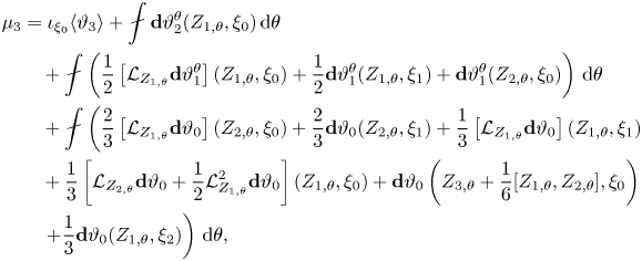 \begin{align} \mu_3 & = \iota_{\xi_0}\langle\vartheta_3 \rangle +{\unicode{x2A0F}} \mathbf{d}\vartheta_2^\theta (Z_{1,\theta},\xi_0)\,\textrm{d}\theta \nonumber\\ &\quad + {\unicode{x2A0F}}\left(\frac{1}{2}\left[{\mathcal{L}}_{Z_{1,\theta}}\mathbf{d}\vartheta_1^\theta\right] (Z_{1,\theta},\xi_0) + \frac{1}{2} \mathbf{d}\vartheta_1^\theta(Z_{1,\theta},\xi_1)+ \mathbf{d}\vartheta_1^\theta(Z_{2,\theta},\xi_0)\right)\,\textrm{d}\theta\nonumber\\ &\quad + {\unicode{x2A0F}}\left(\frac{2}{3} \left[{\mathcal{L}}_{Z_{1,\theta}}\mathbf{d}\vartheta_0\right] (Z_{2,\theta},\xi_0) + \frac{2}{3} \mathbf{d}\vartheta_0 (Z_{2,\theta},\xi_1) + \frac{1}{3} \left[{\mathcal{L}}_{Z_{1,\theta}}\mathbf{d}\vartheta_0\right](Z_{1,\theta},\xi_1)\right.\nonumber\\ &\quad+ \frac{1}{3}\left[{\mathcal{L}}_{Z_{2,\theta}}\mathbf{d}\vartheta_0 + \frac{1}{2}{\mathcal{L}}_{Z_{1,\theta}}^2\mathbf{d}\vartheta_0\right](Z_{1,\theta},\xi_0) + \mathbf{d}\vartheta_0\left(Z_{3,\theta} + \frac{1}{6}[Z_{1,\theta},Z_{2,\theta}],\xi_0\right)\nonumber\\ &\quad \left.+ \frac{1}{3}\mathbf{d}\vartheta_0(Z_{1,\theta},\xi_2)\right)\,\textrm{d}\theta, \end{align}
which can again be simplified using
 \begin{gather} \mathbf{d}\vartheta_2^\theta + {\mathcal{L}}_{Z_{1,\theta}}\mathbf{d}\vartheta_1^\theta + {\mathcal{L}}_{Z_{2,\theta}}\mathbf{d}\vartheta_0 + \frac{1}{2}{\mathcal{L}}_{Z_{1,\theta}}^2\mathbf{d}\vartheta_0 = \mathbf{d}\vartheta_2, \end{gather}
 \begin{gather}\iota_{\xi_2}\mathbf{d}\vartheta_0 + \iota_{\xi_1}\mathbf{d}\vartheta_1 + \iota_{\xi_0}\mathbf{d}\vartheta_2 = - \mathbf{d}\mu_2 \end{gather}
together with the identities (3.43)–(3.44), leading to
 \begin{align} \mu_3 & = \iota_{\xi_0}\langle \vartheta_3\rangle + \frac{2}{3}{\unicode{x2A0F}} \mathbf{d}\vartheta_2(Z_{1,\theta},\xi_0)\,\textrm{d}\theta\nonumber\\ &\quad + \frac{1}{3}{\unicode{x2A0F}} \mathbf{d}\vartheta_1^\theta(Z_{1,\theta},\xi_1^\theta)\,\textrm{d}\theta -\frac{1}{6}{\unicode{x2A0F}} \mathbf{d}\vartheta_1(Z_{1,\theta},\xi_1^\theta)\,\textrm{d}\theta\nonumber\\ &\quad - \frac{1}{3}{\unicode{x2A0F}} \mathbf{d}\vartheta_0(Z_{2,\theta},\xi_1^\theta)\,\textrm{d}\theta -\frac{1}{6}{\unicode{x2A0F}} \mathbf{d}\vartheta_0(Z_{1,\theta},{\mathcal{L}}_{Z_{1,\theta}}\xi_1^\theta)\,\textrm{d}\theta\nonumber\\ &\quad +{\unicode{x2A0F}}\left(\frac{2}{3}{\mathcal{L}}_{Z_{2,\theta}}\mu_1 + \frac{1}{3}{\mathcal{L}}_{Z_{2,\theta}}\mu_1^\theta + \frac{1}{6}{\mathcal{L}}^2_{Z_{1,\theta}}\mu_1^\theta + \frac{1}{3}{\mathcal{L}}_{Z_{1,\theta}}\mu_2\right)\,\textrm{d}\theta\nonumber\\ &\quad + {\unicode{x2A0F}} {\mathcal{L}}_{Z_{3,\theta} + \frac{1}{6}[Z_{1,\theta},Z_{2,\theta}]}\mu_0\,\textrm{d}\theta. \end{align}
Using the identity
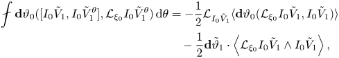 \begin{align} {\unicode{x2A0F}} \mathbf{d}\vartheta_0([I_0\tilde{V}_1,I_0\tilde{V}_1^\theta],{\mathcal{L}}_{\xi_0}I_0\tilde{V}_1^\theta)\,\textrm{d}\theta&=-\frac{1}{2}{\mathcal{L}}_{I_0\tilde{V}_1}\langle \mathbf{d}\vartheta_0({\mathcal{L}}_{\xi_0}I_0\tilde{V}_1,I_0\tilde{V}_1)\rangle \nonumber\\ &\quad - \frac{1}{2}\mathbf{d}\tilde{\vartheta}_1\cdot\left\langle {\mathcal{L}}_{\xi_0}I_0\tilde{V}_1\wedge I_0\tilde{V}_1 \right\rangle, \end{align}
together with (2.25) and (3.38), the first five integrals in (3.49) may be evaluated explicitly, resulting in the desired expression (3.17).
4. Example 1: charged particle in a magnetic field
As an example and verification test for the formulas provided by Theorem 3.5, we will now use Theorem 3.5 to recover the first two terms of the well-known adiabatic invariant series for a charged particle in a magnetic field. The nearly periodic Hamiltonian system that describes such charged particles is the ODE on  $Q\times \mathbb {R}^3$ given by
 \begin{equation} \left.\begin{gathered} \dot{\boldsymbol{v}} = \frac{1}{\epsilon}\boldsymbol{v}\times\boldsymbol{B}(\boldsymbol{x}),\\ \dot{\boldsymbol{x}} = \boldsymbol{v}, \end{gathered}\right\} \end{equation}
where  $Q\subset \mathbb {R}^3$ is an open subset representing the spatial domain, and
  $\boldsymbol {B} =\nabla \times \boldsymbol {A}$ is a magnetic field on
  $Q$. If
  $\boldsymbol {b} = \boldsymbol {B}/|\boldsymbol {B}|$ denotes the unit vector along the magnetic field then
  $V_0 = \boldsymbol {v}\times \boldsymbol {B}\boldsymbol {\cdot }\partial _{\boldsymbol {v}}$;
  $V_1 = \boldsymbol {v}\boldsymbol {\cdot } \partial _{\boldsymbol {x}}$; the limiting roto-rate vector is given by
  $\xi _0 = \boldsymbol {v}\times \boldsymbol {b}\boldsymbol {\cdot } \partial _{\boldsymbol {v}}$; the frequency function
  $\omega _0 = |\boldsymbol {B}|$; and the Hamiltonian structure is specified by the one-form
  $\vartheta _\epsilon = \boldsymbol {A}\boldsymbol {\cdot } \textrm {d}\boldsymbol {x} +\epsilon \boldsymbol {v}\boldsymbol {\cdot } \textrm {d}\boldsymbol {x}$ and the Hamiltonian
  $H_\epsilon = \epsilon \frac {1}{2}|\boldsymbol {v}|^2$. The exponential of the limiting roto-rate vector is given by
 \begin{equation} \exp(\theta\xi_0)(\boldsymbol{x},\boldsymbol{v}) = (\boldsymbol{x}, \boldsymbol{v}\boldsymbol{\cdot}\boldsymbol{b}\boldsymbol{b} + \sin\theta\boldsymbol{v}\times\boldsymbol{b} + \cos\theta\boldsymbol{b}\times(\boldsymbol{v}\times\boldsymbol{b})), \end{equation}
where  $\boldsymbol {b}$ should be evaluated at
  $\boldsymbol {x}$. Note that we have introduced the useful shorthand notation
  $\boldsymbol {u}\boldsymbol {\cdot } \partial _{\boldsymbol {x}} = u^i\partial _{x^i}$ and
  $\boldsymbol {w}\boldsymbol {\cdot }\partial _{\boldsymbol {v}} = w^i\partial _{v^i}$;
  $\partial _{\boldsymbol {x}}$ and
  $\partial _{\boldsymbol {v}}$ may be interpreted as
  $3$-component vectors whose components are partial derivative operators. Also note that the limiting roto-rate
  $\xi _0$, and therefore the full roto-rate
  $\xi _\epsilon$, is well defined for all particles, including those with field-aligned velocity vectors. This is a significant point because the usual coordinate system
  $(\boldsymbol {x},v_\parallel ,|\boldsymbol {v}_\perp |,\theta )$ used to study guiding centre dynamics has a singularity where
  $|\boldsymbol {v}_\perp |=0$.
Consider first  $\mu _0$, which according to Theorem 3.5 is given by (3.14). Because the flow of
  $\xi _0$ leaves
  $\boldsymbol {x}$ unchanged the average
  $\langle \vartheta _0\rangle = \vartheta _0 = \boldsymbol {A}\boldsymbol {\cdot } \textrm {d}\boldsymbol {x}$. Therefore
  $\mu _0 = \iota _{\xi _0}\vartheta _0 = (\boldsymbol {A}\boldsymbol {\cdot } \textrm {d}\boldsymbol {x})(\boldsymbol {v}\times \boldsymbol {b}\boldsymbol {\cdot }\partial _{\boldsymbol {v}}) =0$. This says that the adiabatic invariant series for this system is degenerate to leading order.
Next consider  $\mu _1$, which according to Theorem 3.5 is given by (3.15). Since
  $\mu _0$ vanishes, the general formula simplifies to
  $\mu _1 = \iota _{\xi _0}\langle \vartheta _1\rangle$, where
  $\vartheta _1 = \boldsymbol {v}\boldsymbol {\cdot } \textrm {d}\boldsymbol {x}$. The average of this one-form is given by
 \begin{equation} \langle \vartheta_1\rangle = {\unicode{x2A0F}} \exp(\theta\xi_0)^*\vartheta_1\,\textrm{d}\theta = {\unicode{x2A0F}} \left(\boldsymbol{v}_\theta\boldsymbol{\cdot} \textrm{d}\boldsymbol{x}\right)\,\textrm{d}\theta = (\boldsymbol{v}\boldsymbol{\cdot}\boldsymbol{b})\boldsymbol{b}\boldsymbol{\cdot} \textrm{d}\boldsymbol{x}, \end{equation}
where we have introduced the shorthand  $\boldsymbol {v}_\theta =\boldsymbol {v}\boldsymbol {\cdot }\boldsymbol {b}\boldsymbol {b} + \sin \theta \boldsymbol {v}\times \boldsymbol {b} + \cos \theta \boldsymbol {b}\times (\boldsymbol {v}\times \boldsymbol {b})$. Therefore the first-order term in the adiabatic invariant series is
  $\mu _1 = ((\boldsymbol {v}\boldsymbol {\cdot }\boldsymbol {b})\boldsymbol {b}\boldsymbol {\cdot } \textrm {d}\boldsymbol {x})(\boldsymbol {v}\times \boldsymbol {b}\boldsymbol {\cdot }\partial _{\boldsymbol {v}}) = 0$. A double degeneracy!
The calculation starts to get interesting with  $\mu _2$. Due to the double degeneracy, and the fact that
  $\vartheta _2 = 0$, the general formula (3.16) simplifies to
  $\mu _2 = \frac {1}{2}\langle \mathbf{d}\vartheta _0({\mathcal {L}}_{\xi _0}I_0\tilde {V}_1,I_0\tilde {V}_1)\rangle$. For the sake of evaluating this expression it is useful to record the following formulas for
  $V_1^\theta$,
  $I_0\tilde {V}_1^\theta$ and
  ${\mathcal {L}}_{\xi _0}I_0\tilde {V}_1^\theta$,
 \begin{align} {V}_1^\theta & =(\boldsymbol{v}\boldsymbol{\cdot}\boldsymbol{b}\boldsymbol{b})\boldsymbol{\cdot}\partial_{\boldsymbol{x}} +\frac{1}{2}\left\{([\boldsymbol{v}\times\boldsymbol{b}]\boldsymbol{\cdot}\nabla\boldsymbol{b})\times\boldsymbol{v} +2(\boldsymbol{v}\boldsymbol{\cdot}\boldsymbol{b})(\boldsymbol{b}\times\boldsymbol{\kappa})\right.\nonumber\\ &\quad\left. \times\boldsymbol{v}-(\boldsymbol{b}\times[\boldsymbol{v}_\perp\boldsymbol{\cdot}\nabla\boldsymbol{b}])\times\boldsymbol{v}\right\}\boldsymbol{\cdot}\partial_{\boldsymbol{v}}\nonumber\\ &\quad + \cos\theta\left(\boldsymbol{v}_\perp\boldsymbol{\cdot}\partial_{\boldsymbol{x}} + \left\{(\boldsymbol{b}\times [\boldsymbol{v}_\perp\boldsymbol{\cdot}\nabla\boldsymbol{b}])\times\boldsymbol{v} - (\boldsymbol{v}\boldsymbol{\cdot}\boldsymbol{b})(\boldsymbol{b}\times\boldsymbol{\kappa})\times\boldsymbol{v}\right\}\boldsymbol{\cdot}\partial_{\boldsymbol{v}}\right)\nonumber\\ &\quad + \sin\theta\left(\boldsymbol{v}\times\boldsymbol{b}\boldsymbol{\cdot} \partial_{\boldsymbol{x}}+ \left\{(\boldsymbol{v}\boldsymbol{\cdot}\boldsymbol{b})\boldsymbol{\kappa}\times\boldsymbol{v} +(\boldsymbol{b}\times[[\boldsymbol{v}\times\boldsymbol{b}]\boldsymbol{\cdot}\nabla\boldsymbol{b}])\times\boldsymbol{v}\right\}\boldsymbol{\cdot}\partial_{\boldsymbol{v}}\right)\nonumber\\ &\quad-\frac{1}{2}\cos2\theta\,\{([\boldsymbol{v}\times\boldsymbol{b}]\boldsymbol{\cdot}\nabla\boldsymbol{b})\times\boldsymbol{v}+ (\boldsymbol{b}\times[\boldsymbol{v}_\perp\boldsymbol{\cdot}\nabla\boldsymbol{b}])\times\boldsymbol{v}\}\boldsymbol{\cdot}\partial_{\boldsymbol{v}}\nonumber\\ &\quad+\frac{1}{2}\sin2\theta\,\left\{(\boldsymbol{v}_\perp\boldsymbol{\cdot}\nabla\boldsymbol{b})\times\boldsymbol{v} -(\boldsymbol{b}\times[[\boldsymbol{v}\times\boldsymbol{b}]\boldsymbol{\cdot}\nabla\boldsymbol{b}])\times\boldsymbol{v}\right\}\boldsymbol{\cdot}\partial_{\boldsymbol{v}}, \end{align}
 \begin{align} I_0\tilde{V}_1^\theta & = -|\boldsymbol{B}|^{-1}[\boldsymbol{v}_\perp\cos\theta + \boldsymbol{v}\times\boldsymbol{b}\sin\theta]\boldsymbol{\cdot}\nabla\ln|\boldsymbol{B}| (\boldsymbol{v}\times\boldsymbol{b})\boldsymbol{\cdot}\partial_{\boldsymbol{v}}\nonumber\\ &\quad + |\boldsymbol{B}|^{-1}\sin\theta\left(\boldsymbol{v}_\perp\boldsymbol{\cdot}\partial_{\boldsymbol{x}} + \left\{(\boldsymbol{b}\times [\boldsymbol{v}_\perp\boldsymbol{\cdot}\nabla\boldsymbol{b}])\times\boldsymbol{v} - (\boldsymbol{v}\boldsymbol{\cdot}\boldsymbol{b})(\boldsymbol{b}\times\boldsymbol{\kappa})\times\boldsymbol{v}\right\}\boldsymbol{\cdot}\partial_{\boldsymbol{v}}\right)\nonumber\\ &\quad -|\boldsymbol{B}|^{-1} \cos\theta\left(\boldsymbol{v}\times\boldsymbol{b}\boldsymbol{\cdot}\partial_{\boldsymbol{x}} +\left\{(\boldsymbol{v}\boldsymbol{\cdot}\boldsymbol{b})\boldsymbol{\kappa}\times\boldsymbol{v} +(\boldsymbol{b}\times[[\boldsymbol{v}\times\boldsymbol{b}]\boldsymbol{\cdot}\nabla\boldsymbol{b}])\times\boldsymbol{v}\right\}\boldsymbol{\cdot}\partial_{\boldsymbol{v}}\right)\nonumber\\ &\quad-\frac{1}{4}|\boldsymbol{B}|^{-1}\sin2\theta\,\{([\boldsymbol{v}\times\boldsymbol{b}]\boldsymbol{\cdot}\nabla\boldsymbol{b})\times\boldsymbol{v} +(\boldsymbol{b}\times[\boldsymbol{v}_\perp\boldsymbol{\cdot}\nabla\boldsymbol{b}])\times\boldsymbol{v}\}\boldsymbol{\cdot}\partial_{\boldsymbol{v}}\nonumber\\ &\quad-\frac{1}{4}|\boldsymbol{B}|^{-1}\cos2\theta\,\left\{(\boldsymbol{v}_\perp\boldsymbol{\cdot}\nabla\boldsymbol{b})\times\boldsymbol{v} -(\boldsymbol{b}\times[[\boldsymbol{v}\times\boldsymbol{b}]\boldsymbol{\cdot}\nabla\boldsymbol{b}])\times\boldsymbol{v}\right\}\boldsymbol{\cdot}\partial_{\boldsymbol{v}}, \end{align}
 \begin{align} {\mathcal{L}}_{\xi_0}I_0\tilde{V}_1^\theta & = -|\boldsymbol{B}|^{-1}[\boldsymbol{v}\times\boldsymbol{b}\cos\theta-\boldsymbol{v}_\perp\sin\theta ]\boldsymbol{\cdot}\nabla\ln|\boldsymbol{B}| (\boldsymbol{v}\times\boldsymbol{b})\boldsymbol{\cdot}\partial_{\boldsymbol{v}}\nonumber\\ &\quad +|\boldsymbol{B}|^{-1}\cos\theta\left(\boldsymbol{v}_\perp\boldsymbol{\cdot}\partial_{\boldsymbol{x}} + \left\{(\boldsymbol{b}\times [\boldsymbol{v}_\perp\boldsymbol{\cdot}\nabla\boldsymbol{b}])\times\boldsymbol{v} - (\boldsymbol{v}\boldsymbol{\cdot}\boldsymbol{b})(\boldsymbol{b}\times\boldsymbol{\kappa})\times\boldsymbol{v}\right\}\boldsymbol{\cdot}\partial_{\boldsymbol{v}}\right)\nonumber\\ &\quad +|\boldsymbol{B}|^{-1} \sin\theta\left(\boldsymbol{v}\times\boldsymbol{b}\boldsymbol{\cdot}\partial_{\boldsymbol{x}} +\left\{(\boldsymbol{v}\boldsymbol{\cdot}\boldsymbol{b})\boldsymbol{\kappa}\times\boldsymbol{v} +(\boldsymbol{b}\times[[\boldsymbol{v}\times\boldsymbol{b}]\boldsymbol{\cdot}\nabla\boldsymbol{b}])\times\boldsymbol{v}\right\}\boldsymbol{\cdot}\partial_{\boldsymbol{v}}\right)\nonumber\\ &\quad-\frac{1}{2}|\boldsymbol{B}|^{-1}\cos2\theta\,\{([\boldsymbol{v}\times\boldsymbol{b}]\boldsymbol{\cdot}\nabla\boldsymbol{b})\times\boldsymbol{v} +(\boldsymbol{b}\times[\boldsymbol{v}_\perp\boldsymbol{\cdot}\nabla\boldsymbol{b}])\times\boldsymbol{v}\}\boldsymbol{\cdot}\partial_{\boldsymbol{v}}\nonumber\\ &\quad+\frac{1}{2}|\boldsymbol{B}|^{-1}\sin2\theta\,\left\{(\boldsymbol{v}_\perp\boldsymbol{\cdot}\nabla\boldsymbol{b})\times\boldsymbol{v} -(\boldsymbol{b}\times[[\boldsymbol{v}\times\boldsymbol{b}]\boldsymbol{\cdot}\nabla\boldsymbol{b}])\times\boldsymbol{v}\right\}\boldsymbol{\cdot}\partial_{\boldsymbol{v}} , \end{align}
where  $\boldsymbol {\kappa } = \boldsymbol {b}\boldsymbol {\cdot }\nabla \boldsymbol {b}$ is the field-line curvature and
  $\boldsymbol {v}_\perp = \boldsymbol {b}\times (\boldsymbol {v}\times \boldsymbol {b})$ is the projection of the velocity into the plane perpendicular to the magnetic field. If
  $U = U_{\boldsymbol {x}}\boldsymbol {\cdot }\partial _{\boldsymbol {x}} + U_{\boldsymbol {v}}\boldsymbol {\cdot }\partial _{\boldsymbol {v}}$ and
  $W = W_{\boldsymbol {x}}\boldsymbol {\cdot }\partial _{\boldsymbol {x}} + W_{\boldsymbol {v}}\boldsymbol {\cdot }\partial _{\boldsymbol {v}}$ are any two vector fields on
  $Q\times \mathbb {R}^3$ then
  $\mathbf{d}\vartheta _0(U,V) = \boldsymbol {B}\boldsymbol {\cdot } U_{\boldsymbol {x}}\times W_{\boldsymbol {x}}$. In particular, when
  $U$ is given by (4.6) and
  $W$ is given by (4.5) the expression becomes
  $\mathbf{d}\vartheta _0({\mathcal {L}}_{\xi _0}I_0\tilde {V}_1^\theta ,I_0\tilde {V}_1^\theta ) = |\boldsymbol {B}|^{-1}|\boldsymbol {v}\times \boldsymbol {b}|^2$ for each
  $\theta \in S^1$. It follows that
  $\mu _2 = \frac {1}{2}|\boldsymbol {B}|^{-1}|\boldsymbol {v}\times \boldsymbol {b}|^2$, which is the familiar expression for the leading term in the magnetic moment series. Note that because
  $\mu _2$ is the first non-trivial term in the adiabatic invariant series for this system standard convention is to refer to this quantity as
  $\mu _0$ rather than
  $\mu _2$. We have not adopted this convention in this article because not all nearly periodic Hamiltonian systems exhibit the double degeneracy
  $\mu _0 = \mu _1 = 0$.
Finally, consider  $\mu _3$, which should give the first correction to the magnetic moment. Because
  $\vartheta _2 = \vartheta _3 = 0$,
  $V_2 = 0$,
  $\mu _0 = 0$ and
  $\mu _1 = 0$ the general formula (3.17) reduces to
 \begin{align} \mu_3& = - \frac{1}{3}\langle \mathbf{d}\vartheta_1({\mathcal{L}}_{\xi_0}I_0\tilde{V}_1,I_0\tilde{V}_1)\rangle\nonumber\\ &\quad + \frac{1}{3}\left\langle \iota_{{\mathcal{L}}_{\xi_0}I_0\tilde{V}_1}\mathbf{d}\vartheta_1\right\rangle(I_0\tilde{V}_1) - \frac{1}{6}\langle \mathbf{d}\vartheta_0([{\mathcal{L}}_{\xi_0}I_0\tilde{V}_1,I_0\tilde{V}_1], I_0\tilde{V}_1)\rangle \nonumber\\ &\quad + \frac{1}{6}\mathbf{d}\vartheta_0(\langle [{\mathcal{L}}_{\xi_0}I_0\tilde{V}_1,I_0\tilde{V}_1]\rangle,I_0\tilde{V}_1) \nonumber\\ &\quad + \frac{1}{3}\langle \mathbf{d}\vartheta_0({\mathcal{L}}_{\xi_0}I_0\tilde{V}_1, I_0[I_0\tilde{V}_1,\langle V_1\rangle])\rangle+\frac{1}{6}\langle \mathbf{d}\vartheta_0({\mathcal{L}}_{\xi_0}I_0\tilde{V}_1,I_0[I_0\tilde{V}_1,\tilde{V}_1]^{\textrm{osc}})\rangle\nonumber\\ &\quad + \frac{1}{6}\langle \langle\mathbf{d}\vartheta_1 \rangle({\mathcal{L}}_{\xi_0}I_0\tilde{V}_1,I_0\tilde{V}_1)\rangle - \frac{1}{3}{\mathcal{L}}_{I_0\tilde{V}_1}\langle \mathbf{d}\vartheta_0({\mathcal{L}}_{\xi_0}I_0\tilde{V}_1,I_0\tilde{V}_1) \rangle. \end{align}
In order to eliminate the possibility of human error in evaluating each of the terms in (4.7) we used the vector calculus simplification tool VEST to perform the calculation. VEST was originally developed in Squire, Burby & Qin (Reference Squire, Burby and Qin2014) for the purpose of implementing the automatic calculation of the guiding centre calculation in Burby, Squire & Qin (Reference Burby, Squire and Qin2013), and is therefore admirably suited to the present calculation. The final result is
 \begin{align} \mu_3 &= \mu_0\frac{(\boldsymbol{b}\times\boldsymbol{v})\boldsymbol{\cdot} \nabla |\boldsymbol{B}|}{|\boldsymbol{B}|^2} + \frac{1}{4}\frac{(\boldsymbol{v}\boldsymbol{\cdot}\boldsymbol{b})\,\boldsymbol{v}\boldsymbol{\cdot}\nabla\boldsymbol{b}\boldsymbol{\cdot}(\boldsymbol{v}\times\boldsymbol{b})}{|\boldsymbol{B}|^2} \nonumber\\ &\quad -\frac{3}{4}\frac{(\boldsymbol{v}\boldsymbol{\cdot}\boldsymbol{b})\, (\boldsymbol{v}\times\boldsymbol{b})\boldsymbol{\cdot}\nabla\boldsymbol{b}\boldsymbol{\cdot}\boldsymbol{v} }{|\boldsymbol{B}|^2} - \frac{5}{4}\frac{(\boldsymbol{v}\boldsymbol{\cdot}\boldsymbol{v})^2\,\boldsymbol{\kappa}\boldsymbol{\cdot}(\boldsymbol{v}\times\boldsymbol{b})}{|\boldsymbol{B}|^2}, \end{align}
which agrees with the formula from Weyssow & Balescu (Reference Weyssow and Balescu1986).
5. Example 2: an adiabatic invariant for nearly periodic magnetic fields
KAM theory reveals much about the structure of toroidal magnetic fields used for the purpose of magnetic confinement fusion. Perhaps most significantly it provides the following stability result. If the true magnetic field within a device is close to a fiducial field with nested toroidal flux surfaces, and the magnetic shear of the fiducial field is bounded away from zero, then the true field will have nearly the same measure of flux surfaces as the fiducial field. In the narrow gaps between the surviving flux surfaces, deterministic chaos reigns.
On the other hand, KAM theory has less to say when the fiducial, unperturbed field has vanishing shear, particularly when the rotational transform is constant and rational. For example, Moser (Reference Moser1973) requires perturbations to be small relative to shear. Herman (Reference Herman1983) allows for small shear, but requires strongly irrational rotational transform and introduces an external parameter as a substitute for the non-vanishing shear condition. (The external parameter trick is due to Rússmann, and explained for example in Rüssmann (Reference Rüssmann1976).) Non-vanishing shear ensures that many of the unperturbed flux surfaces possess strongly non-resonant (i.e. strongly irrational) rotational transform. Such non-resonant tori survive perturbations with relative ease, and provide the true, perturbed magnetic field with a source of KAM tori. When all of the fiducial field lines are closed, however, this well of non-resonant unperturbed flux surfaces runs dry. Even though the unperturbed field contains many (non-unique) flux surfaces, each of these is strongly resonant. It would therefore seem that closed-line fields should easily be blown apart by most perturbations.
In order to examine the susceptibility of closed field lines to magnetic perturbations, suppose that  $\boldsymbol {B}_\epsilon = \nabla \times \boldsymbol {A}_\epsilon$ is a non-vanishing magnetic field for each
  $\epsilon \in \mathbb {R}$. The field
  $\boldsymbol {B}_\epsilon$ has nearly closed field lines if
  $\boldsymbol {A}_\epsilon$ depends smoothly on
  $\epsilon$ and each field line of
  $\boldsymbol {B}_0$ is closed. A remarkable property of such a magnetic field is that the associated field-line dynamical system
  $\dot {\boldsymbol {x}} = \epsilon ^{-1}\boldsymbol {B}_\epsilon (\boldsymbol {x})$ comprises a nearly periodic Hamiltonian system on
  $Z = Q$, the field-line container. The frequency function is given by
 \begin{equation} \frac{1}{\omega_0(\boldsymbol{x})} = \frac{1}{2{\rm \pi}}\oint_{\ell_0(\boldsymbol{x})}\frac{\textrm{d}\ell}{|\boldsymbol{B}|}, \end{equation}
where  $\ell _0(\boldsymbol {x})$ is the unique
  $\boldsymbol {B}_0$-line that contains the point
  $\boldsymbol {x}\in Q$; the limiting roto-rate vector is
  $\xi _0 = \boldsymbol {B}_0/\omega _0$; the presymplectic form is
  $-\mathbf{d}(\boldsymbol {A}_\epsilon \boldsymbol {\cdot } \textrm {d}\boldsymbol {x}) = -\iota _{\boldsymbol {B}_\epsilon }\textrm {d}^3\boldsymbol {x}$; and the Hamiltonian is
  $H_\epsilon =0$. Therefore the general theory outlined in Kruskal (Reference Kruskal1962), as well as the rest of this article, guarantees the existence of a field-line adiabatic invariant
  $\mu _\epsilon$ for
  $\boldsymbol {B}_\epsilon$ when
  $\epsilon$ is small. Since such an adiabatic invariant defines approximate flux surfaces (surfaces that field lines traverse many times before possibly wandering away), magnetic fields with nearly closed lines of force enjoy much more stability than KAM theory, and in particular that theory's assumption of non-vanishing shear, suggests. Note, in particular, that existence of the field-line adiabatic invariant
  $\mu _\epsilon$ does not require the perturbation
  $\boldsymbol {B}_\epsilon - \boldsymbol {B}_0$ to be non-resonant.
The robustness of magnetic fields with nearly closed field lines is consistent with previous experimental and theoretical analyses of magnetic fields and fluid flows with regions of low or sign-reversing shear. See for example Firpo & Constantinescu (Reference Firpo and Constantinescu2011) for a fusion-oriented study and del Castillo-Negrete & Morrison (Reference del Castillo-Negrete and Morrison1992) for an investigation of analogous ideas in the context of sheared fluid flow. In any low-shear region, a rational number  $q/p$ may be found that uniformly approximates the unperturbed field's rotational transform
  $\iota (\psi )$. By writing
  $\iota (\psi ) = q/p + (\iota (\psi ) - q/p)$, the unperturbed magnetic field may then be expressed as a field with closed lines plus a correction that is proportional to the shear. Because the shear is small by hypothesis it is therefore natural to lump the correction term
  $\delta \iota (\psi ) =\iota (\psi ) - q/p$ together with any magnetic perturbations that may be present. In this manner the magnetic field within a region of small shear may be expressed as a magnetic field with nearly closed field lines. The field-line dynamics within a low-shear region therefore possesses an adiabatic invariant
  $\mu _\epsilon$. Moreover, approximate level sets of
  $\mu _\epsilon$ may be used to quickly predict the field-line transport effects, deleterious or not, of the perturbation. This approach to understanding the impacts of perturbations on low-shear magnetic fields appears to have gone largely unnoticed; the preferred approach has been the more cumbersome and obtuse action-angle formalism.
In order to gain insight into the significance of the adiabatic flux surfaces defined by  $\mu _\epsilon$, consider the formulas for
  $\mu _\epsilon$ provided by Theorem 3.5. According to (3.14) the coefficient
  $\mu _0=\text {const.}$ since
  $\mathbf{d}\mu _0 = -\iota _{\xi _0}\mathbf{d}\vartheta _0 = \omega _0^{-1}\iota _{\boldsymbol {B}_0}\iota _{\boldsymbol {B}_0}\textrm {d}^3\boldsymbol {x} = 0$. Therefore the first possibly non-trivial coefficient is
  $\mu _1 = \iota _{\xi _0}\langle \vartheta _1\rangle$. Apparently the value of
  $\mu _1$ at
  $\boldsymbol {x}\in Q$ may be written as the line integral
  $\mu _1(\boldsymbol {x}) = (2{\rm \pi} )^{-1}\oint _{\ell _0(\boldsymbol {x})}\boldsymbol {A}_1\boldsymbol {\cdot } \textrm {d}\boldsymbol {x}$, with
  $\ell _0(\boldsymbol {x})$ defined as above and oriented so that
  $\boldsymbol {B}(\boldsymbol {x})$ is a positive basis for
  $T_{\boldsymbol {x}}\ell _0(\boldsymbol {x})$. This quantity can be understood as a magnetic flux as follows. Suppose that
  $Q$ is path connected, fix
  $\boldsymbol {x}_0\in Q$ and define the constant
  $\mu ^*_\epsilon = (2{\rm \pi} )^{-1}\oint _{\ell _0(\boldsymbol {x}_0)}\boldsymbol {A}_\epsilon \boldsymbol {\cdot } \textrm {d}\boldsymbol {x}$. The quantity
  $\bar {\mu }_\epsilon = \mu _\epsilon - \mu _\epsilon ^*$ is an adiabatic invariant since it differs from
  $\mu _\epsilon$ by a constant. The first non-zero coefficient of
  $\bar {\mu }_\epsilon$ is
  $\bar {\mu }_1(\boldsymbol {x}) = \mu _1(\boldsymbol {x}) - \mu _1^*$, which is, up to a constant, the same as
  $\mu _1$. Let
  $\boldsymbol {x}(\lambda )$ be a curve in
  $Q$ with,
  $\partial _\lambda \boldsymbol {x}(\lambda )\neq 0$,
  $\boldsymbol {x}(0) = \boldsymbol {x}_0$, and
  $\boldsymbol {x}(1) = \boldsymbol {x}$. Set
  $R_0(\boldsymbol {x}) = \bigcup _{\lambda \in [0,1]}\ell _0(\boldsymbol {x}(\lambda ))$. Note that
  $R_0(\boldsymbol {x})$ is a flux ribbon for
  $\boldsymbol {B}_0$ because it is a union of
  $\boldsymbol {B}_0$-lines. Now apply Stokes’ theorem according to
 \begin{align} \bar{\mu}_1(\boldsymbol{x})& = \frac{1}{2{\rm \pi}}\oint_{\ell_0(\boldsymbol{x})}\boldsymbol{A}_1\boldsymbol{\cdot} \textrm{d}\boldsymbol{x} - \frac{1}{2{\rm \pi}}\oint_{\ell_0(\boldsymbol{x}_0)}\boldsymbol{A}_1\boldsymbol{\cdot} \textrm{d}\boldsymbol{x}\nonumber\\ & = \frac{1}{2{\rm \pi}}\int_{R_0(\boldsymbol{x})}\boldsymbol{B}_1\boldsymbol{\cdot} \textrm{d}\boldsymbol{S}, \end{align}
where  $R_0(\boldsymbol {x})$ is oriented so that
  $(\partial _\lambda \boldsymbol {x}(\lambda ),\boldsymbol {B}(\boldsymbol {x}(\lambda ))$ is a positive basis for
  $T_{\boldsymbol {x}(\lambda )}R_0(\boldsymbol {x})$. This shows that, up to an unimportant additive constant,
  $\mu _1(\boldsymbol {x})$ is equal to the (normalized) flux of
  $\boldsymbol {B}_1$ through any flux ribbon
  $R_0(\boldsymbol {x})$ whose boundary is
  $\partial R_0(\boldsymbol {x}) = \ell _0(\boldsymbol {x})\cup \ell _0(\boldsymbol {x}_0)$. If
  $\boldsymbol {B}_0$ contains a single magnetic axis
  $L$ then it is permissible to set
  $\ell _0(\boldsymbol {x}_0) = L$. In this special case
  $2{\rm \pi} \bar {\mu }_1$ is a perturbed poloidal flux.
The approximate flux surfaces defined by the level sets of  $\mu _1$ (or equivalent
  $\bar {\mu }_1$) determine how well field lines are confined within
  $Q$. The most favourable case for confinement occurs when the
  $\mu _1$-surfaces are nested tori contained in
  $Q$, but more exotic foliations may occur depending on the form of the perturbation
  $\boldsymbol {B}_1$. For example, let
  $\boldsymbol {B}_\epsilon = \boldsymbol {B}_0 + \epsilon \,\boldsymbol {B}_1$ with
  $\boldsymbol {B}_0 = B_0 (R_0/R)\boldsymbol {e}_{\phi }$ a tokamak vacuum field and
  $\boldsymbol {B}_1 = \alpha \nabla \psi \times \nabla \phi$. Here,
  $(R,\phi ,Z)$ are standard cylindrical coordinates,
  $\psi$ is an arbitrary function, and
  $\alpha$ is a constant. The function
  $\mu _1$ is then
 \begin{equation} \mu_1(R,\phi,Z) = \alpha\frac{1}{2{\rm \pi}}\int_0^{2{\rm \pi}}\psi(R,\bar{\phi},Z)\,\textrm{d}\bar{\phi} = \alpha\langle \psi\rangle(R,Z), \end{equation}
where the angle brackets denote an azimuthal average. In this example adiabatic flux surfaces are surfaces of revolution with poloidal cross-sections given by level sets of  $\langle \psi \rangle (R,Z)$. If
  $\psi (R,Z) = (R - R_0)^2 + Z^2$ the poloidal cross-sections are nested circles centred at
  $(R,Z) = (R_0,0)$, indicating confinement. However, if
  $\psi (R,Z) = (R-R_0)Z$ the cross-sections are hyperbolas, indicating no such confinement.
6. Conclusion
In this article, we have derived and verified general coordinate-independent expressions for the adiabatic invariant associated with a nearly periodic Hamiltonian system. These formulas are summarized in Theorem 3.5. As a byproduct of our derivation, we have also derived coordinate-independent expressions for the roto-rate vector associated with a possibly non-Hamiltonian nearly periodic system. These formulas are summarized in Theorem 2.11. Using these formulas, adiabatic invariants may be computed more efficiently and directly than prior procedure-based methods. It is worth emphasizing that none of our results imply convergence of the formal power series that define the roto-rate vector and the adiabatic invariant. In fact, Krikorian (Reference Krikorian2019) has recently proved that the Birkhoff normal form near a diophantine KAM torus generically diverges.
A goal of future work will be to apply our results to infinite dimensional systems, especially systems with slow manifolds such as ideal magnetohydrodynamics, Burby (Reference Burby2017), kinetic magnetohydrodynamics, Burby & Sengupta (Reference Burby and Sengupta2018) and Lorentz loop dynamics, Burby (Reference Burby2020). See Burby & Klotz (Reference Burby and Klotz2020) for an in-depth discussion of the role of slow manifolds in plasma physics. Just as Cotter & Reich (Reference Cotter and Reich2004) shows that the long-time persistence of quasigeostrophic balance in non-dissipative geophysical fluid flows may be explained by finding an appropriate adiabatic invariant, adiabatic invariants in these plasma-dynamical systems may explain subtle notions such as the persistence time scale for gyrotropy in strongly magnetized plasmas. The key concept underlying the results of Cotter & Reich (Reference Cotter and Reich2004) is the identification of quasigeostrophic dynamics with motion on a slow manifold. We remark that the relationship between slow manifolds and quasigeostrophic balance was established previously in Lorenz (Reference Lorenz1986, Reference Lorenz1992) and Lorenz & Krishnamurthy (Reference Lorenz and Krishnamurthy1987).
Acknowledgements
Research presented in this article was supported by the Los Alamos National Laboratory LDRD program under project number 20180756PRD4. Support for J.S. was provided by Rutherford Discovery Fellowship RDF-U001804 and Marsden Fund grant UOO1727, which are managed through the Royal Society Te Apārangi.
Declaration of interests
The authors report no conflict of interest.
Appendix A. How-to guide for the new formulas
In this appendix we provide explicit details on how to practically compute the various terms in (3.14)–(3.17).
As written, these formulas involve vector fields like  $V$, one-forms like
  $\vartheta$, and two-forms like
  $\mathbf{d}\vartheta$. For those unfamiliar with exterior calculus, the index-notation equivalents of these objects are summarized as follows:
 \begin{gather} V\leftrightarrow V^i\quad\text{(vector fields)}, \end{gather}
 \begin{gather}\vartheta \leftrightarrow \vartheta_i\quad\text{(one-forms)}, \end{gather}
 \begin{gather}\mathbf{d}\vartheta \leftrightarrow (\mathbf{d}\vartheta)_{ij}\quad \text{(two-forms)}. \end{gather}
The components of a two-form like  $\mathbf{d}\vartheta$ are related to the components of
  $\vartheta$ according to
 \begin{equation} (\mathbf{d}\vartheta)_{ij} = \partial_i\vartheta_j - \partial_j\vartheta_i, \end{equation}
and are therefore anti-symmetric. Actually all two-forms are antisymmetric. A one-form  $\vartheta$ can be contracted with a single vector field
  $V$ in order to produce a scalar field
  $\vartheta (V)$. A two-form
  $\mathbf{d}\vartheta$ can be contracted with two vector fields
  $V_1,V_2$ in order to produce a scalar field,
  $\mathbf{d}\vartheta (V_1,V_2)$. In index notation these contraction operations are summarized as follows,
 \begin{gather} \vartheta(V) = \vartheta_i V^i, \end{gather}
 \begin{gather}\mathbf{d}\vartheta(V_1,V_2) = (\mathbf{d}\vartheta)_{ij} V_1^i V_2^j. \end{gather}
A two-form  $\mathbf{d}\vartheta$ may also be contracted on the left with a single vector field
  $V$ to obtain a one-form
  $\iota _V\mathbf{d}\vartheta$ given by
 \begin{equation} (\iota_V\mathbf{d}\vartheta)_i = V^j(\mathbf{d}\vartheta)_{ji}. \end{equation}
 As for calculus, there are two important operations that must be handled. The commutator of two vector fields  $[V_1,V_2]$ is given by
 \begin{equation} [V_1,V_2]^i = V_1^j\partial_j V_2^i - V_2^j\partial_j V_1^i. \end{equation}
The Lie derivative of a scalar  $\mu$ along a vector field
  $V$,
$V$,  ${\mathcal {L}}_V\mu$, is given by
 \begin{equation} {\mathcal{L}}_V\mu = V^i\partial_i\mu. \end{equation}
 One non-trivial operation that must be performed when evaluating the formulas (3.14)–(3.17) is the  $U(1)$-average, denoted
  $\langle \cdot \rangle$. In order to carry out this operation analytically it is necessary to have an explicit expression for the phase-space mappings
  $\zeta _\theta :z\mapsto \exp (\theta \xi _0)(z)\equiv \zeta _\theta (z)$. Practically speaking, the value of
  $\exp (\theta \xi _0)(z)$ is
  $z(\theta )$, where
  $z(\theta )$ is the unique solution of the ODE
  $\partial _\theta z(\theta ) = \xi _0(z(\theta ))$ with
  $z(0) = z$. Therefore knowledge of the mapping
  $\zeta _\theta$ is tantamount to knowledge of the general solution of the ODE defined by
  $\xi _0$. Notice that
  $\xi _0$-trajectories are just reparameterizations of the leading-order dynamical trajectories
  $\dot {z} = V_0(z)$. It may be helpful to find a coordinate system where
  $\xi _0$ is simple in order to find an explicit expression
  $\zeta _\theta$. Two examples of
  $\zeta _\theta (z)$ were given in the text. Once
  $\zeta _\theta (z)$ is known, the
  $U(1)$-average can be applied to any tensor, in particular vector fields
  $V$ and one-forms
  $\vartheta$. In components, the relevant formulas are
 \begin{gather} \langle V\rangle^i(z) = {\unicode{x2A0F}} V^j(\zeta_\theta(z))\,\partial_j\zeta^i_{-\theta}(\zeta_\theta(z)) \,\textrm{d}\theta, \end{gather}
 \begin{gather}\langle \vartheta\rangle_i(z) ={\unicode{x2A0F}} \vartheta_j(\zeta_\theta(z))\,\partial_i\zeta_\theta^j(z)\,\textrm{d}\theta. \end{gather}
Because the  $U(1)$-average commutes with the exterior derivative,
  $\mathbf{d}$, the average of a two-form like
  $\mathbf{d}\vartheta$ may be computed by first finding
  $\langle \vartheta \rangle$ using (A 11) and then computing
  $\mathbf{d}\langle \vartheta \rangle = \langle \mathbf{d}\vartheta \rangle$ using (A 4).
The least non-trivial operation encountered in (3.14)–(3.17) is the operator  $I_0 = ({\mathcal {L}}_{V_0})^{-1}$. In a rough sense this operator ‘integrates along unperturbed orbits’. The easiest way to compute
  $I_0\tilde {V}$ for a fluctuating vector field
  $\tilde {V}$ is to use the following Fourier-series-based trick. First compute
  $\tilde {V}^\theta = \zeta _\theta ^*\tilde {V}$, which in components is given by
 \begin{equation} \tilde{V}^{\theta i}(z) = \tilde{V}^j(\zeta_\theta(z))\partial_j\zeta^i_{-\theta}(\zeta_\theta(z)). \end{equation}
Because  $\zeta _\theta (z)$ is
  $2{\rm \pi}$-periodic in
  $\theta$ the component
  $\tilde {V}^{\theta i}(z)$ must have a Fourier series expansion
 \begin{equation} \tilde{V}^{\theta i}(z) = \sum_{n\in\mathbb{Z}} \tilde{V}^i_n(z)\,\textrm{e}^{\textrm{i}n\theta}, \end{equation}
where the Fourier coefficients  $\tilde {V}^i_n(z)$ are complex-valued functions of
  $z$. We can use these Fourier coefficients to help solve the problem
  ${\mathcal {L}}_{V_0}\tilde {U} = \tilde {V}$ for
  $\tilde {U}$ given
  $\tilde {V}$. Note that finding
  $\tilde {U}$ is equivalent to finding
  $I_0\tilde {V}$. To see how, apply the pullback
  $\zeta _\theta ^*$ to the equation
  ${\mathcal {L}}_{V_0}\tilde {U} = \tilde {V}$ to obtain
  ${\mathcal {L}}_{V_0}\tilde {U}^\theta = \tilde {V}^\theta$. The LHS of this equation simplifies considerably by noting
  ${\mathcal {L}}_{V_0}\tilde {U}^\theta = -{\mathcal {L}}_{\tilde {U}^\theta }V_0 =-{\mathcal {L}}_{\tilde {U}^\theta }(\omega _0 \xi _0) = -\xi _0\,{\mathcal {L}}_{\tilde {U}^\theta }\omega _0 +\omega _0{\mathcal {L}}_{\xi _0}\tilde {U}^\theta = -\xi _0 {\mathcal {L}}_{\tilde {U}^\theta }\omega _0 +\omega _0\partial _\theta \tilde {U}^\theta$. In components this identity may be written
 \begin{equation} ({\mathcal{L}}_{V_0}\tilde{U}^\theta)^i = -\tilde{U}^{\theta j}\partial_j\omega_0\xi^i + \omega_0\partial_\theta\tilde{U}^{\theta i}. \end{equation}
Therefore the Fourier components of the equation  ${\mathcal {L}}_{V_0}\tilde {U}^\theta = \tilde {V}^\theta$ read
 \begin{equation} -\tilde{U}^{ j}_n\partial_j\omega_0\xi^i + \textrm{i}n\omega_0\tilde{U}^{ i}_n = \tilde{V}^i_n. \end{equation}
This infinite sequence of algebraic equations may be solved by hand, leading to the following formula for  $\tilde {U}^i_n$,
 \begin{equation} \tilde{U}^i_n = \xi^i \frac{\tilde{V}^j_n \partial_j\omega_0}{(\textrm{i}n\omega_0)^2} + \frac{\tilde{V}_n^i}{\textrm{i}n\omega_0}. \end{equation}
Since  $\tilde {U}^\theta$ is equal to
  $\tilde {U} = I_0\tilde {V}$ when
  $\theta = 0$, it follows that
  $I_0$ is determined by the formula
 \begin{equation} (I_0\tilde{V})^i = \sum_{n\in\mathbb{Z}} \xi^i \frac{\tilde{V}^j_n \partial_j\omega_0}{(\textrm{i}n\omega_0)^2} +\sum_{n\in\mathbb{Z}} \frac{\tilde{V}_n^i}{\textrm{i}n\omega_0}, \end{equation}
which can always be used to compute  $I_0$.
Appendix B. Derivation of the formula for $\xi _3$

In the proof of Theorem 2.11 we derived the general formula (2.50) for  $\tilde {\xi }_3$, but did not show how that formula can be manipulated in order to produce (2.26) for
  $\xi _3$. In this appendix we will complete the demonstration. The required manipulations are based on recursive applications of the Leibniz rule for the bracket of vector fields, i.e. the Jacobi identity. In spirit, such identities are similar to the well-known recursive Leibniz identity
 \[ e^{x}\sin x = - \frac{\textrm{d}}{\textrm{d}x}(e^x \cos x) + e^x \cos x = -\frac{\textrm{d}}{\textrm{d}x} (e^x\cos x - e^x\sin x) - e^x\sin x. \]
Starting from the general formula for  $\tilde {\xi }_3$ from Theorem 2.11,
 \begin{align*} \tilde{\xi}_3& = {\mathcal{L}}_{\xi_0} I_0\tilde{V}_3 + I_0[{\mathcal{L}}_{\xi_0} I_0\tilde{V}_1,V_2]^{\textrm{osc}} + I_0[{\mathcal{L}}_{\xi_0} I_0\tilde{V}_2,V_1]^{\textrm{osc}} \nonumber\\ &\quad + I_0\left[ {\mathcal{L}}_{\xi_0} I_0[ I_0\tilde{V}_1, \langle V_1\rangle] + \frac{1}{2}{\mathcal{L}}_{\xi_0} I_0[I_0\tilde{V}_1,\tilde{V}_1]^{\textrm{osc}} + \frac{1}{2}[{\mathcal{L}}_{\xi_0} I_0\tilde{V}_1, I_0\tilde{V}_1],V_1\right]^{\textrm{osc}} \nonumber\\ & = {\mathcal{L}}_{\xi_0} I_0\tilde{V}_3 + {\mathcal{L}}_{\xi_0} I_0[ I_0\tilde{V}_1,\langle V_2\rangle]^{\textrm{osc}} + {\mathcal{L}}_{\xi_0} I_0[ I_0\tilde{V}_2,\langle V_1\rangle]^{\textrm{osc}} \nonumber\\ &\quad+ \frac{1}{2}{\mathcal{L}}_{\xi_0} I_0[I_0\tilde{V}_2,\tilde{V}_1]^{\textrm{osc}} + \frac{1}{2} {\mathcal{L}}_{\xi_0} I_0[I_0\tilde{V}_1,\tilde{V}_2]^{\textrm{osc}}\nonumber \\ &\quad+ \frac{1}{2} [{\mathcal{L}}_{\xi_0} I_0 \tilde{V}_1,I_0\tilde{V}_2]^{\textrm{osc}}+ \frac{1}{2} [{\mathcal{L}}_{\xi_0} I_0 \tilde{V}_2,I_0\tilde{V}_1]^{\textrm{osc}}\nonumber\\ &\quad+ I_0\left[ {\mathcal{L}}_{\xi_0} I_0[ I_0\tilde{V}_1, \langle V_1\rangle] + \frac{1}{2}{\mathcal{L}}_{\xi_0} I_0[I_0\tilde{V}_1,\tilde{V}_1]^{\textrm{osc}} + \frac{1}{2}[{\mathcal{L}}_{\xi_0} I_0\tilde{V}_1, I_0\tilde{V}_1],V_1\right]^{\textrm{osc}}\nonumber\\ & = {\mathcal{L}}_{\xi_0} \left(I_0\tilde{V}_3 \!+\! I_0[ I_0\tilde{V}_1,\langle V_2\rangle]^{\textrm{osc}} \!+\!I_0[ I_0\tilde{V}_2,\langle V_1\rangle]^{\textrm{osc}}+\frac{1}{2} I_0[I_0\tilde{V}_2,\tilde{V}_1]^{\textrm{osc}} + \frac{1}{2}I_0[I_0\tilde{V}_1,\tilde{V}_2]^{\textrm{osc}} \right) \nonumber\\ &\quad + \frac{1}{2} [{\mathcal{L}}_{\xi_0} I_0 \tilde{V}_1,I_0\tilde{V}_2]^{\textrm{osc}}+ \frac{1}{2} [{\mathcal{L}}_{\xi_0} I_0 \tilde{V}_2,I_0\tilde{V}_1]^{\textrm{osc}}\nonumber\\ &\quad+ I_0\left[ {\mathcal{L}}_{\xi_0} I_0[ I_0\tilde{V}_1, \langle V_1\rangle] + \frac{1}{2}{\mathcal{L}}_{\xi_0} I_0[I_0\tilde{V}_1,\tilde{V}_1]^{\textrm{osc}} + \frac{1}{2}[{\mathcal{L}}_{\xi_0} I_0\tilde{V}_1, I_0\tilde{V}_1],\langle V_1\rangle\right]^{\textrm{osc}}\nonumber\\ &\quad+ I_0\left[ {\mathcal{L}}_{\xi_0} I_0[ I_0\tilde{V}_1, \langle V_1\rangle] + \frac{1}{2}{\mathcal{L}}_{\xi_0} I_0[I_0\tilde{V}_1,\tilde{V}_1]^{\textrm{osc}} + \frac{1}{2}[{\mathcal{L}}_{\xi_0} I_0\tilde{V}_1, I_0\tilde{V}_1],\tilde{V}_1\right]^{\textrm{osc}}\nonumber\\ & = {\mathcal{L}}_{\xi_0} \left(I_0\tilde{V}_3 \!+\! I_0[ I_0\tilde{V}_1,\langle V_2\rangle]^{\textrm{osc}} \!+\!I_0[ I_0\tilde{V}_2,\langle V_1\rangle]^{\textrm{osc}}+\frac{1}{2} I_0[I_0\tilde{V}_2,\tilde{V}_1]^{\textrm{osc}} + \frac{1}{2}I_0[I_0\tilde{V}_1,\tilde{V}_2]^{\textrm{osc}} \right) \end{align*}
 \begin{align} &\quad+ {\mathcal{L}}_{\xi_0} I_0\left[ I_0[ I_0\tilde{V}_1, \langle V_1\rangle] + \frac{1}{2} I_0[I_0\tilde{V}_1,\tilde{V}_1]^{\textrm{osc}},\langle V_1\rangle\right]\nonumber\\ &\quad + \frac{1}{2} [{\mathcal{L}}_{\xi_0} I_0 \tilde{V}_1,I_0\tilde{V}_2]^{\textrm{osc}}+ \frac{1}{2} [{\mathcal{L}}_{\xi_0} I_0 \tilde{V}_2,I_0\tilde{V}_1]^{\textrm{osc}}+ \frac{1}{2}I_0\left[[{\mathcal{L}}_{\xi_0} I_0\tilde{V}_1, I_0\tilde{V}_1]^{\textrm{osc}},\langle V_1\rangle\right]\nonumber\\ &\quad+ I_0\left[ {\mathcal{L}}_{\xi_0} I_0[ I_0\tilde{V}_1, \langle V_1\rangle] + \frac{1}{2}{\mathcal{L}}_{\xi_0} I_0[I_0\tilde{V}_1,\tilde{V}_1]^{\textrm{osc}} + \frac{1}{2}[{\mathcal{L}}_{\xi_0} I_0\tilde{V}_1, I_0\tilde{V}_1],\tilde{V}_1\right]^{\textrm{osc}}\nonumber\\ & = {\mathcal{L}}_{\xi_0} \left(I_0\tilde{V}_3 + I_0[ I_0\tilde{V}_1,\langle V_2\rangle]^{\textrm{osc}} +I_0[ I_0\tilde{V}_2,\langle V_1\rangle]^{\textrm{osc}}+\frac{1}{2} I_0[I_0\tilde{V}_2,\tilde{V}_1]^{\textrm{osc}} + \frac{1}{2}I_0[I_0\tilde{V}_1,\tilde{V}_2]^{\textrm{osc}} \right) \nonumber\\ &\quad+ {\mathcal{L}}_{\xi_0} I_0\left[ I_0[ I_0\tilde{V}_1, \langle V_1\rangle] + \frac{1}{2} I_0[I_0\tilde{V}_1,\tilde{V}_1]^{\textrm{osc}},\langle V_1\rangle\right]\nonumber\\ &\quad + \frac{1}{2} [{\mathcal{L}}_{\xi_0} I_0 \tilde{V}_1,I_0\tilde{V}_2]^{\textrm{osc}}+ \frac{1}{2} [{\mathcal{L}}_{\xi_0} I_0 \tilde{V}_2,I_0\tilde{V}_1]^{\textrm{osc}}+ \frac{1}{2}I_0\left[[{\mathcal{L}}_{\xi_0} I_0\tilde{V}_1, I_0\tilde{V}_1]^{\textrm{osc}},\langle V_1\rangle\right]\nonumber\\ &\quad+ I_0\left[ {\mathcal{L}}_{\xi_0} I_0[ I_0\tilde{V}_1, \langle V_1\rangle] + I_0[{\mathcal{L}}_{\xi_0} I_0\tilde{V}_1,\tilde{V}_1]^{\textrm{osc}},\tilde{V}_1\right]^{\textrm{osc}}\nonumber\\ & = {\mathcal{L}}_{\xi_0} \left(I_0\tilde{V}_3 + I_0[ I_0\tilde{V}_1,\langle V_2\rangle]^{\textrm{osc}} +I_0[ I_0\tilde{V}_2,\langle V_1\rangle]^{\textrm{osc}}+\frac{1}{2} I_0[I_0\tilde{V}_2,\tilde{V}_1]^{\textrm{osc}} + \frac{1}{2}I_0[I_0\tilde{V}_1,\tilde{V}_2]^{\textrm{osc}} \right) \nonumber\\ &\quad+ {\mathcal{L}}_{\xi_0} I_0\left[ I_0[ I_0\tilde{V}_1, \langle V_1\rangle] + \frac{1}{2} I_0[I_0\tilde{V}_1,\tilde{V}_1]^{\textrm{osc}},\langle V_1\rangle\right] +\frac{1}{2}{\mathcal{L}}_{\xi_0} I_0[I_0\tilde{V}_1,[I_0\tilde{V}_1,\langle V_1\rangle]]^{\textrm{osc}}\nonumber\\ &\quad + \frac{1}{2} [{\mathcal{L}}_{\xi_0} I_0 \tilde{V}_1,I_0\tilde{V}_2]^{\textrm{osc}}+ \frac{1}{2} [{\mathcal{L}}_{\xi_0} I_0 \tilde{V}_2,I_0\tilde{V}_1]^{\textrm{osc}}+ [{\mathcal{L}}_{\xi_0} I_0[I_0\tilde{V}_1,\langle V_1\rangle ],I_0\tilde{V}_1]^{\textrm{osc}}\nonumber\\ &\quad+[I_0[{\mathcal{L}}_{\xi_0} I_0\tilde{V}_1,\tilde{V}_1]^{\textrm{osc}},I_0\tilde{V}_1]^{\textrm{osc}}+\frac{1}{3}[I_0\tilde{V}_1,[{\mathcal{L}}_{\xi_0} I_0\tilde{V}_1,I_0\tilde{V}_1]^{\textrm{osc}}]^{\textrm{osc}}\nonumber\\ &\quad -\frac{1}{3}I_0[\langle [{\mathcal{L}}_{\xi_0} I_0\tilde{V}_1,I_0\tilde{V}_1] \rangle,\tilde{V}_1] + \frac{1}{3}I_0[\langle [{\mathcal{L}}_{\xi_0} I_0\tilde{V}_1,\tilde{V}_1]\rangle, I_0\tilde{V}_1]\nonumber\\ &\quad + \frac{1}{3} {\mathcal{L}}_{\xi_0} I_0[I_0\tilde{V}_1,[I_0\tilde{V}_1,\tilde{V}_1]]^{\textrm{osc}}, \end{align}
where we have used the identities
 \begin{align} & I_0[{\mathcal{L}}_{\xi_0} I_0\tilde{V}_1,V_2]^{\textrm{osc}} + I_0[{\mathcal{L}}_{\xi_0} I_0\tilde{V}_2,V_1]^{\textrm{osc}}\nonumber\\ &\quad ={\mathcal{L}}_{\xi_0} I_0[ I_0\tilde{V}_1,\langle V_2\rangle]^{\textrm{osc}} + {\mathcal{L}}_{\xi_0} I_0[ I_0\tilde{V}_2,\langle V_1\rangle]^{\textrm{osc}} \nonumber\\ &\qquad + \frac{1}{2}{\mathcal{L}}_{\xi_0} I_0[I_0\tilde{V}_2,\tilde{V}_1]^{\textrm{osc}} + \frac{1}{2} {\mathcal{L}}_{\xi_0} I_0[I_0\tilde{V}_1,\tilde{V}_2]^{\textrm{osc}}\nonumber\\ &\qquad + \frac{1}{2} [{\mathcal{L}}_{\xi_0} I_0 \tilde{V}_1,I_0\tilde{V}_2]^{\textrm{osc}}+ \frac{1}{2} [{\mathcal{L}}_{\xi_0} I_0 \tilde{V}_2,I_0\tilde{V}_1]^{\textrm{osc}}, \end{align}
 \begin{gather} {\mathcal{L}}_{\xi_0} I_0[I_0\tilde{V}_1,\tilde{V}_1]^{\textrm{osc}} = 2I_0[{\mathcal{L}}_{\xi_0} I_0\tilde{V}_1,\tilde{V}_1]^{\textrm{osc}} - [{\mathcal{L}}_{\xi_0} I_0\tilde{V}_1,I_0\tilde{V}_1]^{\textrm{osc}},\end{gather}
 \begin{align} I_0[{\mathcal{L}}_{\xi_0} I_0[I_0\tilde{V}_1,\langle V_1\rangle],\tilde{V}_1]^{\textrm{osc}} & = \frac{1}{2}{\mathcal{L}}_{\xi_0} I_0[I_0\tilde{V}_1,[I_0\tilde{V}_1,\langle V_1\rangle]]^{\textrm{osc}} + [{\mathcal{L}}_{\xi_0} I_0[I_0\tilde{V}_1,\langle V_1\rangle ],I_0\tilde{V}_1]^{\textrm{osc}}\nonumber\\ &\quad - \frac{1}{2}I_0[[{\mathcal{L}}_{\xi_0} I_0\tilde{V}_1,I_0\tilde{V}_1]^{\textrm{osc}},\langle V_1\rangle], \end{align}
and
 \begin{align} I_0[I_0[{\mathcal{L}}_{\xi_0} I_0 \tilde{V}_1,\tilde{V}_1]^{\textrm{osc}},\tilde{V}_1]^{\textrm{osc}} & = [I_0[{\mathcal{L}}_{\xi_0} I_0\tilde{V}_1,\tilde{V}_1]^{\textrm{osc}},I_0\tilde{V}_1]^{\textrm{osc}}+\frac{1}{3}[I_0\tilde{V}_1,[{\mathcal{L}}_{\xi_0} I_0\tilde{V}_1,I_0\tilde{V}_1]^{\textrm{osc}}]^{\textrm{osc}}\nonumber\\ &\quad -\frac{1}{3}I_0[\langle [{\mathcal{L}}_{\xi_0} I_0\tilde{V}_1,I_0\tilde{V}_1] \rangle,\tilde{V}_1] + \frac{1}{3}I_0[\langle [{\mathcal{L}}_{\xi_0} I_0\tilde{V}_1,\tilde{V}_1]\rangle, I_0\tilde{V}_1]\nonumber\\ &\quad + \frac{1}{3} {\mathcal{L}}_{\xi_0} I_0[I_0\tilde{V}_1,[I_0\tilde{V}_1,\tilde{V}_1]]^{\textrm{osc}}. \end{align}
Continuing to group similar terms together,
 \begin{align} \tilde{\xi}_3& = {\mathcal{L}}_{\xi_0} \left(I_0\tilde{V}_3 \!+\! I_0[ I_0\tilde{V}_1,\langle V_2\rangle]^{\textrm{osc}} \!+\!I_0[ I_0\tilde{V}_2,\langle V_1\rangle]^{\textrm{osc}}+\frac{1}{2} I_0[I_0\tilde{V}_2,\tilde{V}_1]^{\textrm{osc}} + \frac{1}{2}I_0[I_0\tilde{V}_1,\tilde{V}_2]^{\textrm{osc}} \right) \nonumber\\ &\quad + {\mathcal{L}}_{\xi_0} I_0\left[ I_0[ I_0\tilde{V}_1, \langle V_1\rangle] + \frac{1}{2} I_0[I_0\tilde{V}_1,\tilde{V}_1]^{\textrm{osc}},\langle V_1\rangle\right] +\frac{1}{2}{\mathcal{L}}_{\xi_0} I_0[I_0\tilde{V}_1,[I_0\tilde{V}_1,\langle V_1\rangle]]^{\textrm{osc}}\nonumber\\ &\quad + \frac{1}{2} [{\mathcal{L}}_{\xi_0} I_0 \tilde{V}_1,I_0\tilde{V}_2]^{\textrm{osc}}+ \frac{1}{2} [{\mathcal{L}}_{\xi_0} I_0 \tilde{V}_2,I_0\tilde{V}_1]^{\textrm{osc}}+ [{\mathcal{L}}_{\xi_0} I_0[I_0\tilde{V}_1,\langle V_1\rangle ],I_0\tilde{V}_1]^{\textrm{osc}}\nonumber\\ &\quad +[I_0[{\mathcal{L}}_{\xi_0} I_0\tilde{V}_1,\tilde{V}_1]^{\textrm{osc}},I_0\tilde{V}_1]^{\textrm{osc}}+\frac{1}{3}[I_0\tilde{V}_1,[{\mathcal{L}}_{\xi_0} I_0\tilde{V}_1,I_0\tilde{V}_1]^{\textrm{osc}}]^{\textrm{osc}}\nonumber\\ &\quad -\frac{1}{3}I_0[\langle [{\mathcal{L}}_{\xi_0} I_0\tilde{V}_1,I_0\tilde{V}_1] \rangle,\tilde{V}_1] + \frac{1}{3}I_0[\langle [{\mathcal{L}}_{\xi_0} I_0\tilde{V}_1,\tilde{V}_1]\rangle, I_0\tilde{V}_1]\nonumber\\ &\quad + \frac{1}{3} {\mathcal{L}}_{\xi_0} I_0[I_0\tilde{V}_1,[I_0\tilde{V}_1,\tilde{V}_1]]^{\textrm{osc}}\nonumber\\ & = {\mathcal{L}}_{\xi_0}\left(I_0\tilde{V}_3 + I_0[ I_0\tilde{V}_1,\langle V_2\rangle]^{\textrm{osc}} +I_0[ I_0\tilde{V}_2,\langle V_1\rangle]^{\textrm{osc}}\vphantom{\frac{1}{3}}\right.\nonumber\\ &\quad +\frac{1}{2} I_0[I_0\tilde{V}_2,\tilde{V}_1]^{\textrm{osc}}+ \frac{1}{2}I_0[I_0\tilde{V}_1,\tilde{V}_2]^{\textrm{osc}}+\frac{1}{3}I_0[I_0\tilde{V}_1,[I_0\tilde{V}_1,\tilde{V}_1]]^{\textrm{osc}}\nonumber\\ &\quad+I_0[ I_0[ I_0\tilde{V}_1, \langle V_1\rangle],\langle V_1\rangle] + \frac{1}{2}I_0[ I_0[I_0\tilde{V}_1,\tilde{V}_1]^{\textrm{osc}},\langle V_1\rangle]\nonumber\\ &\quad\left.+\frac{1}{2}I_0[I_0\tilde{V}_1,[I_0\tilde{V}_1,\langle V_1\rangle]]^{\textrm{osc}}\right)\nonumber\\ &\quad + \frac{1}{2} [{\mathcal{L}}_{\xi_0} I_0 \tilde{V}_1,I_0\tilde{V}_2]^{\textrm{osc}}+ \frac{1}{2} [{\mathcal{L}}_{\xi_0} I_0 \tilde{V}_2,I_0\tilde{V}_1]^{\textrm{osc}}+ [{\mathcal{L}}_{\xi_0} I_0[I_0\tilde{V}_1,\langle V_1\rangle ],I_0\tilde{V}_1]^{\textrm{osc}}\nonumber\\ &\quad +[I_0[{\mathcal{L}}_{\xi_0} I_0\tilde{V}_1,\tilde{V}_1]^{\textrm{osc}},I_0\tilde{V}_1]^{\textrm{osc}}+I_0[\langle [{\mathcal{L}}_{\xi_0} I_0\tilde{V}_1,\tilde{V}_1]\rangle, I_0\tilde{V}_1]\nonumber\\ &\quad +\frac{1}{3}[I_0\tilde{V}_1,[{\mathcal{L}}_{\xi_0} I_0\tilde{V}_1,I_0\tilde{V}_1]]^{\textrm{osc}}. \end{align}
Combining this expression with (2.49) for  $\langle \xi _3\rangle$ and again using the identity (B 3) gives (2.26), as desired.
