Using data to build a better EM: EM* for big data

Abstract

Existing data mining techniques, more particularly iterative learning algorithms, become overwhelmed with big data. While parallelism is an obvious and, usually, necessary strategy, we observe that both (1) continually revisiting data and (2) visiting all data are two of the most prominent problems especially for iterative, unsupervised algorithms like expectation maximization algorithm for clustering (EM-T). Our strategy is to embed EM-T into a nonlinear hierarchical data structure (heap) that allows us to (1) separate data that needs to be revisited from data that does not and (2) narrow the iteration toward the data that is more difficult to cluster. We call this extended EM-T, EM*. We show our EM* algorithm outperform EM-T algorithm over large real-world and synthetic data sets. We lastly conclude with some theoretical underpinnings that explain why EM* is successful.

1 Introduction

Big data has taken center stage in analytics. While there is no formal definition, and as many shades of interpretation as can be made from “data” and “big,” there are several themes. Chief among these is that traditional ways of processing data have become inadequate. This is witnessed in how the dozen or so traditional algorithms [2], e.g., k-means or EM, have begun to be rethought and retooled [3,4,5] to deal with data that is now too massive, too complex, produced too quickly, etc., to be effectively analyzed as we have in the past.

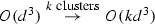
Expectation maximization (EM) is linear convergent algorithm, $\theta ^{(k+1)} = {\mathrm {M}}(\theta ^{k})$ with fix point $\theta ^* = {\mathrm {M}}(\theta ^*)$, where $\theta ^{(k)}$ is a vector of parameters on the kth iteration and $\theta ^*$ the point of convergence, recognized by its name given in [6]. The authors brought together earlier works into a broader class of optimization that dealt with incomplete data (a mix of both observed and unobserved) while providing convergence analysis. EM is simple to understand, implement and perform quite well on many kinds of data (good accuracy with relatively fast convergence). Later work [7] corrected mistakes in the original paper’s convergence analysis, but the community recognized that convergence in practice often appeared arbitrary. Subsequent focus was set upon improving our understanding of convergence and, consequently, run time with the bulk being introduced from the statistical community. While theoretically interesting, none of the solutions have left any significant impact on the original EM as it is either currently taught or used in practice. Certainly, in some circumstances, EM converges quickly. When confined to two Gaussian mixtures, for example, and the average degree of separation of the mixtures is high, the convergence is fast. While classification is linear, training can quickly overwhelm the algorithm: $O(ik(d^3 + nd^2))$ for i iterations, k Gaussians, data size n, over d dimensions.

With big data, more instances can be found that are not well modeled as Gaussian mixtures than are. And with dimensions routinely in the 100 s and data sizes in the millions, the traditional EM (EM-T) becomes increasingly impractical to use. Initialization tends not to play a significant role in the outcome of EM, provided the values are reasonable; consequently, not much attention has been paid to initialization, unlike, for example, k-means.

Rather than observed and unobserved, we distinguished what we call good and bad in this sense: Good data does not need to be revisited, while bad data does (there is an appeal to casting the problem in terms of entropy, but at this point, we have not found a sensible information-theoretic approach to our results). As an iterative algorithm, having a monotonic winnowing of the data improves the rate of convergence (or boundedness if there is not any convergence) while being at least as accurate as EM-T. Among the critical tasks were: (1) discover whether a computable, general dichotomy exists—initially we have a heuristic; (2) build additional architecture whose overhead will effectively reduce execution time; (3) examine the breadth of execution savings by varying data, e.g., size and attributes. Our results confirmed we have discovered a technique that is superior to EM-T. We call the new EM, EM*. Our results show a

• Dramatic improvement of EM* over EM-T in run time over big data, for k, n and d;

• Accuracy at least as good as EM-T in almost all the cases.

For the classical problem of $k \gg 1$, EM-T did not converge, while EM* did; the degrees of overlap were not a factor in EM-T’s failure to converge. We are presenting the deeper theoretical elements of EM* algorithm in another paper that is currently under review.

The paper continues with background on EM-T and EM* with several data sets. These data were chosen to expose the strengths and weakness of both EM-T and EM*. All of our code is in Python and the generator (multivariate) is in R. Code is available at https://github.com/hasankurban/Expectation-Maximization-Algorithm-for-Clustering. The data sets are easily accessible from https://iu.box.com/s/0teuuw2oxc42fjex9fjct886j7j6um3i.

1.1 Related and previous work

EM-T exists now as a standard tool [8,9,10] across diverse areas, e.g., [11,12,13,14] and although no current survey exists, [12, 15] together provide a good collection of various aspects of EM-T. Meng and van Dyk’s work [16], celebrating twentieth anniversary of the original EM-T paper, gives both a historical account and, to that time, approaches to faster convergence, while maintaining stability. The data set uses 100 observations.

The bulk of work relating to improving EM-T has been produced by the statistics community where, broadly, the split is among (1) employing new models (e.g., [17] segmentation of brain MR images through a hidden Markov random field model and the expectation-maximization algorithm, [18] radial basis function networks, regression weights, and the expectation-maximization algorithm, and [19] using expectation-maximization for reinforcement learning); (2) improving the accuracy (e.g., [20] improved confidence interval construction for incomplete $\hbox {r}\times \hbox {c}$ tables); and (3) increasing convergence rates and computing times. Since our work deals with the latter, we our focus will be on this branch of related work. We do point to Wu [7] who studies convergence properties of the EM-T algorithm, e.g., whether convergence is a local maximum or a stationary point of likelihood function and the sequence of the parameters predicted by EM-T when converging.

We borrow (and slightly modify) the Jamshidian and Jennrich classification of three approaches to improving speed: pure, mixed and EM-like which indicate how EM-T is modified. The most common iterative fixed point techniques compared with EM-T are Newton–Raphson (NR) and quasi-Newton (QN). Improving speed is generally through either improved gradient or increased step size; however, the most significant problem is the incomplete data log-likelihood (information matrix) that captures directly the connection between missing data and parameters. Comparing EM-T and NR for a mixed linear model, Lindstrom and Bates [21] found that the execution time for NR took four times as long than EM, while the iterations were an order of magnitude less. The paper conveys what we have found—different data produce different effective execution times without any apparent (computable) differences. When the information matrix is positive definite, NR becomes as stable as EM-T—the initial set of points that generate the convergent sequence. The QR removes the need to compute the observed information matrix and is effectively competitive with EM-T.

Pure methods, while keeping the EM-T algorithm intact, leverage tricks drawn from numerical methods in fixed point iterations. For example, the Aitken extrapolation [22] accelerates a linear convergence into quadratic by estimating a subsequent uncomputable quantity and is shown in [6, 12, 21]. While these approaches are seem relatively innocuous and promise easy gains, EM-T becomes unstable and will increasingly fail to converge.

Mixed methods, which seem to be the broadest class, include log-likelihood values themselves, but ignore the Hessian. [23] uses conjugate gradient acceleration and [24] uses QN. Using line search, unlike the pure methods, these are globally convergent. Neal et al. [25] mainly describe an incremental variant of the EM algorithm that converges faster by recalculating the distribution for only one of the unobserved variables across subsequent E-steps. Booth et al. [26] describe two extensions of the EM-T algorithm that are computationally more efficient than the EM algorithms based on Markov chain Monte Carlo algorithms and employing sampling techniques. ECM [27] is class of generalized EM algorithms and replaces M-step of the EM algorithm with computationally simpler expectation/conditional maximization (CM) steps. ECME [28] conditionally maximizes the likelihood as distinct from EM-T and ECM. AECM [16] is an expectation–conditional maximization algorithm and combines data augmentation schemes and model reduction schemes to converge faster. SAEM [29] compares the SEM, SAEM, MCEM algorithms which are different stochastic versions of the EM algorithm. MCEM [30] is an EM-T algorithm designed using Markov Carlo-in E-step. PX-EM [31] and PX-DA [32] converge faster via parameter expansion. [31] shows that this can be achieved by correcting the analysis of the M-step based on a covariance adjustment method. [31] presents theoretical properties of a parameter expanded data augmentation algorithm. DA [33] demonstrates how the posterior distribution can be calculated via data augmentation. Characterizing this disparate group is problematic; however, there are neither uniform test sets and the data sets very small in size, e.g., 10 dimensions. Furthermore, these approaches actually create more data for modest gains; they also presume particular kinds of data, e.g., PET/SPECT.

EM-like methods do not directly use EM-T, but its general approach. Lange [34] proposed shifts from QN to NR as the algorithm unfolds. Louis [35] gives a technique for generating normal approximations to the information matrix drawing from Efron and Hinkley [36]. The data set sizes range from 10 to 100 s. Lastly, the approximations are computationally difficult to compute for only a small set of particular data.

There is a small amount of work on accommodating EM to work on large data sets. Bradley et al., introduced a scalable EM algorithm called SEM [37] based on a framework of a scalable k-means algorithm [38] for clustering large databases. In this work the authors do not demonstrate SEM converges. Their converges assumption is based on k-means convergence. [39] explains why SEM is a more CPU intensive resulting in a slower algorithm than EM-T algorithm for clustering. FREM was proposed by Carlos et al., as an improved EM algorithm for high dimensionality, noise, and zero variance problems [40]. FREM improves mean and dimensionality based on initialization and learning steps through regularization techniques, sufficient statistics, cluster splitting and alternative probability computation for outliers.

2 Background on EM-T

The EM-T algorithm was proposed in 1977 by Arthur Dempster et al. [6]. EM-T is a general technique and calculates the maximum likelihood estimate of some parameters when underlying distribution of data is known. In this work, we assume that underlying distribution of data is Gaussian and ‘cluster’ and ‘block’ are used interchangeably. We review EM-T in its original form shown in Algorithm 1. Each data point ${\mathbf {x}}$ is a vector over ${\mathbb {R}}^d$. Based on Gaussian distributions, EM-T partitions $\mathrm {\Delta }$ into a set of non-empty blocks $X_0, X_1, \ldots X_k$ such that $\cup _i X_i = \mathrm {\Delta }$ and $X_i\cap Y_j = \emptyset$ for all $i\ne j$ and $X_i,Y_j\subset \mathrm {\Delta }$.

2.1 Run time for E and M

The general run time for EM-T is shown here:

• [E-Step]

• invert $\mathrm {\Sigma }$; compute $|\mathrm {\Sigma }_i|$;

• evaluate density;

• [M-Step]

• update $\mathrm {\Sigma }$;

• [General Run time]

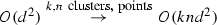
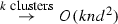
• $O(ik(d^3 + nd^2))$

The best run-time EM-T can have is O(knd) for the E-Step and O(knd) for the M-Step. This yields O(inkd). The EM-T algorithm takes as input data $\mathrm {\Delta }$, the number of blocks k and a convergence threshold $\epsilon$ and produces a set of Gaussian distributions $G_1, G_2, \ldots , G_k$. Each Gaussian has a set of parameters. For every ${\mathbf {x}} \in \mathrm {\Delta }$, there is a Gaussian where ${\mathbf {x}}$ is most likely from. The algorithm iteratively alternates between (1) computing log$\text {-}$likelihood of each data point belonging to each Gaussian (E-step) (2) recalculating the parameters (M-step). Iteration continues until the set of means is stable.

To make discussion easier, we assume at each ith iteration, $G^i_j$ is the jth Gaussian in the set ${\mathsf {G}}^i$. Lastly, we presume a Gaussian is a set of parameters $(\mu .\mathrm {\Sigma },\Pr (G),w_{{\mathbf {x}}},X)$ where $\mu$ is the mean, $\mathrm {\Sigma }$ the covariance matrix, $\Pr (G)$ the prior, $w_{{\mathbf {x}}} \in {\mathbb {R}}$ the likelihood and $X\subseteq \mathrm {\Delta }$. Line 6, the initialization of the starting set of Gaussians, greatly affects EM-T’s performance, since it is a greedy algorithm. Most spaces will be non-convex, so local optima will “trap” the Gaussians. The assignment phase, Lines 10–16, maps each data point to Gaussians with likelihoods. Originally $k,m\ll |\mathrm {\Delta }|$; consequently, the algorithm is often said to be linear in the size of data, i.e., $O(|\mathrm {\Delta }|)$. A number of details are unspecified in the EM-T. One of the most significant is what do if the covariance matrix becomes singular. Since a Gaussian might become empty, the number of blocks can differ from the original k. Further, points can be equally near more than one Gaussian; therefore, ties must be broken.

The remainder of this paper is as follows. Section 3 algorithmically explains $\hbox {EM}^*$ and provides some theoretical insights. Section 4 presents results from our experiment as well as comparison with EM-T. Section 5 is the summary and conclusions from our work.

3 $\hbox {EM*}$: EM clustering algorithm for big data

We observe that both (1) continually revisiting data and (2) visiting all data are two of the most prominent problems for EM-T. We embed EM-T into a nonlinear hierarchical data structure (max heap) that allows us to (1) separate data that needs to be revisited from data that does not and (2) narrow the iteration toward the data that is more difficult to cluster. We call this extension of EM-T algorithm $\hbox {EM*}$. A notational outline of $\hbox {EM*}$ is presented in Alg. 2.

In our algorithm, initialization of the parameters is identical to EM-T. In the E-step phase, each piece of active data is compared to each Gaussian distribution and assigned to the most likely one. In the M-step phase, each Gaussian distribution is altered to better represent the data assigned to it during the previous phase, and the data is processed to determine which pieces are still active.

We introduce a concept of active data as a means of differentiating between the data that needs to be revisited on a subsequent iteration from the data that does not. On the first iteration, every piece of data is marked as active. During the E-step phase, when a piece of data is assigned to a Gaussian, it is placed in a heap structure for that Gaussian (mutual exclusion blocks are implemented for data protection across the heaps). The values in the heap are representative of the likelihood used for data and Gaussian. Data that is higher in the heap indicates that it is more likely to be from the Gaussian; data that is lower in the heap indicates it is less likely—perhaps even unlikely—from the Gaussian. In the M-step phase, each Gaussian is updated as EM-T is, by taking into consideration all the data points assigned to that Gaussian. The heap for that Gaussian then used to determine which pieces of data are marked as active.

The heap for a particular Gaussian represents a partial ordering (the path from the root to any leaf) over the data assigned to that Gaussian. This offers a natural view of the relative importance of the data. Data residing in leaf nodes is most important and is re-clustered in the following iteration. Data that is high in a Gaussian’s heap is considered closely bound to that Gaussian and unlikely to change; consequently, it is ignored in the following iteration. Determining the optimal break that separates the two yielded our first heuristic described presently, but we imagine there exist different (and perhaps better depending on context) breaks. We do not use “hyperplanes,” even in its broadest sense, since level-wise, the partial order can be violated, but there may be some notion that could become useful. Following the Gaussian update and data culling in this phase, new likelihoods are calculated for the data remaining in the heap with the partial ordering being restored where it may have broken. Our implementation terminates once $99\%$ of the data in the leaf nodes remains unchanged in subsequent iterations and it is discussed in “Experiments” section.

3.1 Run time for EM*

EM*, in contrast to EM-T, has, at each iteration i, $n \leftarrow O(\lceil n/2 \rceil )$ and each subsequent iteration takes half as long, $i \leftarrow i/2$. We know from basic complexity theory that $cO(n) = O(n)$ for some positive integer c and would rightfully argue it does not matter. From a practical standpoint of big data, however, this makes an effective and dramatic difference evidenced by our experimentation. In many instances, EM-T simply could not converge. Let $l=\lceil n/2\rceil$ and $t=\lfloor n/2\rfloor$ denote the number of data points located in the leaf nodes and not located in the leaf nodes. The general and best run time of EM* is $O(i_2k(d^3 +nd^2)+li_2 \log n)$ and $O(i_2knd + li_2\log t)$, respectively ($i_2 \ll i$). Logarithmic parts come from heap updates.

4 Experiments and results

To determine how well our $\hbox {EM*}$ algorithm performs, we compared it against the EM-T algorithm. Both algorithms were run against both real-world and synthetic data sets. We implemented $\hbox {EM*}$ and EM-T in a way that would allow them to partition data for an arbitrary number of blocks. If the true clusters are known, for a given arbitrary number of blocks, final clusters are determined by measuring the Euclidean (this is the most popular choice) distances between true cluster centers and predicted cluster centers.

The $\hbox {EM*}$ algorithm stops when 99%, $\epsilon \le 0.01$, of the data points in the leaf nodes between consecutive iterations are the same. This criterion guarantees not only stability of the heaps but also completion of clustering task. In other words, our algorithm converges using the structure as distinct from EM-T. 99% threshold is heuristically chosen. During the experiments, we observed that our stopping criterion is less sensitive than $\epsilon$ used in EM-T. Increasing and decreasing the threshold does not affect it that much since our algorithm benefits from the structure to converge. Average size of the heap managed by the EM* algorithm at each iteration is n / k. In this paper, we are not: (1) improving EM through initialization and (2) presuming the number of blocks affects the results.

All experiments were performed on an 4-core Intel Core i7 with 16GB of main memory running 64-bit OS X El Capitan. Both algorithms are implemented using Python 2.7.10, and multivariate data generator (mixture of Gaussians) is in R 3.2.4.

4.1 Experiments with real-world data sets

4.1.1 Breast cancer data set

In the first experiment, we tested our $\hbox {EM*}$ algorithm over the well-known Wisconsin breast cancer data set [41]. This modest size data set is a good starting point for our comparison, since neither the size nor dimensions would be considered big. This data set consists of 699 tuples and 11 variables and is publicly available in the UCI Machine Learning Repository [42]. The feature set describes multiple histopathologies of resected breast tissue as whole numbers in [1,10]. After missing records (minor, insignificant number), $\hbox {EM*}$ and EM-T algorithms were run over the data set, size of 683 $\times$ 9, to cluster benign and malignant tumors. The original clusters have 444 and 239 data points, and thus, the baseline cluster error was 0.35.

We ran both algorithms against different number of clusters and used different $\epsilon$ values for EM-T, but we only give the results for $\epsilon \le 0.0001$ . We note that EM-T was unable to convergence for $\epsilon \le 0.01$ in 10K iterations. Figure 1 demonstrates the experimental results for training time in seconds, number of iterations and accuracy. Results show that $\hbox {EM*}$ was able to drastically reduce training time of EM-T. Performance of both algorithms in terms of cluster error was similar. Accuracy values for $\hbox {EM*}$ and EM-T were between 88–96 and 87–97%, respectively. However, $\hbox {EM*}$ performs better than EM-T for the true number of clusters. Algorithms were also ran against larger number of clusters, and we observed that $\hbox {EM*}$ makes EM-T more efficient for large number of clustering problems.

4.1.2 US census data set

Census income data set consists of approximately 50 K data points and 14 features, 6 continuous and 8 discrete, and is publicly available in the UCI Machine Learning Repository. At the preprocessing step, we removed the missing information and column-wise normalized the data. The clean data set had 45 K data points in 6 (only continuous attributes) dimensions. In this experiment, clustering task is to separate people who make over 50 K from who do not.

Figure 2 shows the experimental results. EM-T ran for 1K and 10K iterations with $\epsilon \le 0.01$ and was only able to converge for $k =2$. We observed that $\hbox {EM*}$ was effective at reducing training time of EM-T and performs better for large number of clustering problems once again. We note that the $\epsilon$ value used for EM-T is way larger than the $\epsilon$ values commonly recommended. Thus, $\hbox {EM*}$ reduces training time of EM -T much more for smaller $\epsilon$ values.

Fig. 1

Comparison of EM-T and $\hbox {EM*}$ over breast cancer data set and it provides a numerical complexity analysis for EM-T and $\hbox {EM*}$. Note that EM-T did not converge during maximum number of iterations

Fig. 2

Comparison of EM-T and $\hbox {EM*}$ over census income data set and it provides a numerical complexity analysis for EM-T and $\hbox {EM*}$. Note that EM-T did not converge during maximum number of iterations

4.2 Experiments with synthetic data sets

4.2.1 Galactic survey data set

This data set is a catalog of stars and was generated using the TRILEGAL 1.6 star count simulation [3, 43, 44]. Galactic survey data set consists of 910K stars and is available at http://www.computationalastronomy.com [43]. In this experiment, our clustering goal is to efficiently recover the three major components that make up our home Galaxy: the halo, thick disk and thin disk. 49, 30 and 21% of the date points belong to halo, thin disk and thick disk, respectively. Experiments were shown that mass ratio, effective temperature, surface gravity and distance modulus are the features that reveal characteristics of this data to separate the galactic components [3]. Thus, we ran EM* over these four attributes.

Figure 3 shows the experimental result for EM-T and $\hbox {EM*}$ over Galaxy Survey Data Set. $\hbox {EM*}$ drastically reduced training time of EM-T. Since training time of EM-T takes around 7.5 h, we did not run it for $k=200$. We do not give the accuracy figures because both algorithms performed similar. $\hbox {EM*}$ for $k =200$ was around 1.7 h faster than EM-T for $k =100$.

Fig. 3

Results for EM-T and $\hbox {EM*}$ over galactic survey data set. EM-T did not converge during maximum number of iterations

4.2.2 Multivariate synthetic data sets

We generated large multivariate data sets, mixtures of Gaussians, to observe performance of $\hbox {EM*}$. Experiments are designed over high-dimensional data, large number of clusters and data points. We repeated each experiment five times and averaged the results while observing effect of dimensionality and cluster numbers. Scalability experiments were not repeated due to time constraints. Covariances are randomly selected from [0.01, 0.04] and variances are assigned, the smallest being 0.1 and the proportion of the largest one to the smallest being 10. Centers of the clusters are assigned as the first one being d-dimensional vector of ones, the second one being d-dimensional vector of threes and so on. Figure 4 represents an example of three mixture of Gaussian distributions on two variables generated with those parameters. Maximum number of iteration for a run was a 1K, the stopping criterion $\epsilon$ was 0.01, and each of the true clusters had the same amount of the data points.

Our first experiment was designed to test scalability of $\hbox {EM*}$. We observed how $\hbox {EM*}$ and EM-T perform over large data sets where $n=\{1.5,3,4.5,6,7.5,9, 10.5\}$ millions data points while $k =20$ and $d=20$. EM-T, according to the literature, is capable of handling high-dimensional data sets. Second, we examined the performance of $\hbox {EM*}$ over high-dimensional data sets where $d=\{20,40,60,60,80,100,150,200,250,300,400,450\}$ while $n=45\hbox {K}$ and $k =10$. Lastly, we generated 45 K data points, each cluster having 15 K points, in 10 dimensions and tested our heap-based algorithm over large number of clusters where $k =\{10,20,30,40,50,60,70,80,90,100\}$.

Figure 5 shows experimental results for $\hbox {EM*}$ and EM-T over multivariate data sets. EM-T and $\hbox {EM*}$ clustered all data points correctly at each experiment; thus we only scrutinize execution time and number of iterations. $\hbox {EM*}$ always outperforms EM-T in run time. One striking observation is the improved efficiency when number of clusters is large. $\hbox {EM*}$ drastically reduced training time when compared to EM-T for large number of clusters. $\hbox {EM*}$ converged approximately around 11–13 iterations while increasing number of clusters, whereas EM-T was not able to converge in 1K iterations after 30 clusters. EM-T was only able to converge 2 out of 5 data sets for $k =30$. Execution time and iteration counts are given in Fig. 5.

Unsurprisingly, as we increase dimensionality, both EM-T and $\hbox {EM*}$ converge at the same number of iterations and execution time. Presumably, the curse of dimensionality, with its effects on distance, reduces any advantage $\hbox {EM*}$ possesses.

Fig. 4

How the synthetic data sets are generated. Mixture of three Gaussian distributions. Each distribution has 300 K data points on two dimensions

Fig. 5

Comparison of EM-T and EM* over large synthetic data sets. Performance of EM-T and EM* varying size, dimensionality and number of clusters. Note that EM-T did not converge during maximum number of iterations while k is increased

4.3 Observing data in the heap: good and bad data

Our goal was to dichotomize the data as good and bad using the heap structure to make iterative learning algorithms computationally more efficient. Our initial approach was to empirically determine this break with the intuition that the bound was location near or at the median. By fixing the median in the heap, and subsequently locating bad data points in the heap, we confirmed that that bad data points reside in the leaves.

Fig. 6

Plots of likelihood of median being on each node in the heap. The plots were made with R and ggplot2. The blue lines denote loess smoothers (color figure online)

Fig. 7

Plots of node-wise distribution of bad data points in the heap while changing amount of the bad data in the data. The plots were made with R and ggplot2. The histogram coloring is from R’s default coloring scheme (color figure online)

4.3.1 A simple heuristic: median

In effectively producing a heuristic that separates good from bad, we wanted our heuristic to be driven by the data. We began motivated by the principle that most of the bad data resides in the leaves and that the median is as good as other measures, but we also wanted a heuristic that was computationally cheap to find. What we provide here are our results in identifying the median in a heap mixed with both good and bad data. Our results support our conjecture. An interesting observation is that we are unaware of any systematic data science approach to examining this kind of heap property and suggest fertile areas of exploration with regard to statistical analysis.

4.3.2 Observing median in the heap

We randomly generated six data sets of sizes $n=\{27, 51, 101, 231, 351, 495 \}$. The data points are randomly picked numbers between [1, 100000] without replacement. We then built 2M heaps for each data set by sampling each data set without replacement 2M times to observe location of median in the heap. Figure 6 demonstrates the likelihood of median being on each node in the heap. As seen from the plots, the node that has the highest likelihood for median is left most node above the leaf nodes all the time. We also observed level-wise location of median in the heap. To keep the discussion simple, we do not show the figures demonstrating median location level-wise in the heap. However, results show median locates in the last two levels of the heap. Since this is not a good bound, we located bad data points in the heap for the next step to decide a better bound.

4.3.3 Distribution of bad data in the heap

We experimentally generated both bad and good data (larger and smaller mean square error) and inserted them into the heap. First, good data and bad data were generated randomly with replacement. Second, 1M heaps were built randomly without replacement. Third, the location of the bad data points was detected. Figure 7 shows node-wise bad data distribution for randomly generated 200 points, and Fig. 8 demonstrates how the amount of bad data in the leaf nodes changes, while increasing the amount of the bad data in the data. This experiment was carried out while 1, 10, 20, 30,40, and 50% of the data was bad in the data. The results demonstrate that when 1% of the data is bad, all the bad data points are located in the leaf nodes. Other experiments show that while 10, 20, 30, 40, 50% of the data is bad, 99, 98, 94, 90 and 84% of the bad data points are in the leaf nodes, respectively. This experiment is also done for different number of data points. The results were similar. In conclusion, the heap is an efficient structure for separating both good and bad data.

4.4 Convergence threshold $\epsilon$, KL distance and entropy

To understand why EM* performs better than EM-T, we observed:

• Convergence threshold $\epsilon$

• Entropy distribution among clusters

• The total entropy for W, which represents the likelihood matrix for clusters and data points

• The Kullback–Leibler (KL) distance for each cluster between consecutive iterations.

Informally, KL distance measures the difference between two probability distributions, using one as a starting point (thus, KL is not a metric because it is not symmetric). Since the underlying distribution of clusters is multivariate normal, the KL distance for each cluster between consecutive iterations was calculated using formula (1). After calculating the KL distance for each cluster, we added the distances and formulated the result as a measure of difference between consecutive iterations. To address the lack of symmetry in KL, we calculated $\mathrm{KL}1 = \mathrm{KL}(G^i_j || G^{i+1}_j)$ and $\mathrm{KL}2 = \mathrm{KL}(G^{i+1}_j || G^i_j)$. We also calculated the total entropy and cluster-wise entropy distribution at each iteration.

$$\begin{aligned}&A = tr\left( G^{i+1}_j.\mathrm {\Sigma }^{-1}G^i_j.\mathrm {\Sigma }\right) \nonumber \\&B =\left( G^{i+1}_j.\mu - G^i_j.\mu \right) ^T G^{i+1}_j.\mathrm {\Sigma }^{-1}\left( G^{i+1}_j.\mu - G^i_j.\mu \right) \nonumber \\&C = \log \left( {\mathrm {det}} G^i_j.\mathrm {\Sigma }/{\mathrm {det}} G^{i+1}_j.\mathrm {\Sigma }\right) - d\nonumber \\&\mathrm{KL} \left( G^i_j || G^{i+1}_j\right) = 1/2[A + B - C] \end{aligned}$$

(1)

We observed those measures over different synthetic and real-world data sets and obtained similar results. We only show experimental results for the breast cancer data set and the multivariate normal synthetic data set used to test performance of the two algorithms over different number of clusters. Additional figures are omitted for brevity. Regarding the experiments involving the breast cancer data set, Figs. 9 and 10 demonstrate the experimental results for EM* and EM-T parameterized with 5 clusters and $\epsilon = 0.01$. We note that EM-T did not convergence during maximum number of iterations. Figures 11 and 12 represent the results for the multivariate normal data set. We note that EM-T and $\hbox {EM*}$ convergence in 89 and 8 iterations, respectively, for $\epsilon = 0.01$. The experiments over breast cancer data set include the case where EM-T fails to converge, and the experiments over the multivariate data represent the case where the both algorithms convergence during the maximum number of iterations.

Fig. 8

Plot of percentage of bad data in the leaf nodes while increasing amount of the bad data in the data. The plots were made with R

Fig. 9

Plots of change in total entropy and entropy distribution among clusters over breast cancer data set. Note the difference in scale of the plots resulting from EM-T’s failure to converge within the maximum number of iterations. The blue lines denote loess smoothers (color figure online)

Fig. 10

Plots of change in convergence threshold $\epsilon$ and KL distance over breast cancer data set. Note the difference in scale of the plots resulting from EM-T’s failure to converge within the maximum number of iterations. The blue lines denote loess smoothers (color figure online)

Fig. 11

Plots of change in total entropy and entropy distribution among clusters over the synthetic multivariate normal data set. The blue lines denote loess smoothers (color figure online)

Fig. 12

Plots of change in convergence threshold $\epsilon$ and KL distance over the synthetic multivariate normal data set. The blue lines denote loess smoothers

Results reveal that $\hbox {EM*}$ always appears to make better decisions than EM-T while finding the true parameters. During its execution, the $\epsilon$ value almost monotonically decreases. In comparison, EM-T’s parameter update process does not appear monotonic over the breast cancer data. However, both algorithms have similar trends over the synthetic data set for $\epsilon$. We observe similar trends in the figures portraying the KL distance, total entropy and cluster-wise entropy distribution. Figures 11 and 12 demonstrate that EM-T and EM* show similar trends over the synthetic data set, but the only difference is that $\hbox {EM*}$ converges faster than EM-T.

These results support our initial intuition that when clustering a large data set, a significant portion of the data will not change clusters or will do so only a limited number of times. Introducing heap data structures to EM-T has allowed us to develop an algorithm that significantly lessens the amount of data considered on each iteration of the algorithm, effectively reducing the training run time complexity. Further, the optimization occurs now over a structure and inspection of where data exists, rather than from an objective function. Of the interesting questions that this raises, what is the class of structures themselves that allow for this optimization? What is the best (efficiency, accuracy, etc.) structure? Can we effectively share the goodness or badness of data globally?

5 Summary and conclusions

We have presented an extension to the traditional EM called EM* that drastically reduced time complexity of EM algorithm over large real-world and synthetic data sets. We achieved this introducing a max heap over traditional EM algorithm ordering data by its likelihood that (1) separates data that needs to be revisited from data that does not and (2) narrows the iteration to focus on data that is more difficult to cluster. We believe, in general, hierarchical management of data in iterative optimization algorithms like EM presents an effective strategy to deal with scaling data and have begun employing this technique on different learning algorithms. We are further examining other algorithms, parallelizing and distributing the heap. Lastly, we are employing EM* to larger data sets and studying the results. Lastly, we have submitted work on the theoretical underpinnings of this approach, both addressing this instance, and to iterative optimization problems of this ilk in general.

References

Kurban, H., Jenne, M., Dalkilic, M.M.: EM*: an EM algorithm for Big Data. In: 2016 IEEE International Conference on Data Science and Advanced Analytics (DSAA), pp. 312–320 (2016)
Wu, X., Kumar, V., et al.: Top 10 algorithms in data mining. Knowl. Inf. Syst. 14(1), 1–37 (2007)
Jenne, M., Boberg, O., Kurban, H., Dalkilic, M.M.: Studying the milky way galaxy using ParaHeap-k. IEEE Comput. Soc. 47(9), 26–33 (2014)
Arthur, D., Vassilvitskii, S.: “k-means++,” The advantages of careful seeding. In: Proceedings of the Eighteenth Annual ACM-SIAM Symposium on Discrete Algorithms, pp. 1027–1035 (2007)
Bahmani, B., Moseley, B., Vattani, A., Kumar, R., Vassilvitskii, S.: Scalable k-means++. Proc. VLDB Endow. 5(7), 622–633 (2012)
Dempster, A.P., Laird, N.M., Rubin, D.B.: Maximum likelihood estimation from incomplete data via the em algorithm. J. R. Stat. Soc. 39(1), 1–38 (1977)
Wu, C.F.J.: On the convergence properties of the EM algorithm. Ann. Stat. 11(1), 95–103 (1983)
Yuille, A.L., Stolorz, P., Utans, J.: Mixtures of distributions and the EMalgorithm. Neural Comput. 6(1), 334–340 (1994)
Xu, L., Jordan, M.: On convergence properties of the EM algorithm for Gaussian mixtures. Neural Comput. 8(1), 129–151 (1996)
Roweis, S., Ghahramani, Z.: A unifying review of linear Gaussian models. Neural Comput. 11(2), 305–345 (1999)
Ghosh, A.K., Chakraborty, A.: Use of EM algorithm for data reduction under sparsity assumption. Comput. Stat. 32(2), 387–407 (2017)
McLachlan, G.J., Krishnan, T.: The EM Algorithm and Extensions. Wiley, New York (2007)
Jung, Y.G., Kang, M.S.: Clustering performance comparison using K-means and expectation maximization algorithms. Biotechnol. Biotechnol. Equip. 28(1), 44–48 (2014)
Do, C.B., Batzoglou, S.: What is the expectation maximization algorithm. Nat. Biotechnol. 26, 897–899 (2008)
Watanabe, M., Yamaguchi, K.: The EM Algorithm and Related Statistical Models. CRC Press, Boca Raton (2003)
Hastie, T., Tibshiraniet, R., Friedman, J.: The EM algorithm an old folk-song sung to a fast new tune. J. R. Stat. Soc. Ser. B 59(3), 511–567 (1997)
Zhang, Y., Brady, M., Smith, S.: Segmentation of brain MR images through a hidden Markov random field model and the expectation-maximization algorithm. IEEE Trans. Med. Imaging 20(1), 45–57 (2001)
Langari, R., Wang, L., Yen, J.: Radial basis function networks, regression weights, and the expectation–maximization algorithm. IEEE Trans. Syst. Man Cybern. Part A 7(5), 613–623 (1993)
Dayan, P., Hinton, G.E.: Using expectation–maximization for reinforcement learning. Neural Comput. 9(2), 271–278 (1997)
Tang, M., et al.: On improved EM algorithm and confidence interval construction for incomplete \({\rm r}\times {\rm c}\) tables. Comput. Stat. Data Anal. 51(6), 2919–2933 (2007)
Lindstrom, M.J., Bates, D.M.: Newton-Raphson and the EM algorithm for linear mixed-effects models for repeated-measures data. J. Am. Stat. Assoc. 83, 1014–1022 (1988)
Epperson, J.F.: An Introduction to Numerical Methods and Analysis. Wiley, New York (2013)
Jamshidian, M., Jennrich, R.I.: Conjugate gradient acceleration of the EM algorithm. J. Am. Stat. Assoc. 88, 221–228 (1993)
Jamshidian, M., Jennrich, R.I.: Acceleration of the EM algorithm by using quasi-Newton methods. J. R. Stat. Soc. 59, 569–587 (1997)
Neal, R. M., Hinton, G. E.: A view of the EM algorithm that justifies incremental, sparse, and other variants. In: Jordan, M.I. (ed.) Learning in Graphical Models, pp. 355–368. MIT Press, Cambridge (1999)
Booth, J.G., Hobert, J.P.: Maximizing generalized linear mixed model likelihoods with an automated Monte Carlo EM algorithm. J. R. Stat. Soc. Ser. B (Methodol.) 61(1), 265–285 (1999)
Meng, X.L., Rubin, D.B.: Maximum likelihood estimation via the ECM algorithm: a general framework. Biometrika 80(2), 267–278 (1993)
Liu, C., et al.: The ECME algorithm: a simple extension of EM and ECM with faster monotone convergence. Biometrika 81(4), 633–648 (1994)
Celeux, G., Chauveau, D., Diebolt, J.: On stochastic versions of the EM algorithm. Doctoral dissertation, INRIA (1995)
Wei, G.C., et al.: A Monte Carlo implementation of the EM algorithm and the poor mans data augmentation algorithms. J. Am. Stat. Assoc. 85(411), 699–704 (1990)
Liu, C., et al.: Parameter expansion to accelerate EM: the PX-EM algorithm. Biometrika 85(4), 755–770 (1998)
Liu, J.S., Wu, Y.N.: Parameter expansion for data augmentation. J. Am. Stat. Assoc. 94(448), 1264–1274 (1999)
Tanner, M.A., Wong, W.H.: The calculation of posterior distributions by data augmentation. J. Am. Stat. Assoc. 82(398), 528–550 (1987)
Lange, K.: A quasi-Newton acceleration of the EM algorithm. Stat. Sin. 5(1), 1–18 (1995)
Louis, T.A.: Finding the observed information matrix when using the EM algorithm. J. R. Stat. Assoc. Ser. B 44, 226–233 (1982)
Efron, B., Hinkley, D.V.: Assessing the accuracy of the maximum likelihood estimator: observed versus expected Fisher information. Biometrika 51(6), 457–482 (1978)
Bradley, P., Fayyad, U., Reina, C.: Scaling EM clustering to large databases. Technical report, Microsoft Research (1997)
Bradley, P., Fayyad, U., Reina, C.: Scaling clustering algorithms to large databases. In: ACM KDD Conference (1998)
Fanstrom, F., Lewis, J., Elkan, C.: Scalability for clustering algorithms revisited. SIGKDD Explor. 2(1), 51–57 (2000)
Ordonez, C., Omiecinski, E.: FREM: fast and robust EM clustering for large data sets. In: ACM CIKM Conference, pp. 590–599 (2002)
Mangasarian, O.L., Wolberg, W.H.: Cancer diagnosis via linear programming. SIAM News 23(5), 1–18 (1990)
Bache, K., Lichman, M.: UCI Machine Learning Repository. http://archive.ics.uci.edu/ml (2013)
Jenne, M., Boberg, O., Kurban, H., Dalkilic, M. M.: Computational astronomy. http://www.computationalastronomy.com (2014)
Girardi, L., Groenewegen, M.A.T., Hatziminaoglou, E., Costa, L.: Star counts in the galaxy. Simulating from very deep to very shallow photometric surveys with the trilegal code. Astronomy Astrophys. 4(36), 895–915 (2005)
Acknowledgements
The authors thank the editor and anonymous reviewers for their informative comments and suggestions. This work was partially supported by NCI Grant 1R01CA213466-01.
Author information
Authors and Affiliations
Corresponding author
Ethics declarations
Conflict of interest
On behalf of all authors, the corresponding author states that there is no conflict of interest.
Additional information
This paper is an extension version of the DSAA’ 2016 paper “EM*: An EM algorithm for Big Data” [1].
Rights and permissions
About this article
Cite this article
Kurban, H., Jenne, M. & Dalkilic, M.M. Using data to build a better EM: EM* for big data. Int J Data Sci Anal 4, 83–97 (2017). https://doi.org/10.1007/s41060-017-0062-1
Received:
Accepted:
Published:
Issue Date:
DOI: https://doi.org/10.1007/s41060-017-0062-1