Importance of the Geocoding Level for Historical Demographic Analyses: A Case Study of Rural Parishes in Sweden, 1850–1914

Abstract

Geocoding longitudinal and individual-level historical demographic databases enables novel analyses of how micro-level geographic factors affected demographic outcomes over long periods. However, such detailed geocoding involves high costs. Additionally, the high spatial resolution cannot be properly utilized if inappropriate methods are used to quantify the geographic factors. We assess how different geocoding levels and methods used to define geographic variables affects the outcome of detailed spatial and historical demographic analyses. Using a longitudinal and individual-level demographic database geocoded at the property unit level, we analyse the effects of population density and proximity to wetlands on all-cause mortality for individuals who lived in five Swedish parishes, 1850–1914. We compare the results from analyses on three detailed geocoding levels using two common quantification methods for each geographic variable. Together with the method selected for quantifying the geographic factors, even small differences in positional accuracy (20–50 m) between the property units and slightly coarser geographic levels heavily affected the results of the demographic analyses. The results also show the importance of accounting for geographic changes over time. Finally, proximity to wetlands and population density affected the mortality of women and children, respectively. However, all possible determinants of mortality were not evaluated in the analyses. In conclusion, for rural historical areas, geocoding to property units is likely necessary for fine-scale analyses at distances within a few hundred metres. We must also carefully consider the quantification methods that are the most logical for the geographic context and the type of analyses.

1 Introduction

This study analyses the methodological issues related to including a micro-level geographic context in longitudinal demographic analyses. Within demographic and epidemiological studies, an expanding field of research has focused on spatial aspects at both the micro-level (individual level) and the macro-level (aggregated level) (cf. Voss 2007; Logan 2012). In addition, these analyses are often longitudinal; therefore, they cover longer time periods and follow individuals throughout their life courses. Such analyses are common in modern studies but less so in historical studies. Within the field of historical demography, several scholars have included the geographic context on a macro-level, meaning that they have analysed the influence of geographic factors operating on a coarse scale, such as villages and parishes, on the aggregated historical populations (e.g., DeBats 2011; Gutmann et al. 2005; Gregory 2008; Kasakoff et al. 2013). Studies that analyse micro-level geographic factors are also becoming more common (e.g., Ekamper 2010), although they are seldom longitudinal because there are few historical longitudinal demographic databases that geocode individuals to a more precise location, such as the property unit/parcel boundary or building, over long time periods. Recently, however, certain longitudinal demographic databases have been geocoded on a detailed level (e.g., Villarreal et al. 2014; Hedefalk et al. 2015, 2017b), which enables the inclusion of micro-level geographic context in longitudinal historical analyses. In this study, we use the geocoded Scanian Economic Demographic Database (SEDD) to perform our analyses for the period from 1850 to 1914 (Hedefalk et al. 2017b).

Geographic context is a broad term that includes all of the geographic factors that affect the associated individuals. Such factors are important for historical mortality studies. For example, the micro-level geographic factors of population density, soil conditions (via their effect on agricultural productivity), and proximity to communication networks, wetlands (natural habitats of malaria-carrying mosquitoes), health centres and hospitals potentially had an effect on mortality in historical societies (Claësson 2009; Lazuka et al. 2016; Hedefalk et al. 2017a). To analyse the effect of these geographic context factors, appropriate quantification methods are required. The quantified geographic context factors throughout this paper are denoted as geographic context variables.

Historical studies using macro-level or micro-level geographic context factors have contributed to the understanding of how demographic outcomes are affected by the environment. The recent and ongoing geocoding of databases on the micro-level can be used to account for the variation of context variables on a more local scale. The inclusion of such micro-level geographic context variables in longitudinal analyses of historical populations requires historical sources, such as detailed maps, to enable the geocoding of demographic databases. In general, such geocoding contains two costly processes. The first process collects and prepares the historical geographic data necessary for geocoding. The second process links individuals to historical geographic objects at the micro-level (e.g., urban blocks, property units or buildings). Efficient methods are required to perform both of these processes (cf. e.g., Hedefalk et al. 2015). An important issue in this context is to determine the geographic level at which the geocoding should be performed. The general rule is that the more detailed the geocoding, the more expensive the process becomes. For example, the geocoding of individuals at the building level is likely more costly than that at the property unit level. For longitudinal data, one must also consider the residential histories and include geographic changes that might affect both the geocoding and the geographic factors. Hence, performing geocoding on a highly detailed level for long time periods and accounting for changes in geography involve high costs. Finding an optimal geocoding level that balances cost and applicability requires an understanding of the scale at which the geographic factors operate. Moreover, the most logical quantification methods for certain types of analyses must be determined. Otherwise, the high spatial resolution of the geocoding cannot be properly utilized and the demographic models might produce unreliable results.

However, the appropriateness of the geocoding level, both in the spatial and temporal aspect (accounting for geographical changes), and the appropriateness of the quantification of geographic context variables have received little attention in historical demographic research. Nevertheless, several studies have focused on the geocoding quality of modern demographical and epidemiological data (Zandbergen 2007, 2009; Griffith et al. 2007; Mazumdar et al. 2008; Vieira et al. 2010), although such information is seldom considered in studies that apply demographic and spatial analyses. In historical demography this problem might be even more pervasive because of the later adoption of spatial analysis in this field.

Thus, this study contributes to the literature by offering insights into the importance of using appropriate quantification methods and choosing the geographic level so that the most suitable geocoding is used for longitudinal demographic analyses on the micro-level. The overall aim is to study is how the geographic level of the geocoding and the choice of quantification methods for the geographic context affect the results of historical demographic analyses. The novelty of this study is the use of longitudinal and micro-level demographic and geographic data. Previous studies on the effect of geocoding level have mostly used data that cover a short period that does not encompass substantial geographic changes. Hence, in this study, we are also able to analyse how different temporal models (i.e., if and how temporal geographic changes are modelled) affect the results of the demographic analyses.

Our analysis is conducted in the context of mortality in five rural parishes in Sweden during the nineteenth century. We use individual-level longitudinal data from the Scanian Economic Demographic Database (SEDD) (Bengtsson et al. 2014), which has recently been geocoded (Hedefalk et al. 2015, 2017b). In this geocoding, approximately 53,000 individuals have been linked to the property units¹ at which they lived. The SEDD database has been frequently used in historical demographic studies, and after controlling for socio-economic factors, large regional differences have been observed in both childhood and adult mortality (among other differences) until the twentieth century (Bengtsson and Dribe 2010, 2011). The reason for these regional differences is partly unknown. One hypothesis is that the geographic factors related to infectious disease exposure could be responsible for such differences in mortality. Therefore, we selected two geographic context variables that are related to exposure to infectious diseases: population density and proximity to wetlands. The latter is considered a possible indicator of exposure to malaria, which was a problem in this area during the nineteenth century (Lindgren and Jaenson 2006). Although the results of the mortality analyses themselves might offer insights into how the geographic context affected mortality in the study area, the main purpose is not to conduct a complete analysis of mortality. Therefore, all possible determinants of mortality are not evaluated for the study area. In addition to including a more extensive historical analysis, a complete analysis of mortality should include other geographic context variables that could potentially influence mortality.

This paper is organized as follows. Section 2 reviews related studies on the geocoding of demographic databases and the impact of geographical context in demographic analyses. Section 3 describes the data and methodology used in this study. The main focus in this work is the geographic levels of the geocoding and the definitions of the geographic context variables. The results are reported in Sect. 4, and the paper concludes with a discussion and the conclusions in Sect. 5.

2 Related Studies

2.1 Geocoding of Demographic Databases

Geocoding is the process of assigning address information to a coordinate pair, a polygon or another type of geographical unit. Through this process, individuals can be linked through the address information to one or multiple physical locations in the geographical reference data. The geocoding process differs depending on whether the data are modern or historical and whether they are static or dynamic.

Assigning individuals to detailed physical locations is relatively straightforward when conducting modern studies in which adequate records are available to assign individuals to standardised addresses that in turn can be linked to modern reference data (nevertheless, such a process is not free from quality problems (cf. Zandbergen 2009). Depending on the address information and the reference data, the geocoding can be applied to a wide range of geographical levels, such as counties, cities, census blocks, street segments, property units/parcel boundaries, buildings and even apartments. For historical data, standardised addresses are seldom available and geographic reference data (e.g., historical maps) to which the addresses can be linked are scarce. Therefore, in most cases, the physical locations of the individuals are recorded on rather coarse administrative levels (e.g., parishes or villages in which they lived). To enable geocoding on a detailed level, tailored geographic reference data often must be created. A common method of creating such reference data is to scan, georeference and digitize historical maps that contain sufficient geometric and address information that can be used in the geocoding process (cf. Hedefalk et al. 2015).

Geocoding of longitudinal demographic data also requires that the geographic reference data are longitudinal; thus, all of the changes in the geographic objects to which the individuals are linked and when these changes occurred must be known. Typical examples of such changes are the emergence of new property units or smaller changes in the borders of the existing property units. The geometrical changes in the reference data can be represented with an object-lifeline model. This model shows when a geographic object was created, when and how it was changed, and when it ceased to exist (Worboys and Duckham 2004). In addition, the modelling should include the geometrical changes of other geographic objects (e.g., wetlands) that are altered through time and included in the definition of the geographic context variables (e.g., proximity to wetlands).

To create such object-lifeline representations are not always possible because the historical sources of the geography (mainly historical maps) are not always available or sufficiently frequent in time to cover all of the geographic changes (because they are only snapshots in time). Additionally, even if historical sources are available (e.g., cadastral dossiers that describe the changes in property units), it is cumbersome to collect and digitize such information.

However, in recent years, selected studies have linked longitudinal historical populations to a more detailed physical level. Villarreal et al. (2014) studied the historical health and environmental conditions in seven major U.S. cities from 1830 to 1930 and developed the Historical Urban Ecological data set (HUE), which contains digitized crime, disease, demographic, property, land and tax information from annual municipal reports at the ward level. By including accurate digital representations of historical city street centrelines, these authors created the tools necessary to link the ward-level dataset to city blocks. Moreover, Hedefalk et al. (2015) geocoded approximately 53,000 individuals to their rural property units in the SEDD database for the time period 1813–1914. Two main challenges arose in this geocoding process. The first challenge was to create longitudinal object-lifelines of the property units based on historical maps and supplementary textual sources, such as poll tax registers and cadastral dossiers. The second challenge was to link the individuals to the property units using poll tax registers and to link textual documents to historical maps.

Geocoding efforts have also been used to bridge the gap between the past and the present by following the course of population evolution. The North Atlantic Population Project (NAPP) (Ruggles et al. 2011) is a machine-readable database containing complete census information for several Northern Atlantic countries (e.g., Canada, Great Britain, Norway, Sweden, the United States of America and Iceland) from the mid-nineteenth century onwards. This database contains individual- and household-level data that are available at several levels of aggregation (e.g., state, county, municipality, district, sub-district, province, parish and town). Because the choice of administrative boundaries varies between countries, so does the availability of the aforementioned data at different levels of aggregation. Although the NAPP database has enabled the linking of individuals between census years to support longitudinal analyses, the NAPP only contains complete census information for a limited number of years per country.

Quality aspects are vital for geocoding and can be described by the completeness (the share of the records that are geocoded), the concordance to the geographic unit (the share of geocoded records that are linked to an incorrect geographic unit), and the positional accuracy of the reference data. Although several studies have been reported on this issue in modern demography and epidemiology (e.g., Zandbergen 2007, 2009; Griffith et al. 2007; Mazumdar et al. 2008; Vieira et al. 2010), this issue is a rather neglected topic that requires additional attention (Jacquez 2012). In addition, with a few exceptions (e.g., Delmelle et al. 2014) little attention has been focused on the temporal quality of the geocoding of longitudinal data. Such quality might represent the temporal accuracy of the reference data, e.g., how close each start and end date of a property unit stored in an object-lifeline representation is to the “true” time period for which the property unit existed. Another example is the accuracy of the time period for which individuals are linked to a specific geographic unit.

Another important aspect in geocoding is the geographic level (spatial resolution) of the geocoding. Using a geocoding level that is too coarse might prevent the identification of local-scale geographic contextual effects on the population. This phenomenon is heavily studied in demography and geography focused on the modifiable areal unit problem (MAUP) (Openshaw and Openshaw 1984). The MAUP is denoted as a problem that occurs during spatial analyses of aggregated data in which the results differ if the same analysis is applied to the same data using different aggregation schemes. The difference in aggregation could be caused by different resolutions or different geographic delimitations/clustering methods. Several studies have shown the effects of spatial resolution on the aggregation of synthetic point data (e.g., Kang et al. 2014) and real data (e.g., Flowerdew et al. 2008). A recent study that illustrates the latter was reported by Xu et al. (2014), who showed that demographic analyses with the same underlying data using administrative units or ego-centric neighbourhoods can result in significantly different results, and they argued that ego-centric neighbourhoods are generally preferable to administrative units. Furthermore, Xu et al. (2014) showed that the spatial resolution, which is defined in this work as the radius in egocentric neighbourhoods, plays a vital role in the analysis results. To conclude, to identify an optimal geographic level of geocoding that balances between cost and applicability, we must understand the scale at which the geographic factors of interest operate.

2.2 Impact of Geographic Context in Demographic Analyses

This section includes a survey of studies that have evaluated how the geographic context influences demographic outcomes. The general approach adopted by these studies states that the geographic context is quantified into one or several geographic context variables, and these variables are used together with other background characteristics (sex, age, social class, etc.) in the demographic analysis. In our survey, we are especially interested in the definition of the geographic context variables and the spatial resolution used in the analysis (which is dependent on the resolution in the geocoding of the population). Furthermore, the focus in this section is on the geographic context variables population density and distance to geographic features.

Geographic context variables can be both static and dynamic. Static variables do not change in time. A typical example is soil condition, which normally do not change within demographic time scales of interest (however, if the objects used in the geocoding change, such as if the borders of a property unit change via subdivision, then the geographic variables might change as well). However, the values of dynamic variables change frequently. An example is population density. Depending on the time resolution of the demographic data, the population density could be defined on a monthly or yearly basis. In addition, geographic context variables may present stable values over time without being completely static. An example used in this paper is proximity to wetlands. These distances could change because of climate variations or human interventions (e.g., ditching).

Population density can be defined as a descriptive measure (see e.g. Root 1997) but most commonly it is defined as the total number of people within a geographical unit divided by the area of that geographic unit. One issue addressed here is the type of geographic level that should be used. An evaluation of suitable levels for population density in historical demographic was performed by Ekamper (2010), who used linked cadastral map data, population census data, and population register data from the Dutch city of Leeuwarden in the mid-nineteenth century to show examples of the types of analyses that could be conducted by combining these sources. The results of different types of descriptive and statistical analyses are shown by focusing on population density, spatial distribution of wealth, religion and spatial regression models for infant mortality. The study demonstrated that different results are obtained if population density is calculated using cadastral maps rather than maps aggregated at the urban district level.

Moreover, the use of a small geographic unit, such as a property unit, can be problematic because such units do not provide information on the neighbouring property units that could potentially affect the exposure level; hence, such information should be included as a measure for population density in this context. However, the use of a geographic unit that is too large loses the variations in the distribution of the population within the unit. One solution is to use population density indexes that consider the population of the neighbouring geographic locations. For example, Reardon and O’Sullivan (2004) developed a geographically weighted population density index in which the population density for one location is estimated from the distance-weighted average of the population densities of the neighbouring locations. Thus, instead of treating each location and its population density as isolated units, these researchers treated population density as a continuous surface. Moreover, Feitosa et al. (2007) developed a geographically weighted population index in which the population count of a geographic unit is geographically weighted (instead of the population density), and they used this index to measure urban segregation at different scales and better capture the interaction between groups across geographic boundaries. Certain studies have also used indices for overcrowding. For example, Osei and Duker (2008) combined population density with population information on the household and building levels to create an overcrowding index for a modern population.

In the mortality analysis in this study we include the geographic context variable distance to wetland; the rationality of including this variable is that malaria was present in the study area at that time and also that several studies have found increased risk of malaria due to proximity to wet areas (Staedke et al. 2003; Zhou et al. 2007; Parker et al. 2015). Most commonly, distances are defined as Euclidian distance from place of residence, such as houses in Zhou et al. (2007), neglecting movement of people (cf. discussion Kwan 2012). Furthermore, distances in epidemiological and demographic research are either defined on interval scale (e.g., Pezeshki et al. 2012) or on ordinal scale (using distance intervals, cf. Staedke et al. 2003).

3 Study Area and Methods

The analytical part of this article is performed in three steps: (1) Quantify the geographic factors; i.e., create geographic context variables (Sect. 3.3); (2) compare the results of the geographic variables computed over different geographic levels (Sect. 3.4); and (3) analyse how the geographic levels, as well as the definitions of the geographic variables, affect the results and models obtained when measuring the impact of these variables on mortality (Sect. 3.5). The finest geographic level used in this study, the property unit level, is used as control, and the differences between the results on this level and the results on the coarser geographic levels are used to evaluate possible biases and errors using coarser geographic levels in the geocoding.

3.1 Study Area and Data

To conduct this study we use the longitudinal and individual-level Scanian Economic Demographic Database (SEDD) (Bengtsson et al. 2014). The database has been created during the last few decades by the Centre for Economic Demography (CED), Lund University, in collaboration with the Regional Archives in Lund. The SEDD includes economic and demographic information on all individuals that have lived in five rural parishes located in southern Sweden (Scania) from 1646 to the present. These five parishes, namely Hög, Kävlinge, Sireköpinge, Halmstad and Kågeröd, constitute our study area (Fig. 1). The study area is approximately 130 km². All parishes stay rural throughout the study period, except for Kävlinge which developed into an industrial municipality around 1890. Although the study area is relatively small, its long temporal dimension and detailed data makes it suitable for longitudinal analyses. Sources for the information in SEDD primarily include population registers, vital registers and poll-tax registers. The individuals in the parishes were traced from when they were born or in-migrated to the study area until they died or out-migrated (cf. Bengtsson and Dribe 1997; CED 2015).

Fig. 1

The five rural parishes in southern Sweden that were used as the study area

To gather information about the geographic context we have in a recent project digitized around 60 historical maps and 150 cadastral dossiers that encompass the five parishes from 1757 to 1915 (Table 1) (cf. Hedefalk et al. 2015, 2017b). The objects digitized were e.g. property units, roads, buildings, wetlands, lakes and rivers. The two main objects for this study are the property units and the wetlands since they were used for the geocoding as well as for computing the geographic context variables. Therefore, these two features were transformed from snapshot time representation (created by the original digitalization) to object-lifeline representation. To perform this transformation, textual sources (cadastral dossiers, poll-tax registers, written documentation of ditches, etc.) were used (see Hedefalk et al. (2015) for details). The average positional accuracy of the digitized property units in this study area is approximately 25 m.

Table 1 Summary of the historical maps used in this study

3.2 Geocoding of Individuals on Three Geographical Levels

In this study, we use three geographical levels of geocoding: property units (in object-lifelines), object-lifeline addresses, and snapshot addresses from the economic maps in 1910–1915. A description of these three levels and how the geocoding was performed is presented below (described in detail in Hedefalk et al. 2015, 2017b).

Before the land reforms (conducted between 1757 and 1849 in the parishes), all of the individuals in our study area lived in small villages and cultivated nearby scattered plots. After the land reforms, the self-owned farmers received a cohesive piece of land, and they also moved to these lands. We denote these lands as property units (Fig. 2). The property units were usually devoted to agriculture, although a subset also contained forestlands. The sizes of these land parcels varied between 0.002 and 17 km² (0.002–5.1 km² if excluding the largest mansion of Knutstorp in Kågeröd parish), with an average size of 0.2 km² and a median size of 0.07 km². Throughout the study period, several of the property units were subdivided or partitioned into smaller property units (in line with the rapid population growth). However, the property units did not always receive new addresses; therefore, multiple property units often share an address (Fig. 2). We denote a set of such property units as an address unit. On average, one address unit represented 1 property unit in 1850, 3 property units in 1880, and 7 property units in 1910. Usually, property units belonging to the same address unit were located close to each other but were not necessarily adjacent.

Fig. 2

Geographical levels of geocoding. Each separate and labelled plot represents one property unit or address unit. a Property units in 1860; b property units in 1914; c object-lifeline addresses in 1860; d object-lifeline addresses in 1914. The buildings in a and c are snapshots from the 1860–1865 TM, whereas the buildings in b and d are snapshots from the 1910–1915 EM. The roads are snapshots from the 1910–1915 EM

If no changes have occurred, an address unit is identical to a property unit. Both address units and property units are considered more detailed geographic levels than villages, census blocks or parishes. To perform geocoding on the property unit level is labour intensive because it requires considerable manual work with historical sources. Geocoding on the address unit level is straightforward because the poll tax register contains annual information on the address unit for the family head.

The use of geocoding on the property unit level and address level requires the digitization of historical maps and the creation of an object-lifeline representation. A less time-intensive approach is to geocode the historical population to the modern property units or a snapshot of a historical map. To test how different linkages affect our results, we also link the individuals in the SEDD database on the address level to a snapshot of the economic map in 1914, which is henceforth referred to as snapshot addresses (see Fig. 2).

In this study, we use a dataset in which 38,992 individuals (with a total time-at-risk of 335,324 years) in the SEDD have been geocoded to the geographical units of the three geographic levels covering the time period 1850–1914. In 1850, 444 property units and 295 address units were observed, and after the partitions were created, 702 property units and 301 address units were present in 1914. This observation implies that the number of snapshot addresses from 1914 is 301. Throughout the paper, the three geographic levels are denoted as property units, object-lifeline addresses and snapshot addresses.

Figure 2 shows an example of these geographic levels. Here, property units are observed in 1860 (Fig. 2a) and 1914 (Fig. 2b). Between these two years, several cadastral procedures have occurred with new property units being created. In addition, a wetland (Fig. 2a, upper-left) has been drained between the two years. The object-lifeline address units can be observed in 1860 (Fig. 2c) and 1914 (Fig. 2d) as well. These units are constituted by all property units sharing the address; e.g., the property units with the identifiers 1910_127, 1910_126, 1910_123 and 1910_122 in the year 1914 (Fig. 2b) have the address Sireköpinge 08 and constitute therefore one address unit (Fig. 2d). The object-lifeline addresses also consider the geographic change that occurs between the two time periods (including the drainage of wetlands). Finally, the snapshot address units represent only the snapshot from 1914 (Fig. 2d). Thus, previous geographic changes are not observed. If also snapshot wetlands from 1914 are used for these units, the wetland observed in Fig. 2c is not considered when estimating the proximity to wetlands. Therefore, the appropriateness of the three geographic levels heavily depends on whether the geographic context variables are static or dynamic, the degree to which the property unit borders change with time, and the time period studied.

Only those records that could be geocoded to both the property unit level and the other coarser levels were compared in the following analyses (67.25% of the time at risk). Note that for the object-lifeline and snapshot addresses, we calculate the geographic variables on the property units; thereafter, the average values of the property units are used as the address units. Another method would have been to merge the property units that belong to the same address unit and then calculate the variables in those areas. However, several address units are available for which the corresponding property units are not adjacent to each other. Therefore, the centroid of the merged property unit geometries (as applied for both the proximity to wetlands and population density variables) would sometimes be located outside the address units’ boundaries. In addition, in our case, digitization is easy on the most detailed level (property units), but determining the exact property unit an individual has resided in is difficult. We assume that the use of the merged geometries would result in slightly larger differences between the property units and the object-lifeline and snapshot addresses.

3.3 Definition and Calculation of Geographic Context Variables

To analyse the effect of the geographical context in the demographic analyses, we must quantify the geographic factors, i.e., create geographic context variables. For many geographic factors, a unique quantification method is not available; therefore, the results can vary depending on the choice of method. In this section, two quantification methods are defined for each of the geographic factors proximity to wetlands and population density.

Note that the proximity to wetlands and the population density are dynamic variables because the geographic units (to which the individuals are geocoded) and the wetlands change in time. The latter changes are a result of natural processes, climate change and/or human intervention.

3.3.1 Motivation of the Geographic Context Variables

This study analyses the effects of proximity to wetlands and population density on mortality. However, because the focus of this paper is to determine how these impacts change by considering different geographic levels and quantification methods, we do not attempt to draw conclusions on the causal mechanisms underlying these variables. Therefore, further research is required to address these issues.

Proximity to Wetlands In our mortality studies, we consider the proximity to wetlands as an indicator of possible exposure to malaria. Wetlands might have served as habitats for the malaria-transmitting Anopheles mosquitoes in Sweden. Until the twentieth century, malaria was common in Europe and Sweden, although during the period 1860–1930, this disease gradually began to disappear in Sweden because of temperature changes, wetland and lake drainage, and gradual advances in living standards. The presence of malaria mosquitoes was commonly higher during hot summers (the malaria parasites inside the mosquitoes develop faster at higher temperatures) (Lindgren and Jaenson 2006), and the risk of mosquito bites is highest between dusk and dawn. The high-risk groups for malaria are pregnant women, infants (aged 0–1), children under 5 years of age, and migrants who lack partial immunity to malaria (WHO 2015).

In this study, we assumed that malaria vectors live in wetlands and that all types of wetlands (open, covered by forest, etc.) are equally good as natural habitats for malaria vectors. Based on these assumptions, possible exposure to malaria vectors is determined by estimating the proximity between the geographic unit and the wetlands.

Population Density Our evaluation of the impact of geographic context variables on mortality is focused on the potential for exposure to infectious diseases. Population density can be used as an indicator of the spread of infectious diseases as well as crowding and sanitation problems, which are factors that might increase mortality risk. Child mortality is especially sensitive to population density (Woods 2003).

In this study, we consider two different measures of population density: unweighted population density, which only estimates the population density within the geographic unit; and geographically weighted population density, which considers the population density of neighbouring geographic units. The rationale behind using the latter measure for mortality studies is described as follows. Mortality caused by infectious diseases that are transmittable from human to human or via poor sanitation should not only be dependent on the local population density but also on how many people live in geographic units where most daily activities occur. During the evaluated time period, most people were involved in agricultural activities; therefore, they (including children) likely spent most of their time near their property, especially after the land reforms were implemented. This observation indicates that in terms of the risk of contracting a human-to-human transmittable infection, the population would have been most vulnerable to the people living in the same property unit as well as their closest neighbours. People who lived farther away constituted lower risks. Because the risk of exposure to human-transmittable infectious diseases appears to decline with distance, it is important to consider this factor when defining a geographic context variable that attempts to measure the exposure of humans to humans.

3.3.2 Proximity to Wetlands

A basic assumption of this work is that all individuals spend most of their time in the geographic unit (e.g., property unit) to which they are geocoded. This assumption is reasonable for a rural population in Sweden in the nineteenth century but would be more problematic for a modern population (cf. Kwan 2012).

Proximity to wetlands can be defined as the shortest Euclidean distance between a geographic unit and a wetland. Under this definition, we can disregard that wetlands may be of different sizes and have varying geographic distributions; however, even if this simplification is applied, a unique definition of proximity is not available. In modern exposure analyses, the centroid of the property unit is often used to measure proximity, which is generally expected to be a more accurate representation of the residential location than street addresses (Zandbergen 2008). However, this observation might not be true for historical rural property units, and individuals were not necessarily exposed to malaria only near their residential buildings.

In our study, we consistently use the closest borderline of the wetland to measure distance. To determine the starting point of the geographic unit, we test two definitions:

• 1. Centroid method: The shortest Euclidean distance between the centroid of the geographic unit and the closest point along the border of the nearest wetland (Fig. 3a).

  Fig. 3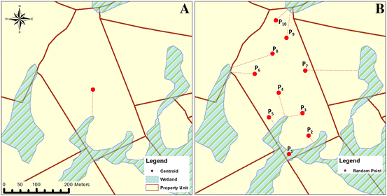

  

  Proximity to wetland methods; a centroid method; b random-points method using 10 points

• 2. Random-points method: A set of 100 points is randomly distributed over the area of a geographic unit, and the shortest Euclidean distance between every point and the closest point along the border of the nearest wetland is calculated. Thereafter, the median value of all 100-point distances is calculated (Fig. 3b).

The centroid method is simpler to calculate. For many applications, this type of definition of proximity is reasonable, especially for large distances. However, if the wetlands are located close to or even within the geographic units, which often occurs in our study, this simple method for estimating proximity has limitations (Pantazatou 2016). For example, a small wetland near the centroid will be treated as a higher exposure than several wetlands surrounding the property unit. For this distribution of wetlands, the random point method likely produces a different result (cf. Fig. 3). Another limitation of this method is that the centroid might fall outside the geographic unit, e.g., if the geometric object is composed of multiple disjoint polygons or if a polygon is horseshoe shaped (cf. Yan et al. 2006).

3.3.3 Population Density Measure

Population density can be defined using a local method in which the values for each geographic unit are calculated using only the input values for that unit. Commonly, such a measure is defined as the population divided by the area of the geographic unit. Another approach uses a geographically weighted measure in which the population densities of neighbouring units are also considered in the calculation. Finally, detailed information on the house and household level can also be used to create indexes for population density and crowding (e.g., Osei and Duker 2008). In our study, we use the two former population density measures, which are henceforth known as unweighted population density and Geographically Weighted Population Density (GWPD).

3.3.3.1 Distribution of Person-Time on Property Unit Polygons

To estimate the annual population of every property unit, the person-time of the studied population is distributed over the geographic units. Person-time is a concept used in survival analyses, and it represents the summarized time contribution of the individuals in the study population that have been exposed to or are at risk of experiencing the outcome of interest. In this study, we measure the person-time in years, which is henceforth known as person-years. In this study, we use the summarized number of years for the entire geocoded study population to produce more realistic population density measures. In other words, we include records that could be geocoded to both property units and address units (as in the variable comparisons and the survival analyses) as well as records that have only been geocoded to address units. Thus, for each year, the summarized person-years geocoded to geographic units are used to estimate the population density. The person-years are distributed based on the geographic level used.

Property Unit Level First, the person-years that are geocoded to the exact property unit are summarized for each year and property unit. Second, the person-years that are geocoded only to address units are distributed on the property units (which constitute the address units) according to the relative size of the property unit and how many person-years that have already been linked to the property unit in the first step. Thus, we make two assumptions when distributing the person-years linked to the address units only. First, property units have a population that is associated with their areas, i.e., large units have larger populations than small property units. Second, a property unit that already has a relatively large number of person-years linked to it (relative to its area) has a lower probability of being assigned person-years from the address unit level. For example, in Fig. 4a, 26 person-years in total are linked to the address unit Hög 4 for a certain year. Of these person-years, 10, 3 and 8 years are also linked to the exact property units of Hög 4:2, Hög 4:3 and Hög 4:4, respectively. The remaining 5 person-years are linked only to the address unit Hög 4 (i.e., we do not know the exact property unit for these years). Of these 5 years, 2.3 years are assigned to Hög 4:2 and 2.7 years are assigned to Hög 4:3 (Fig. 4b). No person-years are assigned to Hög 4:4 because the number of person-years linked to it is already greater than the person-years expected according to the size of the property unit. Thereafter, the population density is calculated for each property unit, and the individuals geocoded to these units are assigned the density values for the specific property units in which they reside.

Fig. 4

Distribution of person-years on property unit polygons; a initial state in which 21 person-years are geocoded to the property unit level, with 5 person-years geocoded to the address unit level; b distribution of the 5 remaining person-years (green colour) on the property units according to their relative area and previously linked person-years; c distribution of all 26 person-years (green colour) to the property units according to their relative area only. (Color figure online)

Object-Lifeline Addresses Here, all of the person-years that are linked to an address unit (including the person-years with links to both property units and address units and the person-years with links only to address units) are first summarized for each year and address unit. Thereafter, the person-years are distributed on the property units according to their relative size. For example, of the 26 years that have links to Hög 4 (Fig. 4a), 13, 6.5 and 6.5 years are linked to Hög 4:2, Hög 4:3 and Hög 4:4, respectively. The population density is calculated for each property unit, and the average density for each address unit is assigned to the individuals geocoded on this level.

Snapshot Address For this level, the same distribution method as that used in the object-lifeline addresses is applied except that the person-years are distributed only on the property units digitized from the economic map of 1914.

3.3.3.2 Unweighted Population Density

The unweighted population density measure is calculated for each year and defined as the total number of person-years in a geographic unit (distributed according to the description above) divided by the area in hectares of the geographic unit. For the object-lifeline and snapshot addresses, the population density is first calculated for the property units and then the annual average value for each address unit is calculated. For the snapshot addresses, only the property units from 1914 (digitized from the economic map) are used.

3.3.3.3 Geographically Weighted Population Density

Instead of modelling the population density for each geographic unit as isolated units, we include the neighbouring population densities and weighted them by distance. We define a geographically weighted population density (GWPD) as follows:

$$GWPD_{i} = \frac{{M_{i} }}{{A_{i} }} + \mathop \sum \limits_{j = 1}^{j = n} \frac{{M_{j} }}{{A_{j} }}W_{ij} ,\quad W_{ij} = e^{{ - 0.5 \cdot \left( {\frac{{d_{ij} }}{b}} \right)^{2} }}$$

(1)

where M _i denotes the person-years of the individuals who have lived in the geographical unit i, A _i is the area of unit i, M _j represents the person-time in the neighbouring geographical unit j, and A _j is the area of unit j. Additionally, W _ij is the spatial weight of the neighbouring population density implemented as a Gaussian distance function between geographic units j and i (cf. Fotheringham et al. 2003). In this function, b is the bandwidth that limits the search of neighbouring geographic units and d _ij is the Euclidean distance between the centroids of the geographic units i and j. In this study, a bandwidth of 1 km is used. Note that the GWPD is applied as a spatio-temporal measure, and only the geographic units that occur simultaneously in time with the geographic unit i may be counted as neighbours.

As for the unweighted population density measure, when calculating the GWPD on the object-lifeline and snapshot addresses, the GWPD is first calculated on the property unit level, and the annual average value is then calculated for each address.

A limitation of the GWPD method in this study is that the population density is somewhat underestimated for the geographic units situated near the borders of the five parishes (we have no information on the population density in the neighbouring parishes). Moreover, when calculating the GWPD, we define the distances as those between the centroids of the geographic units. The random-points method (or another method) could be used instead, but this approach was considered too computationally demanding.

3.4 Comparison of Geographic variables on Geographic Levels

We examine whether the geographic context variables differ and the degree of variation when the variables are calculated over geographic levels coarser than the property unit level.

These evaluations are performed by comparing the average annual absolute differences in proximity to wetlands or the population density between the property unit level and the corresponding value calculated for each of the coarser geographic levels. In addition, the average annual proximity to wetlands or population density is plotted. Because the values of the absolute differences do not follow a normal (Gaussian) distribution, 5% of the outliers in the absolute differences are removed to produce a more representative mean difference. The absolute differences between the random-points and centroid methods are also compared for each level, such as at the property unit level, for the two methods. This process was only applied for the wetland variables (the two population density methods were too different from each other to offer any meaningful comparisons). The absolute differences and average variable values are calculated using the linked data; thus, they are weighted by the distribution of person-time on each variable. Formally, the mean absolute differences for year y (µ _y ) are calculated as follows:

$$\upmu_{y} = \frac{{\mathop \sum \nolimits_{i = 1}^{i = n} \left( {\left| {PU_{i} - CU_{i} } \right|\left( {t_{1i} - t_{0i} } \right)} \right)}}{{\mathop \sum \nolimits_{i = 1}^{i = n} (t_{1i} - t_{0i} )}}$$

(2)

where $PU_{i}$ is the distance to the closest wetland in metres for observation i, $CU_{i}$ is the distance for the same observation calculated on a coarser geographic level, $t_{1i} - t_{0i}$ is the weight of the observation in which $t_{1i}$ represents the end time (in years) of the observation and $t_{0i}$ represents the start time in years of the observation, and $\mathop \sum \nolimits_{i = 1}^{i = n} \left( {t_{1i} - t_{0i} } \right)$ is the sum of the weights for all observations for one year.

Finally, the distribution of person-time values within certain threshold distances to the closest wetland (50, 100, 150, 250, 350, 500, 750, 1000, and 1500 m) are compared on the geographical levels. In this work, the percentage of correctly (relative to property units) classified time at risk within each threshold was determined for the object-lifeline addresses, snapshot addresses with object-lifeline wetlands, and snapshot addresses with snapshot wetlands. Therefore, by using the property unit level as reference, we determined the share of individuals who actually resided within a given distance to a wetland for each of the coarser geographic levels.

3.5 Survival Analysis

Survival analyses represent a standard approach used to study how living conditions and other factors affect the likelihood of experiencing demographic outcomes such as mortality. Survival analysis is a broad term that includes several methods that focus on questions related to the duration until an event occurs (e.g., death of an individual). One of the most commonly used models for estimating the relationship of covariates to a survival outcome is the Cox proportional hazards model. In this model, the hazard rate (h _i (t)), which is the conditional probability that an event occurs at a particular time (t), can be estimated by the following function:

$$h_{i} \left( t \right) = h_{0} \left( t \right)e^{{\beta_{1} x_{i1} + \cdots + \beta_{k} x_{ik} }}$$

(3)

where h ₀ (t) is the baseline hazard function, x _i represents the independent variables that affect the hazard, and β represents the parameters that describe the influences of the variables (Therneau and Grambsch 2000). In this model, the baseline hazard function is analogous to the intercept in an ordinary regression and corresponds to the probability of reaching an event (e.g., dying) when all of the explanatory variables are 0; moreover, this function is not parameterized or estimated in the model. The regression coefficients are estimated from the data and treated as independent of time. These values indicate the proportional change that can be expected in the hazard related to changes in the explanatory variables. The results of Cox models are generally presented by showing the relative hazards (or hazard ratios) and measuring the difference between groups with different values in the explanatory variables. Therefore, the relative hazards represent the difference in the hazard of the event (e.g., death) for the group under consideration relative to a reference group. For example, if sex were considered in a model that measures the hazard of death using female individuals as the reference category, a value of 1.2 would imply that males have a 20% higher risk of dying than females.

Using the Cox model, we analyse whether and how the proximity to wetlands and population density influence mortality within the study area. When analysing proximity to wetlands, the period was limited to 1859–1914 because we include temperature data which was only available from 1859. For the population density, we analyse the full period (1850-1914). For the proximity to wetlands variable, we estimate separate models for three high-risk groups: infants, children aged 1–5, and females aged 20–50 (WHO 2015). For the population density, we select children aged 1–15 who are sensitive to environmental factors (cf., e.g., Bengtsson 1999; Rocklov et al. 2014). Separate models are estimated for the geocoding levels as well as for the different methods applied to the geographic context variables.

3.5.1 Explanatory Variables

The following explanatory variables are used in the analyses.

Proximity to wetlands A categorical variable created using either the centroid or random-points method. This variable is based on whether an individual lives within a specified distance to a wetland. The following thresholds are used: 50, 100, 150, 250, 350, 500, 750 and 1000 m. Separate models are estimated for each threshold distance.

Population density A categorical variable created using either weighted or unweighted population density. Two variable groups are created based on two categorization methods: a) four categories with equal shares of person-time in years and b) three categories based on Jenks Natural Breaks (low, middle or high).

Geographic unit area A categorical variable indicating whether the unit is a small-scale farm (0-5 hectares), medium-scale farm (5–100 ha) or a large-scale farm (> 100 ha) (cf., Morell 2011). For the address units, the average area of the property units that constitute the address unit is used.

Socio-economic status (SES) This variable is based on the children’s/woman’s family access to land and their ability to support themselves with that land, i.e., land ownership above subsistence level (Bengtsson and Dribe (2010) includes a full description). The following four variable groups are created (Table 2): (a) freeholders and crown tenants with land above the minimum subsistence level; (b) noble tenants with time-limited leasing agreements on manorial lands above the subsistence level; (c) semi-landless individuals, including freeholders, crown tenants and noble tenants, with land below the subsistence level and crofters and cottagers with or without lands; and (d) landless individuals (e.g., workers, soldiers, and servants).

Table 2 Distribution of the time at risk in person-years on the explanatory variables for females aged 20–50, 1859–1914, and children aged 1–15, 1850–1914

Parish of Residence, Sex and Birth Year

Taxation value A ratio value indicating the productivity of the property unit (Swedish: Mantal).

Summer temperature A categorical variable indicating whether the average summer (June, July and August) temperature for a certain year is below or above the average summer temperature for the study period.

3.5.2 Cox Proportional Hazard Models

The following two Cox proportional hazard models are estimated to measure the impact of the proximity to wetlands and population density on mortality:

Wetland model Explanatory variables: proximity to wetlands (using the centroid or random-points method), parish of residence, SES, area, taxation value, summer temperature, sex and birth year. The proximity to wetland variable is interacted with summer temperature variable to better identify those warm summers in which the risk of exposure to malaria mosquitoes was highest. Separate models are estimated for the four geographical levels, the two types of distance estimations, and each of the buffer distances from 50 to 1000 m. In total, 64 models are estimated.

Population density model Explanatory variables: population density (weighted or unweighted), parish of residence, SES, area, taxation value, sex and birth year. Separate models are estimated for three geographical levels, the two types of population density methods, and the two types of population density categories (equal percentages and Jenks natural breaks). In total, 12 models are estimated.

We also use the Bayesian information criterion (BIC) to compare the fit of each estimated model across the geographic levels and quantification methods.

3.5.3 Descriptive Statistics

Table 2 shows the distribution of the individual time at risk (in percentages) among the categorical variables considered in this study and the average values of the continuous variables; the proximity to wetland and population density variables are shown separately in Tables 3 and 4, respectively. As observed in Table 2, the variable values are equal among the geographical levels, except for the area (which is affected by the geographic level). The unlinked group represents the share of individuals who could not be linked to the most detailed geographic level (i.e., the property unit) for a portion of or their entire life. The individuals who could not be linked to any level were often the poorest individuals, who often wandered between farms and other lodgings. Consequently, they are difficult to link to a household or property unit. Table 3 shows the distribution of person-years among the categorical proximity to wetland variables. Here, each pair of distance groups (e.g., < 50 m and ≥ 50 m), plus the Unlinked group, represents one categorical variable. Table 4 shows the distribution of person-years among the categorical population density variables. The variables in Tables 3 and 4 have been estimated in separate models for each quantification method and geographical level. In each of these models, the explanatory variables in Table 2 are included as controls.

Table 3 Distribution of the time at risk in person-years on the proximity to wetland variables for females aged 20–50, 1859–1914. Each pair of distance groups (e.g., < 50 m and ≥ 50 m), plus the Unlinked group, represent one categorical variable

Table 4 Distribution of the time at risk in person-years on the population density variables for children aged 1–15, 1850–1914

4 Results

4.1 Comparison of Geographic Variables

Figures 5a, b and 6a, b show the mean annual values of the variables proximity to wetland and population density on the property unit level, respectively. The figures also show the mean annual differences between the calculated value for each property unit and the corresponding value for the coarser geographic levels. The largest 5% of these differences are removed to create more representative values (because of the non-normal distribution of the differences). Overall, the figures indicate relatively larger differences between the quantification methods than between the geographic levels.

Fig. 5

Property unit level (PU) mean annual values of proximity to wetlands and mean annual difference between the PU and the other geographic levels: Object-lifeline addresses (OL_AU), snapshot addresses and object-lifeline wetlands (SN_AU OL_W), and snapshot addresses and snapshot wetlands (SN_AU SN_W); a centroid method. b Random-points method

Fig. 6

Property unit level (PU) mean annual values of population density and mean annual difference between the PU and the other geographic levels: Object-lifeline addresses (OL_AU) and snapshot addresses (SN_AU); a unweighted population density; b GWPD

Both of the wetland variables follow a similar temporal pattern (Fig. 5a, b). For the period 1850–1909 (excluding the last 4 years that account for most of the drainage activity), the average distances to wetlands on the property unit level are 458 and 447 m for the centroid and random-points methods, respectively. After approximately 1890, the mean distance to wetlands for the property unit level increases. The average absolute differences for the entire period between the property units and object-lifeline addresses are approximately 4% (20 m) and 5% (30 m), respectively, for the centroid and random-point methods. For the property units and snapshot addresses with object-lifeline wetlands, the average difference for the period is approximately 8% for both variables (40 m for the centroid method and 34 m for the random-points method). Finally, except for the period 1909–1914, the differences between snapshot addresses with snapshot wetlands and property units are large at 75% (335 m) and 66% (323 m) for the centroid and random-points method, respectively.

Moreover, the temporal patterns of the population density methods differ considerably between the two quantification methods, primarily between the average annual values on the property unit level (Fig. 6a, b). The wetland variables are similar to the population density variables because the absolute differences for the snapshot addresses begin to decrease starting from approximately 1880, and the absolute differences for the object-lifeline and snapshot addresses subsequently begin to converge. This observation is explained by the increasing similarity between the object-lifeline addresses and the snapshot addresses towards the end of the study period. The average differences between the property units and object-lifeline addresses for the entire period are approximately 14 and 23%, respectively, for the unweighted population density and the geographically weighted population density. For the property units and snapshot addresses, the average differences for the period are approximately 23 and 36% for the unweighted and the geographically weighted population density, respectively.

Moreover, Fig. 7 shows the differences between the centroid and random-points method for each geographic level. As observed in the figure, the choice of quantification method appears to affect the output values slightly more than the geographic level (except for the snapshot addresses with snapshot wetlands). For example, whereas the mean absolute differences between the property unit level and object-lifeline addresses vary between 20 and 30 m, the mean absolute difference between the random-points and centroid method on the property unit level varies between 30 and 40 m (36.5 m on average for the entire period). The unweighted and geographically weighted population density methods are based on different definitions and are not easily comparable; therefore, they were not included in this comparison.

Fig. 7

Mean annual differences between the centroid method and random-points method for each geographic level

4.2 Survival Analysis

4.2.1 Proximity to Wetlands

Figures 8 and 9 show the impact of proximity to wetlands on mortality for females aged 20–50 for the period 1859–1914.² The figure shows only the effects from the wetland category indicating residence within a certain threshold distance of wetlands during years with summer temperatures above average. The reference category for all cases is the one indicating residence outside the threshold distance. Controls are included for the parish of residence, social class, taxation value, geographic unit area, and birth year (not reported in the figures).

Fig. 8

Impact of proximity to wetlands on the mortality of females aged 20–50 in Scania, 1859–1914, centroid method. Each symbol represents the results from one separate Cox proportional hazard model, and their values represent the relative risk of dying for females residing within a given distance to wetlands. The hazard ratios and their 95% confidence intervals (bars) are plotted on a log scale. Subjects: 9576; deaths: 327; person-years at risk: 56,506. Controls: Parish of residence, social class, birth year, summer temperature, area, taxation value. The asterisks and hashes on top of the bars denote the significance values. ***p ≤ 0.001, **p ≤ 0.01, *p ≤ 0.05, ^# p ≤ 0.1. D = number of deaths. OL_AU = Object-lifeline addresses. SN_AU OL_W = Snapshot addresses and object-lifeline wetlands. SN_AU SN_W = and snapshot addresses and snapshot wetlands

Fig. 9

Impact of proximity to wetlands on mortality of females aged 20–50 in Scania 1859–1914, random-points method. Each symbol represents the results from one separate Cox proportional hazard model, and their values represent the relative risk of dying for females residing within a given distance to wetlands. The hazard ratios and their 95% confidence intervals (bars) are plotted on a log scale. Subjects: 9576; deaths: 327; person-years at risk: 56,506. Controls: Parish of residence, social class, birth year, summer temperature, area, taxation value. The asterisks and hashes on top of the bars denote the significance values. ***p ≤ 0.001, **p ≤ 0.01, *p ≤ 0.05, ^# p ≤ 0.1. D = number of deaths. OL_AU = Object-lifeline addresses. SN_AU OL_W = Snapshot addresses and object-lifeline wetlands. SN_AU SN_W = and snapshot addresses and snapshot wetlands

If using the centroid method (Fig. 8), significant and strong effects of proximity to wetlands on mortality were found for all of the geographic levels except for the snapshot addresses and snapshot wetlands. The magnitude and the statistical significance of the effect decrease as the threshold increases. At thresholds greater than 500 m, the effects are no longer observed. The effects and the statistical significance are stronger and more consistent for more detailed geographic geocoding levels. For small threshold distances, the number of deaths (D in the figure) is underestimated at the coarser geographic levels relative to the property unit level.

For the random-points method, the statistical power is reduced compared with the centroid method (Fig. 9). However, the direction of the effects for the variables is similar for the two methods (we also estimated models in which the average value of the random points for each property unit were calculated, but the effects and statistical power remained similar).

Figure 10 shows the comparisons of the BIC values for the wetland models, in which Figs. 10a and b show the BIC differences between the property unit level and each coarser geographic level for the centroid and random-points method, respectively. A positive BIC difference greater than 2 indicates that the model on the property unit level performs better than its coarser counterpart. A value lower than 2 indicates that the model using a coarser geographic level provides a better fit. For the centroid method (Fig. 10a), the BIC comparisons indicate a better fit for the models on the property unit level at threshold distances between 150 and 500 m. For the random-points method, small differences in BIC values are observed between the geographical levels, except at the threshold distances 350 and 500. Moreover, Fig. 10c shows the BIC comparison between the models using the centroid and random-points method for each geographic level. Here, the models using the centroid method performs overall better than the random-point models. This is most apparent for the property unit level at threshold distances between 150 and 500 m. Consequently, the BIC comparisons indicate that the best model fits are observed when using the centroid method at the most detailed geographical level.

Fig. 10

Differences in BIC values between the wetland models; a, b Differences between the property unit level and the coarser geographic levels for each analysed threshold distance; a centroid method; b random-points method; c difference between the centroid and random-points method for each geographical level and threshold. PU = Property units. OL_AU = Object-lifeline addresses. SN_AU OL_W = Snapshot addresses and object-lifeline wetlands. SN_AU SN_W = and snapshot addresses and snapshot wetlands

Table 5 shows the distribution of the person-year percentage within the specified threshold distances to the closest wetlands as estimated on each geographic level (note: the Unlinked group is excluded in the comparisons). The results are shown only for the centroid method. The table also shows the percentage of correctly (relative to property units) classified person-years within each threshold for the coarser geographic levels. This approach allows for further characterization of possible bias. The results in Table 5 show a strong underestimation of the person-years for the coarser geographical levels at the smaller thresholds. This effect is especially strong for the snapshot addresses with snapshot wetlands but weaker for the object-lifeline addresses. For example, of the 2735 person-years (7.06% of 38,876 person years) that are within 50 m from wetlands, 1854 person-years were correctly classified using object-lifeline addresses, 1111 person-years were correctly classified using snapshot addresses with object-lifeline wetlands, and only 190 person-years were correctly classified using snapshot addresses with snapshot wetlands. At distances of 350 m and larger, at least 95% of the object-lifeline addresses are located within the same distance category as the property units. Overall, this result means that at small distances, the estimated number of persons at-risk is much lower compared with that of the property units. For these smaller buffer radiuses, the results suggest that the coarser levels are inaccurate. This result is expected because the object-lifeline address units and snapshot addressees with object-lifeline wetlands deviate by approximately 20 and 50 m, respectively, from the distances calculated on the property units.

Table 5 Differences between geocoding levels in determining females aged 20–50 being exposed to wetlands based on centroid method (Unlinked group excluded). Period 1850–1914

4.2.2 Population Density

Figures 11 and 12 show the impact of population density on child mortality for the period 1850–1914. In these figures, each box represents one Cox proportional hazard model. Two types of variable categorizations have been used, with one based on equal shares of the percentage of person-years and one on the Jenks Natural Breaks. Using the GWPD method (Fig. 11), significant effects on child mortality are found for the property units and the snapshot addresses. Moreover, the pattern of the effects are similar across the all of the geographical levels. Note also that the significance of the effects are slightly stronger for the snapshot addresses compared with the property units when using the Jenks Natural Breaks. Lastly, using the unweighted population density, no significant effects are found (Fig. 12).

Fig. 11

Impact of the population density on child mortality in Scania from 1850 to 1914, GWPD method. Each box represents the results from one separate Cox proportional hazard model. The values represent the relative risk of dying for children residing in an area with a given category of the weighted population density. Note that the hazard ratios and their 95% confidence intervals (the bars) are plotted on a log scale. Subjects: 17,647; deaths: 1118; person-years at risk: 109,353. Controls: Parish of residence, social class, birth year, property unit area, taxation value. The asterisks and hashes on top of the bars denote the significance values. ***p ≤ 0.001, **p ≤ 0.01, *p ≤ 0.05, ^# p ≤ 0.1. D = number of deaths. PU = Property units. OL_AU = Object-lifeline addresses. SN_AU = Snapshot addresses

Fig. 12

Impact of population density on child mortality in Scania 1850–1914, unweighted population density method. Each box represents the results from one separate Cox proportional hazard model. The values represent the relative risk of dying for children residing in an area with a given category of the weighted population density. Note that the hazard ratios and their 95% confidence intervals (the bars) are plotted on a log scale. Subjects: 17,647; deaths: 1118; person-years at risk: 109,353. Controls: Parish of residence, social class, birth year, property unit area, taxation value. The asterisks and hashes on top of the bars denote the significance values. ***p ≤ 0.001, **p ≤ 0.01, *p ≤ 0.05, ^# p ≤ 0.1. D = number of deaths. PU = Property units. OL_AU = Object-lifeline addresses. SN_AU = Snapshot addresses

Figure 13 shows the comparisons of the BIC values for the population density models. Figure 13a and b show the BIC differences between the property unit level and each coarser geographic level for the GWPD and unweighted population density, respectively. As indicated also in Fig. 11, the models on snapshot addresses provide a better fit compared to the models on the property unit level. Moreover, models using the GWPD method performs consistently better than the models using the unweighted population density (Fig. 13c). Thus, the results from Figs. 11, 12 and 13 indicate that the type of method used in this paper appears to influence the outcome of the survival analysis to a greater extent than the geographical level.

Fig. 13

Differences in BIC values between the population density models; a, b differences between the property unit level and the coarser geographic levels for each categorization method; a GWPD; b unweighted population density; c difference between the GWPD and unweighted population density for each geographical level and categorization method

5 Discussion and Conclusions

The main aim of this study was to analyse how evaluations of the impact of geographic context variables on demographic longitudinal analyses are affected by the geographic levels of the geocoding and the method used to quantify the geographic context variables. We summarise three major findings. First, even relatively small differences between the property units and the coarser geographic levels influenced both the magnitude of the effect and the statistical power in the survival analyses. For example, the period-average difference between the property units and object-lifeline addresses was only 4% (20 m) when using the centroid method; however, such differences still influenced the survival analyses. Nonetheless, when analysing the mortality effects of the geographic variables proximity to wetlands and population density, relationships were observed in the survival analyses at those coarser geographical levels. For example, for the proximity to wetlands variable, statistically significant effects on mortality were not only found at the property unit level, but also at the object-lifeline address level, and snapshot addresses with object-lifeline wetland level. However, the coarser levels underestimated the number of persons at risk in analyses performed at distances of less than approximately 350 m. Conclusively, the coarser geographic levels might not be appropriate for such fine-scale analyses. Second, our study shows the importance of accounting for any substantial changes in time, both in the geographic data used to geocode the population and in any external data used to calculate the context variables, such as the drainage of wetlands. Third, the choice between common methods used to quantify the geographic context variables substantially influenced the results of the survival analyses, which was occasionally greater than the influence of the geographic level.

In fine-scale analyses, the coarser geographic levels used in this study might not be suitable. This statement primarily applies to the proximity to wetlands variable. For example, the distances calculated for the object-lifeline addresses and snapshot addresses with object-lifeline wetlands levels differed by approximately 20 and 50 m, respectively, from those calculated on the property unit level. Although such differences might appear small, they resulted in substantial underestimations of the number of individuals at-risk in analyses performed at small distances of up to at least 350 m. Hence, serious bias can be introduced in the analyses if these coarser geographical levels are used to analyse the effects and identify the patterns at small distances. In addition, the statistical significance of the effects was stronger and more consistent, and the models performed better (according to the BIC comparison), for more detailed geographic geocoding levels. Therefore, the exact property unit level is better suited for such fine-scale analyses to estimate reliable models and identify relationships between variables on the micro-level.

In general, the method used to quantify the geographic factors had a larger influence on the results of the survival analyses than the geographical level of the geocoding. This result is observed in the different patterns of the two population density methods (Fig. 6), in the larger absolute differences between the random-points and centroid methods compared with the differences between geographic levels (Figs. 5, 7), in the different statistical powers in the results from the survival analysis (Figs. 8, 9, 11, 12), and in the BIC comparisons (Figs. 10, 13). For example, whether the population density is geographically weighted or not can produce notably different results and model fits. Thus, appropriate definitions of the geographic context must be used. Otherwise, important relationships might remain unidentified, and the high spatial resolution in the geocoding cannot be properly utilized. When analysing the effect of exposure to diseases, such as in our case, the geographically weighted population density is generally a more appropriate method than the unweighted population density method (which treats each geographic unit as an isolated area) (e.g., Cromley and McLafferty 2011). To the best of our knowledge, this study is also one of the first to use such a method when analysing spatio-temporal micro-level data. For the proximity to wetlands variable sufficient information is not available to determine the method that is the most appropriate for the analyses performed in this study (although the BIC comparisons indicated that the centroid method may be more appropriate than the random-points method). If we hypothesize that proximity to wetlands in the study area increases the exposure to malaria mosquitoes, such exposure would be highest between dusk and dawn (WHO 2015). In this case, an appropriate quantification method will accurately estimate the location of the individuals during this time of the day, such as inside and around residential buildings. In this case, the centroid method might better correspond to the place of residence within the property unit, whereas the random-point method might better represent the location of the individuals during the daytime. However, we have not tested this assumption. In addition, studies using modern data have found relatively large average differences between the centroid of a rural property unit and the residential building within it (RMSE = 211 m) (Cayo and Talbot 2003). Consequently, more context-specific considerations are required to determine the appropriateness of the quantification methods used in this study.

Moreover, geographic variables estimated using external geographic data are obviously heavily influenced by the spatio-temporal quality of such data. In our study, calculating the distances to wetlands using only snapshot information from the end of the study period substantially influenced the results of the survival analysis primarily because the snapshot data did not contain information on the substantial drainage activities that had been performed in the area (however, this effect would likely be smaller if we used older snapshot information from military topographic maps from 1820 because of the abrupt decrease in the number of wetlands in 1909). Thus, large changes through time in both the geographic data used to geocode the population and in any external geographic data used to calculate the geographic context variables must be considered.

In conclusion, the findings show that the geographical level used for geocoding is important for demographic analyses. Reasonably, analyses at more detailed levels require a higher quality of data. In our case, if we are interested in dynamic variables operating at distances of under hundreds of metres, we would have to perform analyses on the property unit level to estimate more reliable models. The suitable geographic level for geocoding is nevertheless context dependent. Selected geographic factors operate on a local scale, whereas others operate on coarser scales. Certain factors change frequently with time, whereas others are static. In general, one must consider the distances of interest for the analysis and the phenomena under study. For geographic context variables, we must also consider the quantification methods that are the most logical for the type of analyses. For example, we might need to use different methods for the population density parameter depending on whether exposure to virulent airborne diseases or poor sanitation is analysed and whether the geographic context is static or dynamic. Therefore, to offer a general recommendation on the geographic level for the geocoding, the future use of the demographic database to be geocoded must be known. If possible, the geographic level that supports the most demanding use of the database should be applied. However, a lack of historical sources and shortages in economic resources might present limitations for geocoding; thus, the introduction of such limitations into demographic analyses should be identified.

References

Bengtsson, T. (1999). The vulnerable child. Economic insecurity and child mortality in pre-industrial Sweden: A case study of Västanfors, 1757–1850. European Journal of Population/Revue Européenne de Démographie, 15(2), 117–151.
Bengtsson, T., & Dribe, M. (1997). Economy and demography in Western Scania, Sweden, 1650–1900. Eurasian project on population and family history working paper series, No. 10. Kyoto: International Research Center for Japanese Studies.
Bengtsson, T., & Dribe, M. (2010). Quantifying the family frailty effect in infant and child mortality by using median hazard ratio (MHR). Historical Methods: A Journal of Quantitative and Interdisciplinary History, 43(1), 15–27.
Bengtsson, T., & Dribe, M. (2011). The late emergence of socioeconomic mortality differentials: A micro-level study of adult mortality in southern Sweden 1815–1968. Explorations in Economic History, 48(3), 389–400.
Bengtsson T., Dribe M., Quaranta L., & Svensson P. (2014). The Scanian Economic Demographic Database, Version 4.0 (Machine-readable database), C.f.E.D. Lund University, Lund.
Cayo, M. R., & Talbot, T. O. (2003). Positional error in automated geocoding of residential addresses. International Journal of Health Geographics, 2(1), 1.
Claësson, O. (2009). Geographical differences in infant and child mortality during the initial mortality decline: Evidence from southern Sweden, 1749–1830. Lund: Department of Economic History, Centre for Economic Demography, Lund University.
Cromley, E. K., & McLafferty, S. L. (2011). GIS and public health. Guilford Press.
DeBats, D. A. (2011). Political consequences of spatial organization. Social Science History, 35(04), 505–541.
Delmelle, E., Dony, C., Casas, I., Jia, M., & Tang, W. (2014). Visualizing the impact of space–time uncertainties on dengue fever patterns. International Journal of Geographical Information Science, 28(5), 1107–1127.
Ekamper, P. (2010). Using cadastral maps in historical demographic research: Some examples from the Netherlands. History of the Family, 15(1), 1–12.
Feitosa, F. F., Camara, G., Monteiro, A. M. V., Koschitzki, T., & Silva, M. P. (2007). Global and local spatial indices of urban segregation. International Journal of Geographical Information Science, 21(3), 299–323.
Flowerdew, R., Manley, D. J., & Sabel, C. E. (2008). Neighbourhood effects on health: Does it matter where you draw the boundaries? Social Science and Medicine, 66, 1241–1255.
Fotheringham, A. S., Brunsdon, C., & Charlton, M. (2003). Geographically weighted regression: The analysis of spatially varying relationships. New York: Wiley.
Gregory, N. (2008). Different places, different stories: Infant mortality decline in England and Wales, 1851–1911. Annals of the Association of American Geographers, 98(4), 773–779.
Griffith, D. A., Millones, M., Vincent, M., Johnson, D. L., & Hunt, A. (2007). Impacts of positional error on spatial regression analysis: A case study of address locations in Syracuse, New York. Transactions in GIS, 11(5), 655–679.
Gutmann, M. P., Deane, G. D., Lauster, N., & Peri, A. (2005). Two population-environment regimes in the great plains of the United States, 1930–1990. Population and Environment, 27(2), 191–225.
Hedefalk, F., Harrie, L., & Svensson, P. (2015). Methods to create a longitudinal integrated demographic and geographic database on the micro-level a case study of five Swedish rural parishes, 1813–1914. Historical Methods: A Journal of Quantitative and Interdisciplinary History, 48(3), 153–173.
Hedefalk, F., Quaranta, L., & Bengtsson, T. (2017a). Unequal lands: Soil type, nutrition and child mortality in southern Sweden, 1850–1914. Demographic Research, 36, 1039–1080.
Hedefalk, F., Svensson, P., & Harrie, L. (2017b). Spatiotemporal historical datasets at micro-level for geocoded individuals in five Swedish parishes, 1813–1914. Scientific Data, 4, 170046.
Jacquez, G. M. (2012). A research agenda: Does geocoding positional error matter in health GIS studies? Spatial and spatio-temporal epidemiology, 3(1), 7–16.
Kang, S. Y., McGree, J., & Mengersen, K. (2014). The choice of spatial scales and spatial smoothness priors for various spatial patterns. Spatial and Spatio-temporal Epidemiology., 10, 11–26.
Kasakoff, A. B., Lawson, A. B., Dasgupta, P., Feetham, S., & DuBois, M. J. (2013). Spatial inequality in wealth: A Bayesian analysis of the Northeastern US in 1860—Does space matter. Spatial Demography, 1(1), 56–95.
Kwan, M.-P. (2012). The uncertain geographic context problem. Annals of the Association of American Geographers, 102, 958–968.
Lazuka, V., Quaranta, L., & Bengtsson, T. (2016). Fighting infectious disease: Evidence from Sweden 1870–1940. Population and Development Review, 42(1), 27–52.
Lindgren, E., & Jaenson, T. G. (2006). Fästing-och myggöverförda infektionssjukdomar i ett kommande, varmare klimat i Sverige. Ent. Tidskr, 127, 21–30.
Logan, J. R. (2012). Making a place for space: Spatial thinking in social science. Annual Review of Sociology, 38(1), 507–524.
Mazumdar, S., Rushton, G., Smith, B. J., Zimmerman, D. L., & Donham, K. J. (2008). Geocoding accuracy and the recovery of relationships between environmental exposures and health. International Journal of Health Geographics, 7(1), 1.
Morell, M. (2011). Agriculture in industrial society: 1870-1945. In J. Myrdal & M. Morell (Eds.), The agrarian history of Sweden: from 4000 BC to AD 2000 (pp. 165–213). Lund: Nordic Academic Press.
Openshaw, S., & Openshaw, S. (1984). The modifiable areal unit problem. Geo Abstracts University of East Anglia.
Osei, F. B., & Duker, A. A. (2008). Spatial and demographic patterns of cholera in Ashanti region-Ghana. International Journal of Health Geographics, 7(1), 1.
Pantazatou K.D. (2016). Issues of Geographic Context Variable Calculation Methods applied at different Geographic Levels in Spatial Historical Demographic Research—A case study over four parishes in Southern Sweden (Master’s thesis). Lund University, Lund, Sweden.
Parker, M., Matthews, S. A., Yan, G., Zhou, G., Lee, M.-C., Sirichaisinthop, J., et al. (2015). Microgeography and molecular epidemiology of malaria at the Thailand-Myanmar border in the malaria pre-elimination phase. Malaria Journal, 14, 198.
Pezeshki, Z., Tafazzoli-Shadpour, M., Mansourian, A., Eshrati, B., Omidi, E., & Nejadqoli, I. (2012). Model of cholera dissemination using geographic information systems and fuzzy clustering means: Case study, chabahar, Iran. Public Health, 126(10), 881–887.
Reardon, S. F., & O’Sullivan, D. (2004). Measures of spatial segregation. Sociological Methodology, 34(1), 121–162.
Rocklov, J., Edvinsson, S., Arnqvist, P., de Luna, S. S., & Schumann, B. (2014). Association of seasonal climate variability and age-specific mortality in northern Sweden before the onset of industrialization. International Journal of Environmental Research and Public Health, 11(7), 6940–6954.
Root, G. (1997). Population density and spatial differentials in child mortality in Zimbabwe. Social Science and Medicine, 44(3), 413–421.
Ruggles, S., Roberts, E., Sarkar, S., & Sobek, M. (2011). The North Atlantic population project: Progress and prospects. Historical Methods: A Journal of Quantitative and Interdisciplinary History, 44(1), 1–6.
Staedke, S. G., Nottingham, E. W., Cox, J., Kamya, M. R., Rosenthal, P. J., & Dorsey, G. (2003). Short report: Proximity to mosquito breeding sites as a risk factor for clinical malaria episodes in an urban cohort of Ugandan children. The American Journal of Tropical Medicine and Hygiene, 69(3), 244–246.
Therneau, T. M., & Grambsch, P. M. (2000). Modeling survival data: Extending the Cox model. New York: Springer.
Vieira, V. M., Howard, G. J., Gallagher, L. G., & Fletcher, T. (2010). Geocoding rural addresses in a community contaminated by PFOA: A comparison of methods. Environmental Health, 9(1), 1.
Villarreal, C., Bettenhausen, B., Hanss, E., & Hersh, J. (2014). Historical health conditions in major US Cities: The HUE data set. Historical Methods: A Journal of Quantitative and Interdisciplinary History, 47(2), 67–80.
Voss, P. R. (2007). Demography as a spatial social science. Population Research and Policy Review, 26(5–6), 457–476.
Woods, R. (2003). Urban-rural mortality differentials: An unresolved debate. Population and development review, 29, 29–46.
Worboys, M. F., & Duckham, M. (2004). GIS: A computing perspective. Boca Raton, FL: CRC Press.
World Health Organization (WHO). (2015). World Malaria Report 2015. http://apps.who.int/iris/bitstream/10665/200018/1/9789241565158_eng.pdf?ua=1.
Xu, H., Logan, J. R., & Short, S. E. (2014). Integrating space with place in health research: A multilevel spatial investigation using child mortality in 1880 Newark, New Jersey. Demography, 51(3), 811–834.
Yan, H., Chu, Y., Li, Z., & Guo, R. (2006). A quantitative description model for direction relations based on direction groups. Geoinformatica, 10(2), 177–196.
Zandbergen, P. A. (2007). Influence of geocoding quality on environmental exposure assessment of children living near high traffic roads. BMC Public Health, 7(1), 1–13.
Zandbergen, P. A. (2008). A comparison of address point, parcel and street geocoding techniques. Computers, Environment and Urban Systems, 32(3), 214–232.
Zandbergen, P. A. (2009). Geocoding quality and implications for spatial analysis. Geography Compass, 3(2), 647–680.
Zhou, G., Munga, S., Minakawa, N., Githeko, A. K., & Yan, G. (2007). Spatial relationship between adult malaria vector abundance and environmental factors in western Kenya highlands. The American Journal of Tropical Medicine and Hygiene, 77(1), 29–35.
Acknowledgements
This study was a collaboration between the Centre for Economic Demography (CED) and the Department of Physical Geography and Ecosystem Science (INES) as part of the eSSENCE project financed by the Swedish Research Council. The authors also thank the anonymous reviewers for constructive feedback that improved the quality of this paper. Author x.x is also grateful for funding provided by the Jan Wallander and Tom Hedelius Foundation and by the project “Growth and inequality before the industrial revolution”, funded by the Swedish Research Council.
Author information
Authors and Affiliations
Corresponding author
Ethics declarations
Conflict of interest
On behalf of all authors, the corresponding author states that there is no conflict of interest.
Rights and permissions
Open Access This article is distributed under the terms of the Creative Commons Attribution 4.0 International License (http://creativecommons.org/licenses/by/4.0/), which permits unrestricted use, distribution, and reproduction in any medium, provided you give appropriate credit to the original author(s) and the source, provide a link to the Creative Commons license, and indicate if changes were made.
About this article
Cite this article
Hedefalk, F., Pantazatou, K., Quaranta, L. et al. Importance of the Geocoding Level for Historical Demographic Analyses: A Case Study of Rural Parishes in Sweden, 1850–1914. Spat Demogr 6, 35–69 (2018). https://doi.org/10.1007/s40980-017-0039-7
Published:
Issue Date:
DOI: https://doi.org/10.1007/s40980-017-0039-7