Multiplication of distributions and singular waves in several physical models

Abstract

We study of a Riemann problem for a one-dimensional $2\hspace{1.111pt}{\times }\hspace{1.111pt}2$ system of conservation laws, which includes some particular cases of known physical systems, such as the pressureless gas dynamics system, Euler equations for isentropic flow, the Brio system, and the shallow water system. The main results of this study reveal the emergence of shock waves and delta shock waves as explicit solutions. We use the concept of $\alpha$-solution defined in the setting of a product of distributions not defined by approximation. Notably, this study does not assume any classical results about conservation laws, presenting a simpler and more general framework for constructing singular solutions to other equations or systems. Additionally, this paper includes several comments on the four physical systems mentioned, along with formulas for multiplying distributions and evaluating the compositions of a function with a distribution.

1 Introduction

Physical problems typically involve highly complex mathematical frameworks and it is necessary to use simplified models in order to deal with these phenomena. Some of these models employ conservation laws systems such as the following:

$$\begin{aligned} \begin{aligned} u_{t}+\biggl [ \frac{u^{2}}{2}+\phi (v)\biggr ]_{x}&=0,\\ v_{t}+[(u-k)\hspace{1.111pt}\psi (v)]_{x}&=0, \end{aligned} \end{aligned}$$

(1)

where $u=u(x,t)\in {\mathbb {R}}$, $v=v(x,t)\in {\mathbb {R}}$ are unknown state variables, $x,t\in {\mathbb {R}}$ are, respectively, the space and time variables, $\phi ,\psi :{{\mathbb {R}}}\rightarrow {{\mathbb {R}}}$ are functions and k is a real constant. Notably, this system includes the pressureless gas dynamics system, the Euler equations for the isentropic flow, the shallow water system, and the Brio system as particular cases.

In this paper we study system (1) subject to the initial conditions

$$\begin{aligned} u(x,0) =u_{1}+(u_{2}-u_{1})H(x),\quad v(x,0) =v_{1}+(v_{2}-v_{1})H(x), \end{aligned}$$

(2)

where H stands for the Heaviside function and $u_{1},u_{2},v_{1},v_{2}\in {\mathbb {R}}$ (Riemann problem).

Motivated by the results obtained in [4, 5, 11, 21], among others, we begin to seek for solutions in the space ${{\mathscr {W}}}$ of pairs of distributions (u, v) defined by

$$\begin{aligned} u(x,t)&=f(t)+g(t)H(x-\gamma (t))+h(t)\hspace{1.111pt}\delta (x-\gamma (t)),\\ v(x,t)&=a(t)+b(t)H(x-\gamma (t)), \end{aligned}$$

where $f,g,h,a,b,\gamma :\mathbb {R\rightarrow R}$, with $\gamma (0)=0$, are $C^{1}$-functions and $\delta$ stands for the Dirac measure supported at the origin. Here, we assume $\phi$ and $\psi$ without any restrictions.

Furthermore, assuming that $\phi$ and $\psi$ have an extension into the complex plane as entire functions, we are also able to study problem (1)–(2) in the space ${{\mathscr {W}}}_{1}$ of pairs of distributions (u, v) defined by

$$\begin{aligned} u(x,t)&=f(t)+g(t)H(x-\gamma (t)),\\ v(x,t)&=a(t)+b(t)H(x-\gamma (t))+c(t)\hspace{1.111pt}\delta (x-\gamma (t)), \end{aligned}$$

where $f,g,a,b,c,\gamma :\mathbb {R\rightarrow R}$, with $\gamma (0)=0$, are $C^{1}$-functions.

Following [20, 21, 23, 24], we use the so-called $\alpha$-solution theory, developed by Sarrico, and, consequently, we adopt the $\alpha$-solution concept, which is defined within a product of distributions (the $\alpha$-product). This product associates to certain pairs of distributions (T, S) another distribution represented by $T_{\dot{\alpha }}S$, which depends on a function $\alpha \in {\mathscr {D}}$ such that $\int _{-\infty }^{+\infty } \alpha (x)\hspace{0.55542pt}\textrm{d}x =1$ (here it is sufficient to consider the dimension $N=1$). The function $\alpha$ encodes the inherent indeterminacy present in certain products of distributions. Furthermore, this product enables us to define certain compositions of functions with distributions.

The $\alpha$-solution concept generalises the classical solution concept and can be seen as a new type of weak solution in the nonlinear setting. A detailed explanation of the $\alpha$-solution concept for a particular case of system (1) can be found in [22, p. 339].

Our main results are the emergence of shock waves and $\delta$-shock waves in explicit form which can be seen in Theorems 4.1 and 5.1. Notably, such $\alpha$-solutions do not depend on $\alpha$, and using the $\alpha$-product of distributions they can be directly substituted into the systems!

The presence of $\delta$-shock solutions in certain Riemann problems associated with conservation laws systems is a well-known phenomenon (see [2]). Korchinski [7] was one of the pioneers, back in 1977, to introduce these solutions in the system $u_{t}+(u^{2})_{x}=0$, $v_{t}+(uv)_x=0$. However, it was only in 2010 that experimental evidence of these waves was obtained [8].

The $\alpha$-solution method (due to Sarrico) represents a significant advance in the study of singular solutions of nonlinear equations or systems. One of the key advantages of this method is the fact that, despite the possible $\alpha$-dependence of these solutions, for many initial value problems, the $\alpha$-solutions remain independent of $\alpha$. This feature has led to an increasing adoption of the method by various authors, as evidenced by recent publications such as [11,12,13,14, 26,27,28,29].

Another advantage of the $\alpha$-solution method regards the framework of Rankine–Hugoniot shock conditions and their generalizations; as far as we know, these conditions are not necessary, and the final result is the same (see, for example, [12, 17, 18]).

Finally, we draw attention to the paper [14], which provides the first numerical simulations of a Riemann problem involving $\delta '$-shock waves using the Nessyahu–Tadmor scheme [10]. The results of this study are successfully compared with exact solutions obtained using the $\alpha$-solution method.

Regarding to the physical models mentioned before, the Brio system

(3)

is a simplified model for the study of plasmas and corresponds to the coupling of the fluid dynamic equations with Maxwell’s equations of electrodynamics. Subjecting u, v to the initial conditions (2), it was already shown by Sarrico [21], in 2015, the existence of a unique explicit solution in ${{\mathscr {W}}}$. Naturally, we reobtain it in the present paper, taking $\phi (v)={v^{2}}/{2}$, $k=1$ and $\psi (v)=v$, in (1). This solution and also the one obtained in ${{\mathscr {W}}}_1$ coincide with the ones obtained, in 2012, by Kalisch and Mitrovic in [4, Theorem 3.1] using the so-called weak asymptotic method.

The shallow-water system

(4)

is a simplified model for the study of surface waves in an inviscid fluid that propagates in a channel of uniform width and little depth. Here, $u=u(x,t)$ stands for the horizontal fluid speed and $v=v(x,t)$ denotes the height of the water surface above a horizontal bottom which we considered flat. It is assumed that u is independent of the depth and r is a gravitational constant. Taking $\phi (v)=rv$, $k=0$, $\psi (v)=v$, in (1), we will see that, with the initial conditions (2), our solution in ${{\mathscr {W}}}$ coincides with the one obtained by Kalisch, Mitrovic and Teyekpiti [5, Theorem 2.2], in 2017, using the assymptotic method. The existence and uniqueness result to problem (4) in ${{\mathscr {W}}}$ was already obtained in 2018, by Sarrico and Paiva [23], and can be seen as a particular case of our Theorem 4.1. It is worth noting that the inclusion of Dirac-delta distributions into the shallow-water theory was done by Edwards et al. in [2] and physical interpretation can be found in [3].

If we consider $k=0$ and $\psi (v)=v$ in (1), we get

(5)

which is a particular case of the Euler equations for the isentropic flow, in one dimension. In this model, $u=u(x,t)$ stands for the velocity of the fluid, $v=v(x,t)$ denotes its density, and $\phi$ is a function related with the pressure P (function of the density, determined from the constitutive thermodynamic relations of the fluid under consideration), namely $P'(v)=v\phi '(v)$. The Euler’s equations in fluid dynamics describe the flow of an inviscid and incompressible fluid. Considering the initial conditions (2) we prove the existence of a unique solution in ${{\mathscr {W}}}$ which coincides with the one obtained by Paiva in 2020, [11]. We also obtain a unique solution in ${{\mathscr {W}}}_1$ that coincides with the one obtained by Sarrico and Paiva in 2017, [22].

Taking $\phi =0$ in (5) we obtain the pressureless gas dynamics system

(6)

Subjecting u, v to the same initial conditions, our solution allows us to see the development of a travelling wave that coincides with the one obtained by Sarrico in 2014, [20] (taking $\phi (u)={u^{2}}/{2}$ and $\psi (u)=u$) and also with the solution obtained by Danilov, Mitrovic and Bojkovic in [1] and [9] by two different methods.

This paper is organized as follows. In Sect. 2, we list some results related to the $\alpha$-product, which we use in the rest of the paper. In Sect. 3, we introduce the concept of $\alpha$-solution for system (1). Sections 4 and 5 state and prove our main results. In Sect. 6, we give some comments on what we said regarding the four physical systems mentioned.

2 Some auxiliary results concerning the $\alpha$-products

In this section, we provide a brief overview of $\alpha$-products, denoted by $_{\dot{\alpha }}$. For more details and properties related to these products, we refer the interested reader to [16, 18, 20,21,22] or [15].

We begin with some notation. Let ${\mathscr {D}}$ be the space of real- or complex-valued functions that are infinitely differentiable and have compact support on ${{\mathbb {R}}}$. The space of Schwartz distributions, denoted by ${\mathscr {D}}^{\prime }$, is the topological dual of ${\mathscr {D}}$. Additionally, we consider ${\mathscr {D}}^{\prime p}$ as the space of distributions of order $\leqslant p$, in the sense of Schwartz, where $p\in \{0,1,2,\dots ,\infty \}$. ${\mathscr {D}}^{\prime \infty }$ means ${\mathscr {D}}^{\prime }$. Moreover, ${\mathscr {D}}_{\mu }^{\prime }$ denotes the space of distributions whose support has zero Lebesgue measure, and ${\mathscr {D}}_{\textrm{c}}^{\prime }\subset {\mathscr {D}}_{\mu }^{\prime }$ is the space of distributions whose support is at most countable.

From now on, we consider $\alpha \in {{\mathscr {D}}}$ such that $\int _{-\infty }^{+\infty } \alpha (x)\hspace{0.55542pt}\textrm{d}x =1$, and for the sake of simplicity we introduce the following notations:

The $\alpha$-products, in general, are neither associative nor commutative (we recall that the so-called classical products of distributions are not associative and commutativity is a convention, see [25, pp. 117, 118, 121]), but they are bilinear, they satisfy the usual differential rules. In particular, the Leibniz formula must be written as follows (D represents the usual derivative in a distributional sense):

$$\begin{aligned} D(T_{\dot{\alpha }}S)=(DT)_{\dot{\alpha }} S+ T_{\dot{\alpha }}(DS), \end{aligned}$$

for $T,S \in {\mathscr {D}}^{\prime }$. Additionally, translations act in the usual way, which means that

$$\begin{aligned} \tau _c(T_{\dot{\alpha }}S)=(\tau _c T)_{\dot{\alpha }}(\tau _cS), \end{aligned}$$

(7)

where $c\in {{\mathbb {R}}}$ and $\tau _c$ stands for the usual translation operator in the distributional sense.

We present three $\alpha$-products formulae that we need to study our system (1).

• (I) If $T\in {\mathscr {D}}^{\prime -1}$ and $S=\beta +f\in C^{p}\hspace{0.55542pt}{\oplus }\hspace{1.111pt}{\mathscr {D}}_{\mu }^{\prime }$, with $p\in \{0,1,2,\dots ,\infty \}$, the $\alpha$-product $T_{\dot{\alpha }}S$ is given by

  $$\begin{aligned} T_{\dot{\alpha }}S=T\beta +(T\hspace{1.111pt}{*}\hspace{1.111pt}\alpha )f. \end{aligned}$$

  (8)

  In this formula $T\beta$ represents the usual product of a ${\mathscr {D}}^{\prime p}$ distribution with a $C^p$-function and $(T\hspace{1.111pt}{*}\hspace{1.111pt}\alpha )f$ stands for the usual product of a $C^\infty$-function with a distribution.

  Using (8), we can now compute

  $$\begin{aligned} \delta _{\dot{\alpha }}\delta =\delta _{\dot{\alpha }}(0+\delta )=\delta 0+(\delta \hspace{1.111pt}{*}\hspace{1.111pt}\alpha )\hspace{1.111pt}\delta =\alpha \delta =\alpha (0)\hspace{1.111pt}\delta , \end{aligned}$$

  (9)

  and also

  

  (10)

• (II) If $T\in {\mathscr {D}}^{\prime -1}$ and $S=w+f\in L_\textrm{loc}^{1}\hspace{0.55542pt}{\oplus }\hspace{1.111pt}{\mathscr {D}}_{\mu }^{\prime }$, where ${\mathscr {D}}^{\prime -1}$ stands for the space of distributions $J\in {\mathscr {D}}^{\prime }$ such that DJ $\in {\mathscr {D}}^{\prime 0}$, then the $\alpha$-product $T_{\dot{\alpha }}S$ is defined by

  $$\begin{aligned} T_{\dot{\alpha }}S=T_{\dot{\alpha }}(w+f) =Tw+(T\hspace{1.111pt}{*}\hspace{1.111pt}\alpha )f, \end{aligned}$$

  (11)

  where Tw is the usual pointwise product of $T\in {\mathscr {D}}^{\prime -1}$ with $w\in L_\textrm{loc}^{1}$ (remember that, locally, T can be seen as a bounded variation function).

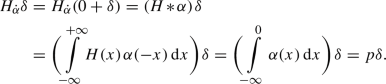
  We can apply (11) to compute $H_{\dot{\alpha }}H$. Since $H\in {\mathscr {D}}^{\prime -1}$ and $H=H+0\in L_\textrm{loc}^{1}\hspace{0.55542pt}{\oplus }\hspace{1.111pt}{\mathscr {D}}_{\mu }^{\prime }$, from (11), we have

  $$\begin{aligned} H_{\dot{\alpha }}H=HH+(H\hspace{1.111pt}{*}\hspace{1.111pt}\alpha )\hspace{1.111pt}0=H. \end{aligned}$$

  (12)

  More generally, if $T\in {\mathscr {D}}^{\prime -1}$ and $S\in L_\textrm{loc}^{1}$, then $T_{\dot{\alpha }}S=TS$, that is, in this case, the $\alpha$-product coincides with the usual pointwise product.

• (III) Finally, if $T\in {\mathscr {D}}^{\prime 0}\cap {\mathscr {D}}_{\mu }^{\prime }$, $S,DS\in L_\textrm{loc}^{1}\hspace{1.111pt}{\oplus }\hspace{1.111pt}{\mathscr {D}}_\textrm{c}^{\prime }$, and $Y\in {\mathscr {D}}^{\prime -1}$ is such that $DY=T$, then the $\alpha$-product $T_{\dot{\alpha }}S$ is given by

  $$\begin{aligned} T_{\dot{\alpha }}S=D(Y_{\dot{\alpha }}S)-Y_{\dot{\alpha }}(DS). \end{aligned}$$

  (13)

  The $\alpha$-products $Y_{\dot{\alpha }}S$ and $Y_{\dot{\alpha }}(DS)$ may be computed by (8) or (11).

  The value of $\alpha$-product $T_{\dot{\alpha }}S$, given by (13), is independent of the choice of $Y\in {\mathscr {D}}^{\prime -1}$ such that $DY=T$ (see [19, p. 1004]). For instance, by (10) and (13), we have for any $\alpha$,

  $$\begin{aligned} \begin{aligned} \delta _{\dot{\alpha }}H=(DH)_{\dot{\alpha }}H&=D(H_{\dot{\alpha }}H)-H_{\dot{\alpha }}(DH)\\ {}&=DH-H_{\dot{\alpha }}\delta =\delta -p\delta =q\delta . \end{aligned} \end{aligned}$$

  (14)

The $\alpha$-products (I), (II), and (III) are consistent with the classical Schwartz products of ${\mathscr {D}}^{\prime p}$-distributions with $C^p$-function, if the latter are placed at the right-hand side. Furthermore, the three products are mutually compatible, meaning that whenever two of them can be calculated, the results are the same.

In our study, we also require the composition of an entire function with certains distributions. The procedure is summarized as follows (see [22] for a detailed description):

• Let $a,b,{\tilde{p}},{\tilde{q}}\in {\mathbb {C}}$ and let $P_{n}$ be the sequence of polynomials defined by

  $$\begin{aligned} P_{0}(s)=1,\quad P_{n}(s)=sP_{n-1}(s)+{\tilde{p}}\hspace{1.111pt}b^{n}+{\tilde{q}}\hspace{0.55542pt}a^{n}, \;\; n\in {{\mathbb {N}}}. \end{aligned}$$

• Consider an entire function $\phi :\mathbb {C\rightarrow C}$ given by the Maclaurin series $\phi (s)=a_{0}+a_{1}s+a_{2}s^{2}+\cdots$ with coefficients in ${\mathbb {C}}$. Then the function

  $$\begin{aligned} W_{\phi }:{\mathbb {C}}\rightarrow {\mathbb {C}}\quad \text{ given } \text{ by }\quad W_{\phi }(s)=\sum _{n=1}^{+\infty }a_{n}P_{n-1}(s) \end{aligned}$$

  (15)

  is well defined, is entire and satisfies the following conditions ([22, Lemma 4.2, p. 337]):

  • (a) if ${\tilde{p}}+{\tilde{q}}=1$, then

    $$\begin{aligned}W_{\phi }({\tilde{p}}a+{\tilde{q}}b)= {\left\{ \begin{array}{ll} \frac{\phi (b)-\phi (a)}{b-a} &{} \text {if}\;\; b\ne a,\\ \phi ^{\prime }(a) &{} \text {if}\;\; b=a; \end{array}\right. } \end{aligned}$$

  • (b) if ${\tilde{p}}+{\tilde{q}}=1$, then $W_{\phi }=0$ if and only if $\phi ^{\prime }=0$.

• Let $a,b,m\in {\mathbb {C}}$ and $\lambda =\alpha (0)\hspace{1.111pt}m+q(b-a)$. Suppose also that $T=a+(b-a)H+m\delta$ and $\phi$ is an entire function. Then (see [22, Theorem 4.2, p. 338]),

  $$\begin{aligned} \phi \hspace{1.111pt}{\circ }\hspace{1.111pt}T=\phi (a)+[\phi (b)-\phi (a)]H+mW_{\phi }(a+\lambda )\hspace{1.111pt}\delta , \end{aligned}$$

  (16)

  where $W_{\phi }$ is given by (15). When $m=0$, T is a function, and the above composition $\phi \hspace{1.111pt}{\circ }\hspace{1.111pt}T$ has the usual meaning, so (16) extends the usual concept of composition of functions.

3 The $\alpha$-solution concept for system (1)

Using Sarrico’s notations and ideas, we persue with the $\alpha$-solution concept. Let ${\mathscr {F}}(I)$ be the space of continuously differentiable maps ${\tilde{u}}:I\rightarrow {\mathscr {D}}^{\prime }$, considering the usual topology in ${\mathscr {D}}^{\prime }$, where I is a non-degenerated interval of real numbers. Thus, if ${\tilde{u}}\in {\mathscr {F}}(I)$, for $t\in I$, ${\tilde{u}}(t)\in {\mathscr {D}}^{\prime }$, and the notation $[{\tilde{u}}(t)](x)$ is sometimes used to emphasize that the distribution ${\tilde{u}}(t)$ acts on functions $\xi \in {\mathscr {D}}$ that depend on x. Now, let $\Sigma (I)$ be the space of functions $u:{\mathbb {R}}\hspace{1.111pt}{\times }\hspace{1.111pt}I\rightarrow {\mathbb {R}}$ such that, $u(\hspace{1.111pt}{\cdot }\hspace{1.111pt},t)\in L_\textrm{loc}^{1}({\mathbb {R}})$, for each $t\in I$, and ${\tilde{u}}:I\rightarrow {\mathscr {D}}^{\prime }$, given by $[{\tilde{u}}(t)](x)=u(x,t)$ belongs to ${\mathscr {F}}(I)$. It is now clear that each $u\in \Sigma (I)$ can be identified with an ${\mathscr {F}}(I)$-function, considering the natural injection $u\mapsto {\tilde{u}}$, $\Sigma (I)\rightarrow {\mathscr {F}}(I)$. Consequently, $C^{1}({\mathbb {R}}\hspace{1.111pt}{\times }\hspace{1.111pt}I)\subset \Sigma (I)\subset {\mathscr {F}}(I)$.

Taking into account the previous injection $u\mapsto {\tilde{u}}$, system (1) can be written in the form

$$\begin{aligned} \frac{\textrm{d}{\tilde{u}}}{\textrm{d}t}\hspace{1.111pt}(t)+D\biggl [ \frac{1}{2}\,{\tilde{u}}(t)_{\dot{\alpha }} {\tilde{u}}(t)+\phi \hspace{1.111pt}{\circ }\hspace{1.111pt}{\tilde{v}}(t)\biggr ]&=0, \end{aligned}$$

(17)

$$\begin{aligned} \frac{\textrm{d}{\tilde{v}}}{\textrm{d}t}\hspace{1.111pt}(t)+D\bigl \{ [ {\tilde{u}}(t)-k] _{\dot{\alpha }}[\psi \hspace{1.111pt}{\circ }\hspace{1.111pt}{\tilde{v}}(t)]\bigr \}&=0. \end{aligned}$$

(18)

Definition 3.1

Given $\alpha$, as above, the pair $({\tilde{u}},{\tilde{v}})\in {\mathscr {F}}(I)\hspace{1.111pt}{\times }\hspace{1.111pt}{\mathscr {F}}(I)$ is called an $\alpha$-solution of system (17)–(18) on I if all the operations (the $\alpha$-products and the composition $\hspace{1.111pt}{\circ }\hspace{1.111pt}$) that appear in this system are well defined and if system (17)–(18) is satisfied for all $t\in I$.

The consistency of $\alpha$-products with the classical Schwartz products allows us to prove that if (u, v), with $u,v\in C^1({{\mathbb {R}}}\hspace{1.111pt}{\times }\hspace{1.111pt}I)$, is a classical solution of (1) on $\mathbb {R\hspace{1.111pt}{\times }\hspace{1.111pt}}I$, then $({\tilde{u}},{\tilde{v}})\in {\mathscr {F}}( I)\hspace{1.111pt}{\times }\hspace{1.111pt}{\mathscr {F}}(I)$, defined by $[{\tilde{u}}(t)](x)=u(x,t),$ $[\tilde{v}(t)](x)=v(x,t)$, is an $\alpha$-solution of (17)–(18), on I, for any $\alpha$. Notice that, by a classical solution of system (1), we mean a pair (u, v), with u, v $C^1$-functions, on ${{\mathbb {R}}}^2$, satisfying (1) on ${{\mathbb {R}}}\hspace{1.111pt}{\times }\hspace{1.111pt}I$.

Conversely, given $\alpha \in {{\mathscr {D}}}$, such that $\int _{-\infty }^{+\infty } \alpha (x)\hspace{0.55542pt}\textrm{d}x =1$, and real functions $u,v\in C^1({{\mathbb {R}}}\hspace{1.111pt}{\times }\hspace{1.111pt}I)$, if $({\tilde{u}},{\tilde{v}})\in {\mathscr {F}}(I)\hspace{1.111pt}{\times }\hspace{1.111pt}{\mathscr {F}}(I)$ is an $\alpha$-solution of (17)–(18), with $[{\tilde{u}}(t)](x)=u(x,t)$ and $[{\tilde{v}}(t)](x)=v(x,t)$, then the pair (u, v) is a classical solution of (1).

If in equation (18) we change the order of the $\alpha$-product, we get the equation

$$\begin{aligned} \frac{\textrm{d}{\tilde{v}}}{\textrm{d}t}\hspace{1.111pt}(t)+D\bigl \{ [\psi \hspace{1.111pt}{\circ }\hspace{1.111pt}{\tilde{v}}(t)]_{\dot{\alpha } }[ {\tilde{u}}(t)-k] \bigr \} =0 \end{aligned}$$

(19)

which is not equivalent to (18), since the $\alpha$-products are not, in general, commutative. However, all we have said for systems (1) and (17)–(18) is also valid for systems (1) and (17)–(19). Thus, taking advantage of this situation, we introduce the following definition, which extends the concept of a classical solution to usual distributions.

Definition 3.2

($\alpha$-solution of (1)) Given $\alpha$, if $({\tilde{u}},{\tilde{v}})$ is an $\alpha$-solution of system (17)–(18) or an $\alpha$-solution of system (17)–(19), on I, we say that (u, v), with $u(x,t)=[{\tilde{u}}(t)](x)$ and $v(x,t)=[{\tilde{v}}(t)](x)$, read as pair of usual distributions, is an $\alpha$-solution of system (1), on I.

As a consequence, (u, v) affords a consistent extension of the concept of a classical solution for system (1). To further remarks see [22].

4 The Riemann problem (1)–(2) in ${{\mathscr {W}}}$

Let us consider system (1) with $(x,t)\in {\mathbb {R}}\hspace{1.111pt}{\times }\hspace{1.111pt}{\mathbb {R}}$ (we could also take ${\mathbb {R}}\hspace{1.111pt}{\times }\hspace{1.111pt}{[0,+\infty [}$) subject to the initial conditions (2). When we read this problem in ${\mathscr {F}}({\mathbb {R}})$, having in mind the identification $u\mapsto {\tilde{u}}$, we must replace system (1) by system (17)–(18) and the initial conditions (2) by the following ones:

$$\begin{aligned} {\tilde{u}}(0) =u_{1}+(u_{2}-u_{1})H,\quad {\tilde{v}}(0) =v_{1}+(v_{2}-v_{1})H. \end{aligned}$$

(20)

We begin to search for $\alpha$-solutions $({\tilde{u}},{\tilde{v}})$ of this problem in a convenient set $\widetilde{{{\mathscr {W}}}}\subset {\mathscr {F}}({\mathbb {R}} )\hspace{1.111pt}{\times }\hspace{1.111pt}{\mathscr {F}}({\mathbb {R}})$ defined in the following way: $(\tilde{u},{\tilde{v}})\in \widetilde{{{\mathscr {W}}}}$ if and only if

$$\begin{aligned} {\tilde{u}}(t)&=f(t)+g(t)\hspace{1.111pt}\tau _{\gamma (t)}H+h(t)\hspace{1.111pt}\tau _{\gamma (t)}\hspace{1.111pt}\delta , \end{aligned}$$

(21)

$$\begin{aligned} {\tilde{v}}(t)&=a(t)+b(t)\hspace{1.111pt}\tau _{\gamma (t)}H, \end{aligned}$$

(22)

for all $t\in {\mathbb {R}}$ and for certain $C^{1}$-functions $f,g,h,a,b,\gamma :\mathbb {R\rightarrow R}$, with $\gamma (0)=0$. In what follows, and for short, if $v_{1}\ne v_{2}$, we take

(23)

(24)

We also recall that $q=\int _{0}^{+\infty } \alpha (x)\hspace{0.55542pt}\textrm{d}x$.

Now we state our first main result.

Theorem 4.1

Consider $\phi ,\psi :{{\mathbb {R}}}\rightarrow {{\mathbb {R}}}$ functions, $\alpha \in {{\mathscr {D}}}$ such that $\int _{-\infty }^{+\infty } \alpha (x)\hspace{0.55542pt}\textrm{d}x =1$.

• (I) If $v_{1}\ne v_{2}$, problem (17), (18), and (20) has an $\alpha$-solution $({\tilde{u}},{\tilde{v}})\in \widetilde{{{\mathscr {W}}}}$ if and only if one of the following two conditions is satisfied:

  • (a) $B=(u_{2}-u_{1})A;$

  • (b) $B\ne (u_{2}-u_{1})A$, $A=({u_{1}+u_{2}})/{2}$, $\alpha (0)=0$ and $\psi (v_{1})+[\psi (v_{2})-\psi (v_{1})]\hspace{1.111pt}q=0$.

  In any of these cases the $\alpha$-solution is given by

  $$\begin{aligned} {\tilde{u}}(t)&=u_{1}+(u_{2}-u_{1})\hspace{1.111pt}\tau _{At}H+[(u_{2}-u_{1})A-B]\hspace{1.111pt}t\hspace{1.111pt}\tau _{At}\hspace{1.111pt}\delta , \\ {\tilde{v}}(t)&=v_{1}+(v_{2}-v_{1})\hspace{1.111pt}\tau _{At}H, \end{aligned}$$

  it is unique in ${\widetilde{W}}$ and does not depend on $\alpha$.

• (II) If $v_{1}=v_{2}$ and $u_{1}\ne u_{2}$, problem (17), (18), and (20) has an $\alpha$-solution $({\tilde{u}},{\tilde{v}}) \in \widetilde{{{\mathscr {W}}}}$ if and only if $\psi (v_{1})=0$. This $\alpha$-solution is given by

  $$\begin{aligned} {\tilde{u}}(t)=u_{1}+(u_{2}-u_{1})\hspace{1.111pt}\tau _{\gamma (t)}H, \quad {\tilde{v}}(t)=v_{1}, \end{aligned}$$

  where $\gamma (t)=({u_{1}+u_{2}})\hspace{1.111pt}t/{2}$, it is unique in $\widetilde{{{\mathscr {W}}}}$ and does not depend on $\alpha$.

• (III) If $v_{1}=v_{2}$ and $u_{1}=u_{2}$, problem (17), (18), and (20) always has an $\alpha$-solution $({\tilde{u}},{\tilde{v}})\in \widetilde{{{\mathscr {W}}}}$. This $\alpha$-solution is given by

  $$\begin{aligned} {\tilde{u}}(t)=u_{1},\quad {\tilde{v}}(t)=v_{1}, \end{aligned}$$

  it is unique in $\widetilde{\mathscr {W}}$ and does not depend on $\alpha$.

Proof

Suppose that $({\tilde{u}},{\tilde{v}})\in \widetilde{{{\mathscr {W}}}}$ is an $\alpha$-solution of problem (17), (18), and (20). Then we have (21) and (22) and, setting $t=0$, we get, respectively,

$$\begin{aligned} f(0)+g(0)\hspace{1.111pt}\tau _{\gamma (0)}H+h(0)\hspace{1.111pt}\tau _{\gamma (0)}\delta&= u_{1}+(u_{2}-u_{1})H, \\ a(0)+b(0)\hspace{1.111pt}\tau _{\gamma (0)}H&= v_{1}+(v_{2}-v_{1})H, \end{aligned}$$

and taking into account that $\gamma (0)=0$, the previous identities read as follows:

$$\begin{aligned} f(0)+g(0)H+h(0)\hspace{1.111pt}\delta&= u_{1}+(u_{2}-u_{1})H, \\ a(0)+b(0)H&= v_{1}+(v_{2}-v_{1})H. \end{aligned}$$

These facts imply that

$$\begin{aligned} f(0)=u_{1},\quad g(0)=u_{2}-u_{1},\quad h(0)=0, \quad a(0)=v_{1}, \quad b(0)=v_{2}-v_{1}. \end{aligned}$$

(25)

From (22), for each $t\in {\mathbb {R}}$, we obtain $\frac{\textrm{d}{\tilde{v}}}{\textrm{d}t}(t) = a^{\prime }(t)+ b^{\prime }(t)\hspace{1.111pt}\tau _{\gamma (t)} H-b(t)\hspace{1.111pt}\gamma ^{\prime }(t)\hspace{1.111pt}\tau _{\gamma (t)}\delta$.

Since ${{\tilde{v}}} (t)$ is a function, we compute $\psi \hspace{1.111pt}{\circ }\hspace{1.111pt}{\tilde{v}}(t)$ by using the usual function composition. The bilinearity of the $\alpha$-products and the results (see (7), (8), (11), (12) and (14))

$$\begin{aligned} 1_{\dot{\alpha }}1=1,\quad&1_{\dot{\alpha }}[\tau _{\gamma (t)}H]=[\tau _{\gamma (t)}H]_{\dot{\alpha }}1=\tau _{\gamma (t)}H,\quad [\tau _{\gamma (t)}H]_{\dot{\alpha }}[\tau _{\gamma (t)}H]=\tau _{\gamma (t)}H,\\&[\tau _{\gamma (t)}\delta ]_{\dot{\alpha }}1=\tau _{\gamma (t)}\delta ,\quad [\tau _{\gamma (t)}\delta ]_{\dot{\alpha }} [\tau _{\gamma (t)}H]=q\hspace{1.111pt}\tau _{\gamma (t)}\delta , \end{aligned}$$

allow us to write

$$\begin{aligned} \begin{aligned} {[}{\tilde{u}}(t)-k]_{\dot{\alpha }}[\psi \hspace{1.111pt}{\circ }\hspace{1.111pt}{\tilde{v}}(t)]&= \bigl (f(t)-k+g(t)\hspace{1.111pt}\tau _{\gamma (t)}H+h(t)\hspace{1.111pt}\tau _{\gamma (t)}\delta \bigr )\\&\qquad _{\dot{\alpha }}\bigl (\psi (a(t))+[\psi (a(t)+b(t))-\psi (a(t))]\hspace{1.111pt}\tau _{\gamma (t)}H\bigr )\\&=(f(t)-k)\hspace{1.111pt}\psi (a(t))\\ {}&\qquad +\bigl \{ [f(t)-k][\psi (a(t)+b(t))-\psi (a(t))]\bigr \}\hspace{1.111pt}\tau _{\gamma (t)}H\\&\qquad +g(t)\hspace{1.111pt}\psi (a(t))\hspace{1.111pt}\tau _{\gamma (t)}H\\ {}&\qquad +g(t)[\psi (a(t)+b(t))-\psi (a(t))]\hspace{1.111pt}\tau _{\gamma (t)}H\\&\qquad +h(t)\hspace{1.111pt}\psi (a(t))\hspace{1.111pt}\tau _{\gamma (t)}\delta \\&\qquad +h(t) \hspace{1.111pt}q [\psi (a(t)+b(t))-\psi (a(t))]\hspace{1.111pt}\tau _{\gamma (t)}\delta . \end{aligned} \end{aligned}$$

(26)

Consequently,

$$\begin{aligned}&D\bigl [({\tilde{u}}(t)-k)_{\dot{\alpha }}(\psi \hspace{1.111pt}{\circ }\hspace{1.111pt}{\tilde{v}}(t))\bigr ]\\&\qquad = \bigl \{ [f(t)-k][\psi (a(t)+b(t))-\psi (a(t))]\\&\qquad \qquad \qquad \qquad \qquad \qquad \qquad +g(t)\hspace{1.111pt}\psi (a(t)+b(t))\bigr \}\hspace{1.111pt}\tau _{\gamma (t)}\delta \\&\qquad \qquad +h(t)\bigl \{ \psi (a(t))+q\hspace{1.111pt}[\psi (a(t)+b(t))-\psi (a(t))]\bigr \}\hspace{1.111pt}\tau _{\gamma (t)}(D\delta ), \end{aligned}$$

and (18) is satisfied if and only if, for all $t\in {\mathbb {R}}$, the following four identities hold:

$$\begin{aligned} a^{\prime }(t)=0,\quad b^{\prime }(t)=0, \end{aligned}$$

(27)

$$\begin{aligned} {}-b(t)\hspace{1.111pt}\gamma ^{\prime }(t) +[f(t)-k][\psi (a(t)+b(t))-\psi (a(t))]\hspace{55.55542pt}\nonumber \\ +g(t)\hspace{1.111pt}\psi (a(t)+b(t))=0, \end{aligned}$$

(28)

$$\begin{aligned} h(t)\bigl \{ \psi (a(t))+q\hspace{1.111pt}[\psi (a(t)+b(t))-\psi (a(t))] \bigr \} =0. \end{aligned}$$

(29)

On the other hand, from (17), we have

$$\begin{aligned} \frac{\textrm{d}{\tilde{u}}}{\textrm{d}t}\hspace{1.111pt}(t) =f^{\prime }(t)+g^{\prime }(t)\hspace{1.111pt}\tau _{\gamma (t)}H+ [ \hspace{1.111pt}{ -}g(t)\hspace{1.111pt}\gamma ^{\prime }(t)+h^{\prime }(t) ]\hspace{1.111pt}\tau _{\gamma (t)}\delta -h(t)\hspace{1.111pt}\gamma ^{\prime } (t)\hspace{1.111pt}\tau _{\gamma (t)}(D\delta ), \end{aligned}$$

and by applying the $\alpha$-products mentioned above, the following formulas:

$$\begin{aligned} 1_{\dot{\alpha }}[\tau _{\gamma (t)}\delta ]=\tau _{\gamma (t)}\delta , \quad [\tau _{\gamma (t)}H]_{\dot{\alpha }}[\tau _{\gamma (t)}\delta ]=p\hspace{1.111pt}\tau _{\gamma (t)}\delta ,\quad [\tau _{\gamma (t)}\delta ]_{\dot{\alpha }}[\tau _{\gamma (t)}\delta ]=\alpha (0)\hspace{1.111pt}\tau _{\gamma (t)}\delta \end{aligned}$$

(see (8), (10), (9), respectively), and taking advantage, once again, of the bilinearity of the $\alpha$-products, we have

$$\begin{aligned} \frac{1}{2}\,{\tilde{u}}(t)_{\dot{\alpha }}{\tilde{u}}(t)=\frac{f^{2}(t)}{2}+\biggl [ f(t)\hspace{1.111pt}g(t)&+\frac{g^{2}(t)}{2}\biggr ]\hspace{1.111pt}\tau _{\gamma (t)}H\\&+\biggl [ f(t)\hspace{1.111pt}h(t)+\frac{g(t)\hspace{1.111pt}h(t)}{2}+\frac{\alpha (0)}{2}\,h^{2}(t)\biggr ] \tau _{\gamma (t)}\delta . \end{aligned}$$

As before, using the usual function composition, we can write $\phi \hspace{1.111pt}{\circ }\hspace{1.111pt}{\tilde{v}}(t)=\phi (a(t))+[\phi (a(t)+b(t))-\phi (a(t))]\hspace{1.111pt}\tau _{\gamma (t)}H$, thus

$$\begin{aligned} D\biggl [ \frac{1}{2}\,{\tilde{u}}(t)_{\dot{\alpha }}{\tilde{u}}(t)+\phi \hspace{1.111pt}{\circ }\hspace{1.111pt}{\tilde{v}}(t)\biggr ] =&\biggl [ f(t)\hspace{1.111pt}g(t)+\frac{g^{2}(t)}{2}+\phi (a(t)+b(t))-\phi (a(t))\biggr ] \tau _{\gamma (t)}\delta \\&\quad +\biggl [ f(t)\hspace{1.111pt}h(t)+\frac{g(t)\hspace{1.111pt}h(t)}{2}+\frac{\alpha (0)}{2}\, h^{2}(t)\biggr ] \tau _{\gamma (t)}(D\delta ), \end{aligned}$$

and (17) is satisfied if and only if, for all $t\in {\mathbb {R}}$, the following four identities hold:

$$\begin{aligned} f^{\prime }(t)=0,\quad g^{\prime }(t)=0, \end{aligned}$$

(30)

$$\begin{aligned} {}-g(t)\hspace{1.111pt}\gamma ^{\prime }(t)+h^{\prime }(t)+f(t)\hspace{1.111pt}g(t)+\frac{g^{2}(t)}{2} +\phi (a(t)+b(t))-\phi (a(t))=0, \end{aligned}$$

(31)

$$\begin{aligned} h(t)\biggl \{ {} -\gamma ^{\prime }(t)+f(t)+\frac{g(t)}{2}+\frac{\alpha (0)}{2}\,h(t)\biggr \} =0. \end{aligned}$$

(32)

Now, taking into account (25), from (27) and (30) we deduce that $a(t)=v_{1}$, $b(t)=v_{2}-v_{1}$, $f(t)=u_{1}$, $g(t)=u_{2}-u_{1}$, for all $t\in {\mathbb {R}}$. Consequently, (28), (29), (31) and (32) can be written, respectively, as follows:

$$\begin{aligned} {}-(v_{2}-v_{1})\hspace{1.111pt}\gamma ^{\prime }(t)+(u_{2}-k)\hspace{1.111pt}\psi (v_{2})-(u_{1}-k)\hspace{1.111pt}\psi (v_{1})=0, \end{aligned}$$

(33)

$$\begin{aligned} h(t)\bigl \{\psi (v_{1})+q\hspace{1.111pt}[\psi (v_{2})-\psi (v_{1})]\bigr \} =0, \end{aligned}$$

(34)

$$\begin{aligned} {}-(u_{2}-u_{1})\hspace{1.111pt}\gamma ^{\prime }(t)+h^{\prime }(t)+\frac{u_{2}^{2}-u_{1}^{2}}{2}+\phi (v_{2})-\phi (v_{1})=0, \end{aligned}$$

(35)

$$\begin{aligned} h(t)\biggl [{} -\gamma ^{\prime }(t)+\frac{u_{1}+u_{2}}{2}+\frac{\alpha (0)}{2}\,h(t)\biggr ] =0. \end{aligned}$$

(36)

Case I. Suppose $v_{1}\ne v_{2}$. Then we have, from (33), $\gamma ^{\prime }(t)=A$, thus $\gamma (t)=At$ (recall that $\gamma (0)=0$). From (35), $h^{\prime }(t)=(u_{2}-u_{1})A-B$ and (34) and (36) turn out to be, respectively,

$$\begin{aligned}{} & {} {[}(u_{2}-u_{1})A-B]\hspace{1.111pt}t\bigl [ \psi (v_{1})+q [\psi (v_{2})-\psi (v_{1})]\bigr ] =0, \end{aligned}$$

(37)

$$\begin{aligned}{} & {} {[}(u_{2}-u_{1})A-B]\hspace{1.111pt}t\biggl [ -A+\frac{u_{1}+u_{2}}{2}+\frac{\alpha (0)}{2} \,[(u_{2}-u_{1})A-B ]\hspace{1.111pt}t \biggr ] =0. \end{aligned}$$

(38)

Now, if $B=(u_{2}-u_{1})A$, then (37) and (38) are trivially satisfied and Case I (a) follows. On the other hand, if $B\ne (u_{2}-u_{1})A$, then (37) holds if and only if $\psi (v_{1})+[\psi (v_{2})-\psi (v_{1})]\hspace{1.111pt}q=0$, and (38) is satisfied for all $t\in {\mathbb {R}}$ if and only if $\alpha (0)=0$ and $A=({u_{1}+u_{2}})/{2}$. Hence Case I (b) follows.

Case II. Suppose $v_{1}=v_{2}$ and $u_{1}\ne u_{2}$. Then, (33) is satisfied if and only if $\psi (v_{1})=0$ and, consequently, (34) is also satisfied. From (35) we get

$$\begin{aligned} \gamma ^{\prime }(t)=\frac{h^{\prime }(t)}{u_{2}-u_{1}}+\frac{u_{1}+u_{2}}{2} \end{aligned}$$

(39)

and combining this identity with (36) we obtain

$$\begin{aligned} h(t)\biggl [ {}-\frac{h^{\prime }(t)}{u_{2}-u_{1}}+\frac{\alpha (0)}{2}\,h(t)\biggr ] =0 \end{aligned}$$

which is equivalent to

$$\begin{aligned}{}[h^{2}(t)]^{\prime }=(u_{2}-u_{1})\hspace{1.111pt}\alpha (0)\hspace{1.111pt}h^{2}(t). \end{aligned}$$

Since $h(0)=0$, we conclude that $h(t)=0$ for all $t\in {\mathbb {R}}$, and, from (39), $\gamma (t)=({u_1+u_2})\hspace{1.111pt}t/{2}$ (recall that $\gamma (0)=0$), and (II) follows.

Case III. Suppose $v_{1}=v_{2}$ and $u_{1}=u_{2}$. Then, from (35) we conclude that $h(t)=0$ for all $t\in {\mathbb {R}}$. Thus, (34) and (36) are satisfied as well as (33), and (III) is proved.$\square$

As mentioned before, the $\alpha$-products are not, in general, commutative, consequently problem (17), (18), and (20) it is not equivalent to problem (17), (19), and (20). However the value of $[\psi \hspace{1.111pt}{\circ }\hspace{1.111pt}{\tilde{v}}(t)]_{\dot{\alpha }}[{{\tilde{u}}}(t)-k]$ is given by (26) with $q=\int _{0}^{+\infty }\alpha (x)\hspace{0.55542pt}dx$ replaced by $p=\int _{-\infty }^{0}\alpha (x)\hspace{0.55542pt}dx$. Thus, for the Riemann problem (17), (19), and (20), Theorem 4.1 must be replaced by another theorem where p replaces q. And this is the only difference!

As a consequence of Definition 3.2, and supposing that $v_{1}\ne v_{2}$, Theorem 4.1 allows us to conclude that the unique $\alpha$-solution of problem (1)–(2) in ${{\mathscr {W}}}$, when it exists, is given by

$$\begin{aligned} u(x,t)&=u_{1}+(u_{2}-u_{1})H(x-At)+[(u_{2}-u_{1})A-B]\hspace{1.111pt}t\hspace{1.111pt}\delta (x-At), \\ v(x,t)&=v_{1}+(v_{2}-v_{1})H(x-At). \end{aligned}$$

Hence, if $B=(u_{2}-u_{1})A$, we get the following travelling shock wave:

$$\begin{aligned} u(x,t)=u_{1}+(u_{2}-u_{1})H(x-At),\quad v(x,t)=v_{1}+(v_{2}-v_{1})H(x-At). \end{aligned}$$

(40)

If $B\ne (u_{2}-u_{1})A$ and $A=({u_1+u_2})/{2}$, the following $\delta$-shock wave:

$$\begin{aligned} u(x,t)&=u_{1}+(u_{2}-u_{1})H\biggl ( x-\frac{u_{1}+u_{2}}{2}\,t\biggr )\nonumber \\&\qquad \qquad \qquad \quad -[\phi (v_{2})-\phi (v_{1})]\hspace{1.111pt}t\hspace{1.111pt}\delta \biggl ( x-\frac{u_{1}+u_{2}}{2}\,t\biggr ) , \end{aligned}$$

(41)

$$\begin{aligned} v(x,t)&=v_{1}+(v_{2}-v_{1})H\biggl ( x-\frac{u_{1}+u_{2}}{2}\,t\biggr ), \end{aligned}$$

(42)

possibly emerges.

Also in the case $v_{1}=v_{2}$ with $u_{1}\ne u_{2}$, from Theorem 4.1 (II) we observe the development of the following travelling shock wave:

$$\begin{aligned} u(x,t)=u_{1}+(u_{2}-u_{1})H\biggl ( x-\frac{u_{1}+u_{2}}{2}\,t\biggr ), \quad v(x,t)=v_{1}. \end{aligned}$$

(43)

The remaining case is trivial.

Thus, the travelling waves (40) and (43) exist for all $\alpha$ and they are independent of $\alpha$ (possibly these waves are physically unavoidable within ${{\mathscr {W}}}$). On the other hand, the delta shock wave (41)–(42) can be observable or not because, even in the case $A=({u_{1}+u_{2}})/{2}$, conditions $\alpha (0)=0$ and $\psi (v_{1})+[\psi (v_{2})-\psi (v_{1})]\hspace{1.111pt}q=0$ may be satisfied or not. As a consequence, if a wave is observed in ${{\mathscr {W}}}$, and if that wave is not a travelling wave, then it is certainly the delta shock wave (41)–(42).

5 The Riemann problem (1)–(2) in ${{\mathscr {W}}}_1$

In this section we will search $\alpha$-solutions $({\tilde{u}},{\tilde{v}})$ for system (17)–(18), with the initial conditions (20) in the set $\widetilde{{{\mathscr {W}}}}_{1} \subset {\mathscr {F}}(\mathbb {R)\hspace{1.111pt}{\times }\hspace{1.111pt}}{\mathscr {F}}(\mathbb {R)}$ defined in the following way: $({\tilde{u}},{\tilde{v}})\in \widetilde{{{\mathscr {W}}}}_{1}$ if and only if

$$\begin{aligned} {\tilde{u}}(t)&=f(t)+g(t)\hspace{1.111pt}\tau _{\gamma (t)}H, \end{aligned}$$

(44)

$$\begin{aligned} {\tilde{v}}(t)&=a(t)+b(t)\hspace{1.111pt}\tau _{\gamma (t)}H+c(t)\hspace{1.111pt}\tau _{\gamma (t)}\delta , \end{aligned}$$

(45)

for all $t\in {\mathbb {R}}$ and certain $C^{1}$-functions $f,g,a,b,c,\gamma :\mathbb {R\rightarrow R}$, with $\gamma (0)=0$.

We follow the approach used in the previous section. In this strategy, we must substitute (44) and (45) directly into equations of (17)–(18). However, we have additional difficulties: the evaluation of $\phi \hspace{1.111pt}{\circ }\hspace{1.111pt}{\tilde{v}}$ and $\psi \hspace{1.111pt}{\circ }\hspace{1.111pt}{\tilde{v}}$. Requiring that both $\phi$ and $\psi$ have an extension into the complex plane as entire functions, we overcome these issues, as it is described in Sect. 2.

From now on, if $u_1\ne u_2$, we take

We recall that $p=\int _{-\infty }^{0}\alpha (x)\hspace{0.55542pt}\textrm{d}x$.

Theorem 5.1

Let us consider that both $\phi , \psi :{{\mathbb {R}}}\rightarrow {{\mathbb {R}}}$ have extensions to the complex plane as entire functions and $\alpha \in {{\mathscr {D}}}$ is such that $\int _{-\infty }^{+\infty } \alpha (x)\hspace{0.55542pt}\textrm{d}x =1$. Then,

• (I) If $u_{1}\ne u_{2}$, problem (17), (18), and (20) has an $\alpha$-solution $({\tilde{u}},{\tilde{v}})\in \widetilde{{{\mathscr {W}}}_1}$ if and only if one of the following five conditions is satisfied (not all are incompatible):

  • (a) $N=(v_{2}-v_{1})M;$

  • (b) $N\ne (v_{2}-v_{1})M$, $\alpha (0)\ne 0$, $\phi$ is constant, $u_1=-u_2$, and $k=u_1(1-2p)$;

  • (c) $N\ne (v_{2}-v_{1})M$, $\alpha (0)\ne 0$, $\phi$ is constant, $\psi (z)=\omega z+b$, with $\omega ,b\in {{\mathbb {R}}}$, for all z, $[(u_1-k)+(u_2-u_1)\hspace{1.111pt}p]\hspace{1.111pt}\omega =({u_1+u_2})/{2}$;

  • (d) $N\ne (v_{2}-v_{1})M$, $\alpha (0)=0$, $v_1=v_2$, $\phi '(v_1)=0$, and $[(u_1-k)+(u_2-u_1)\hspace{1.111pt}p]\hspace{1.111pt}\psi '(v_1)=({u_1+u_2})/{2}$;

  • (e) $N\ne (v_{2}-v_{1})M$, $\alpha (0)=0$, $v_1\ne v_2$, $\phi (v_2)=\phi (v_1)$, and $[(u_1-k)+(u_2-u_1)\hspace{1.111pt}p](\psi (v_2)-\psi (v_1))= {(v_2-v_1)(u_1+u_2)}/{2}$.

  In any one of these cases, the $\alpha$-solution is given by

  $$\begin{aligned} {\tilde{u}}(t)&=u_{1}+(u_{2}-u_{1})\hspace{1.111pt}\tau _{M t}H, \\ {\tilde{v}}(t)&=v_{1}+(v_{2}-v_{1})\hspace{1.111pt}\tau _{M t}H +[(v_{2}-v_{1} )M-N]\hspace{1.111pt}t\hspace{1.111pt}\tau _{M t}\delta , \end{aligned}$$

  it is unique in $\widetilde{{{\mathscr {W}}}_{1}}$ and does not depend on $\alpha$.

• (II) If $u_{1}=u_{2}$ and $v_{1}\ne v_{2}$, problem (17), (18), and (20) has an $\alpha$-solution in $({\tilde{u}},{\tilde{v}})\in \widetilde{{{\mathscr {W}}}_1}$ if and only if one of the following conditions is satisfied:

  • (a) $\phi (v_{1})=\phi (v_{2})$ and $\alpha (0)=0$;

  • (b) $\phi (v_{1})=\phi (v_{2})$, $\phi '\ne 0$ and $\alpha (0)\ne 0$.

  This $\alpha$-solution is given by

  $$\begin{aligned} {\tilde{u}}(t)=u_{1},\quad {\tilde{v}}(t)=v_{1}+(v_2-v_{1})\hspace{1.111pt}\tau _{\gamma (t)} H, \end{aligned}$$

  with $\gamma (t)=(u_1-k) ({\psi (v_2)-\psi (v_1)})\hspace{1.111pt}t /({v_2-v_1})$, it is unique in $\widetilde{{{\mathscr {W}}}_1}$ and does not depend on $\alpha$.

• (III) If $u_{1}=u_{2}$ and $v_{1}=v_{2}$, problem (17), (18), and (20) always has an $\alpha$-solution $({\tilde{u}},{\tilde{v}})\in \widetilde{{{\mathscr {W}}}_1}$, and is given by

  $$\begin{aligned} {\tilde{u}}(t)=u_{1}, \quad {\tilde{v}}(t)=v_{1}. \end{aligned}$$

  This $\alpha$-solution is unique in $\widetilde{{{\mathscr {W}}}_1}$ and does not depend on $\alpha$.

Proof

Suppose that $({\tilde{u}},{\tilde{v}})\in \widetilde{{{\mathscr {W}}}_{1}}$ is an $\alpha$-solution of problem (17), (18), and (20). Then, combining (44) and (45) with (20) we conclude that we necessarily have

$$\begin{aligned} f(0)=u_{1},\quad g(0)=u_{2}-u_{1},\quad a(0)=v_{1},\quad b(0)=v_{2}-v_{1},\quad c(0)=0. \end{aligned}$$

(46)

From (44) we have

$$\begin{aligned} \frac{\textrm{d}{\tilde{u}}}{\textrm{d}t}\hspace{1.111pt}(t)=f^{\prime }(t)+g^{\prime }(t)\hspace{1.111pt}\tau _{\gamma (t)}H-g(t)\hspace{1.111pt}\gamma ^{\prime }(t)\hspace{1.111pt}\tau _{\gamma (t)}\delta . \end{aligned}$$

Applying the $\alpha$-products (9), (10), (12), (14), and derivating, we obtain

$$\begin{aligned} D\hspace{1.111pt}\frac{{\tilde{u}}(t)_{\dot{\alpha }}{\tilde{u}}(t) }{2}&= D\hspace{1.111pt}\biggl \{ \frac{f^{2}(t)}{2}+\biggl [ f(t)\hspace{1.111pt}g(t)+\frac{g^{2}(t)}{2} \biggr ]\hspace{1.111pt}\tau _{\gamma (t)}H\biggr \}\\&= \biggl [ f(t)\hspace{1.111pt}g(t)+\frac{g^{2}(t)}{2} \biggr ]\hspace{1.111pt}\tau _{\gamma (t)}\delta . \end{aligned}$$

We also have (cf. (16))

$$\begin{aligned} \phi \hspace{1.111pt}{\circ }\hspace{1.111pt}{\tilde{v}}(t)&=\phi \hspace{1.111pt}{\circ }\hspace{1.111pt}\bigl [a(t)+b(t)\hspace{1.111pt}\tau _{\gamma (t)}H+c(t)\hspace{1.111pt}\tau _{\gamma (t)}\delta \bigr ]\\&=\phi (a(t))+\bigl [\phi (b(t)+a(t))-\phi (a(t))\bigr ]\hspace{1.111pt}\tau _{\gamma (t)}H\\&\qquad \qquad \qquad +c(t)W_\phi \bigl [a(t) +\alpha (0)\hspace{1.111pt}c(t)+q\hspace{1.111pt}b(t)\bigr ]\hspace{1.111pt}\tau _{\gamma (t)}\delta \end{aligned}$$

(recall that $q= \int _0^{+\infty } \alpha (x)\hspace{0.55542pt}\textrm{d}x$). Consequently,

$$\begin{aligned} D[\phi \hspace{1.111pt}{\circ }\hspace{1.111pt}{\tilde{v}}(t)]&=\bigl [\phi (b(t)+a(t))-\phi (a(t))\bigr ]\hspace{1.111pt}\tau _{\gamma (t)}\delta \\ {}&\qquad \qquad \quad + c(t)W_\phi \bigl [a(t) +\alpha (0)\hspace{1.111pt}c(t)+q\hspace{1.111pt}b(t)\bigr ]\hspace{1.111pt}\tau _{\gamma (t)}D\delta , \end{aligned}$$

and (17) is satisfied if and only if, for all $t\in {\mathbb {R}}$, the following four identities hold:

$$\begin{aligned} f^{\prime }(t)=0,\quad g^{\prime }(t)=0, \end{aligned}$$

(47)

$$\begin{aligned} {}-g(t)\hspace{1.111pt}\gamma ^{\prime }(t)+f(t)\hspace{1.111pt}g(t)+\frac{g^{2}(t)}{2}+\phi (b(t)+a(t))-\phi (a(t))=0, \end{aligned}$$

(48)

$$\begin{aligned} c(t)W_\phi \bigl [a(t) +\alpha (0)\hspace{1.111pt}c(t)+q\hspace{1.111pt}b(t)\bigr ]=0. \end{aligned}$$

(49)

On the other hand, from (18) we can write, for each $t\in {\mathbb {R}}$,

$$\begin{aligned} \frac{\textrm{d}{\tilde{v}}}{\textrm{d}t}\hspace{1.111pt}(t)=a^{\prime }(t)+b^{\prime }(t)\hspace{1.111pt}\tau _{\gamma (t)}H+[{}-b(t)\hspace{1.111pt}\gamma ^{\prime }(t)+c^{\prime }(t)]\hspace{1.111pt}\tau _{\gamma (t)}\delta -c(t)\hspace{1.111pt}\gamma ^{\prime }(t)\hspace{1.111pt}\tau _{\gamma (t)}(D\delta ). \end{aligned}$$

From (16) and applying the $\alpha$-products (12) and (10) we have

$$\begin{aligned}&{[} {\tilde{u}}(t)-k] _{\dot{\alpha }}[\psi \hspace{1.111pt}{\circ }\hspace{1.111pt}{\tilde{v}}(t)]\\&\quad =\bigl \{f(t)-k+g(t)\hspace{1.111pt}\tau _{\gamma (t)}H\bigr \}_{\dot{\alpha }}\bigl \{\psi (a(t)) +[\psi (b(t)+a(t))-\psi (a(t))]\hspace{1.111pt}\tau _{\gamma (t)}H \\&\qquad \qquad \qquad \qquad \qquad \qquad \qquad \qquad \qquad +c(t)W_\psi [a(t) +\alpha (0)\hspace{1.111pt}c(t)+q\hspace{1.111pt}b(t)]\hspace{1.111pt}\tau _{\gamma (t)}\delta \bigr \}\\&\quad =(f(t)-k)\hspace{1.111pt}\psi (a(t))\\ {}&\qquad \quad +\bigl [(f(t)+g(t)-k)\hspace{1.111pt}\psi (b(t)+a(t))-(f(t)-k)\hspace{1.111pt}\psi (a(t))\bigr ] \hspace{1.111pt}\tau _{\gamma (t)}H\\&\qquad \quad + c(t) [f(t)-k+g(t)\hspace{1.111pt}p ]\hspace{1.111pt}W_\psi \bigl [a(t) +\alpha (0)\hspace{1.111pt}c(t)+q\hspace{1.111pt}b(t)\bigr ]\hspace{1.111pt}\tau _{\gamma (t)}\delta . \end{aligned}$$

Hence,

$$\begin{aligned} \begin{aligned}&D\bigl \{ [ {\tilde{u}}(t)-k ] _{\dot{\alpha }}\psi \hspace{1.111pt}{\circ }\hspace{1.111pt}{\tilde{v}}(t)\bigr \} \\ {}&\quad =\bigl [(f(t)+g(t)-k)\hspace{1.111pt}\psi (b(t)+a(t))-(f(t)-k)\hspace{1.111pt}\psi (a(t))\bigr ]\hspace{1.111pt}\tau _{\gamma (t)}\delta \\&\qquad \quad +c(t) [f(t)-k+g(t)\hspace{1.111pt}p ]\hspace{1.111pt}W_\psi \bigl [a(t) +\alpha (0)\hspace{1.111pt}c(t)+q\hspace{1.111pt}b(t)\bigr ]\hspace{1.111pt}\tau _{\gamma (t)}(D\delta ),\end{aligned} \end{aligned}$$

(50)

and (18) is satisfied if and only if, for all $t\in {\mathbb {R}}$, the following four identities hold:

$$\begin{aligned} a^{\prime }(t)=0,\quad b^{\prime }(t)=0, \end{aligned}$$

(51)

$$\begin{aligned} {}-b(t)\hspace{1.111pt}\gamma ^{\prime }(t)+c^{\prime }(t)+[f(t)-k+ g(t)]\hspace{1.111pt}\psi [b(t)+a(t)]\hspace{55.55542pt}\nonumber \\ {}-[f(t)-k]\hspace{1.111pt}\psi [a(t)]=0, \end{aligned}$$

(52)

$$\begin{aligned} {} -c(t)\hspace{1.111pt}\gamma ^{\prime }(t)+c(t) [f(t)-k+g(t)\hspace{1.111pt}p ]\hspace{1.111pt}W_\psi \bigl [a(t) +\alpha (0)\hspace{1.111pt}c(t)+q\hspace{1.111pt}b(t)\bigr ]=0. \end{aligned}$$

(53)

Thus, taking into account (46), from (47) and (51) we deduce that $f(t)=u_{1}$, $g(t)=u_{2}-u_{1}$, $a(t)=v_{1}$ and $b(t)=v_{2}-v_{1}$, for all $t\in {\mathbb {R}}$. Then (48), (52), (49) and (53) turn out to be, respectively,

$$\begin{aligned} {}-(u_{2}-u_{1})\hspace{1.111pt}\gamma ^{\prime }(t)+\frac{u_{2}^{2}-u_{1}^{2}}{2}+\phi (v_{2})-\phi (v_{1})=0, \end{aligned}$$

(54)

$$\begin{aligned} (v_{1}-v_{2})\hspace{1.111pt}\gamma ^{\prime }(t)+c^{\prime }(t)+(u_{2}-k)\hspace{1.111pt}\psi (v_{2})-(u_{1}- k)\hspace{1.111pt}\psi (v_{1})=0, \end{aligned}$$

(55)

$$\begin{aligned} c(t)W_\phi \bigl [(1-q)\hspace{1.111pt}v_1+qv_2+\alpha (0)\hspace{1.111pt}c(t)\bigr ]=0, \end{aligned}$$

(56)

$$\begin{aligned} c(t)\bigl \{{} -\gamma ^{\prime }(t)+ [u_1-k+(u_{2}-u_1)\hspace{1.111pt}p\hspace{55.55542pt}\nonumber \\ {}\cdot W_\psi ( v_1+\alpha (0)\hspace{1.111pt}c(t)+ (v_{2}-v_{1})\hspace{1.111pt}q )\bigr \}=0. \end{aligned}$$

(57)

Case I. Suppose $u_{1}\ne u_{2}$. Then we have, from (54), $\gamma ^{\prime }(t)=M$, for all t. Taking into account that $\gamma (0)=0$, we get $\gamma (t)=Mt$. From (55), $c^{\prime }(t)=(v_{2} -v_{1})M-N$.

Now, if $N=(v_{2}-v_{1})M$, then (56) and (57) are trivially satisfied and Case I (a) follows.

We now consider that $N\ne (v_{2}-v_{1})M$. In this case, $c(t)=[(v_2-v_1)M-N]\hspace{1.111pt}t$, for all t. Thus, if $\alpha (0)\ne 0$, from (56), we get $W_\phi \equiv 0$ and, consequently, (15) (b) implies that $\phi$ is constant. Then, $M=({u_1+u_2})/{2}$, and consequently, for all t,

$$\begin{aligned} \gamma '(t)= \frac{u_1+u_2}{2}\hspace{0.55542pt}. \end{aligned}$$

(58)

From (57), we obtain, for all $t\in {{\mathbb {R}}}$,

$$\begin{aligned}{}[u_1-k+(u_{2}-u_1)\hspace{1.111pt}p ]\hspace{1.111pt}W_\psi \bigl ( v_1+\alpha (0)\hspace{1.111pt}c(t)+ (v_{2}-v_{1})\hspace{1.111pt}q \bigr )=\frac{u_1+u_2}{2}\hspace{0.55542pt}. \end{aligned}$$

(59)

Thus either $[u_1-k+(u_{2}-u_1)\hspace{1.111pt}p]=0$ and $u_1=-u_2$, and Case I (b) follows, or $t\mapsto W_\psi (t)$ is constant. In the second case, there exists $\omega \in {{\mathbb {R}}}$ such that $W_\psi (z)=\omega$, for all $z\in {{\mathbb {R}}}$. Once again, from (15) (b), we conclude that, for all $a_1\ne a_2$,

$$\begin{aligned} \frac{\psi (a_2)-\psi (a_1)}{a_2-a_1}=\omega \;\;\Longrightarrow \;\; \psi (a_2)=\omega (a_2-a_1)+\psi (a_1). \end{aligned}$$

So there exists $b\in {{\mathbb {R}}}$ such that $\psi (z)=\omega z + b$, for all $z\in {{\mathbb {R}}}$. Thus, (59) is satisfied if and only if

$$\begin{aligned} {[}u_1-k+(u_{2}-u_1)\hspace{1.111pt}p ]\hspace{1.111pt}\omega =\frac{u_1+u_2}{2}\hspace{0.55542pt}, \end{aligned}$$

and Case I (c) follows.

Now we analyse the remaining case. If $\alpha (0)=0$, (56) reads as $W_\phi (v_1p+qv_2)=0$. Consequently, from (15) (a), we get $\phi '(v_1)=0$, if $v_1=v_2$, and $\phi (v_2)=\phi (v_1)$, if $v_1\ne v_2$. In both cases, (58) remains true. In the first one, taking into account (15) (b) and (58), (57) turns out to be

$$\begin{aligned}&{}-\frac{u_1+u_2}{2}+[u_1-k+(u_2-u_1)\hspace{1.111pt}p]\hspace{1.111pt}\psi '(v_1)=0\\&\qquad \qquad \qquad \Longleftrightarrow \;\;[(u_1-k)+(u_2-u_1)\hspace{1.111pt}p]\hspace{1.111pt}\psi '(v_1)=\frac{u_1+u_2}{2}\hspace{0.55542pt}, \end{aligned}$$

hence, Case I (d) follows. Finally, if $v_1\ne v_2$, from (15) (b), (57) turns out to be

$$\begin{aligned}{}[(u_1-k)+(u_2-u_1)\hspace{1.111pt}p] [\psi (v_2)-\psi (v_1) ] =\frac{(v_2-v_1)(u_1+u_2)}{2}\hspace{0.55542pt}, \end{aligned}$$

hence, Case I (e) follows.

Case II. Suppose $u_{1}=u_{2}$ and $v_2\ne v_1$. Then, from (54) we obtain $\phi (v_2)=\phi (v_1)$. By (55) we get

$$\begin{aligned} {}-\gamma '(t)=\frac{1}{v_2-v_1}\, c'(t)-(u_1-k)\,\frac{\psi (v_2)-\psi (v_1)}{v_2-v_1}\hspace{0.55542pt}. \end{aligned}$$

(60)

Combining the previous identity with (57) we obtain

$$\begin{aligned} \begin{aligned} c(t)\biggl \{ \frac{c'(t)}{v_2-v_1}&-(u_1-k)\,\frac{\psi (v_2)-\psi (v_1)}{v_2-v_1}\\&+ [u_1-k ]\hspace{1.111pt}W_\psi \bigl ( pv_1+\alpha (0)\hspace{1.111pt}c(t)+ qv_{2} \bigr )\biggr \} =0. \end{aligned} \end{aligned}$$

(61)

If $\alpha (0)=0$, from (15) (a),

$$\begin{aligned} W_\psi ( pv_1 +qv_{2} ) =\frac{\psi (v_2)-\psi (v_1)}{v_2-v_1}\hspace{0.55542pt}, \end{aligned}$$

thus, (61) reads as follows:

$$\begin{aligned} c(t)\hspace{1.111pt}{\cdot }\hspace{1.111pt}\frac{c'(t)}{v_1-v_2}=0\quad \text {for all}\;\; t, \end{aligned}$$

that is $({[c(t)]^2}/{2} )'=0$. Consequently, c is a constant function. Recalling that $c(0)=0$, we can now conclude that c is identically zero. Thus, from (60), we get

$$\begin{aligned} \gamma '(t)=(u_1-k)\,\frac{\psi (v_2)-\psi (v_1)}{v_2-v_1} \end{aligned}$$

that is,

$$\begin{aligned} \gamma (t)=(u_1-k)\,\frac{\psi (v_2)-\psi (v_1)}{v_2-v_1}\, t, \quad \text{ because }\quad \gamma (0)=0, \end{aligned}$$

and Case II (a) follows.

Now we must analyse the case $\alpha (0)\ne 0$. If there exists a point $t_0$ such that $c(t_0)\ne 0$, then, by continuity, there exists a neighbourhood $V(t_0)$ of $t_0$ where c does not vanish. Thus, (56) is satisfied in the neighbourhood $V(t_0)$ if and only if $W_\phi (v_1+\alpha (0)\hspace{1.111pt}c(t)+q(v_2-v_1))=0$. Since $\alpha (0)\ne 0$, for each $t\in V(t_0)$, $v_1+\alpha (0)\hspace{1.111pt}c(t)+q(v_2-v_1)V(t_0)$ is a zero of $W_\phi$, which is impossible if $\phi '\ne 0$, because the zeros of a non-constant entire function are isolated.

Consequently, we conclude that c is identically zero. So, from (60),

$$\begin{aligned} \gamma (t)= (u_1-k)\,\frac{\psi (v_2)-\psi (v_1)}{v_2-v_1}\, t, \end{aligned}$$

and Case II (b) follows.

Case III. Suppose that $u_{1}=u_{2}$ and $v_2=v_1$. From (55), we conclude that $c'(t)=0$ for all t, thus $c(t)=0$, for all t, and Case III holds.$\square$

Similarly to the case studied in the previous section, problem (17), (18), and (20), in $\widetilde{{{\mathscr {W}}}_1}$, is not equivalent to problem (17), (19), and (20). Now the value of $D\{[\psi \hspace{1.111pt}{\circ }\hspace{1.111pt}{\tilde{v}}(t)]_{\dot{\alpha }}[{{\tilde{u}}}(t)-k]\}$ is given by (50) with p replaced by q. Thus, for the Riemann problem (17), (19) and (20) in $\widetilde{{{\mathscr {W}}}_1}$ Theorem 5.1 must be replaced by another one with only one difference p must be replaced by q.

6 Some known physical models as particular cases

This section is devoted to some remarks on the four physical models mentioned above—the Brio system, the shallow water system, the pressureless gas dynamics model and the isentropic fluid dynamics system, which are included in our study.

6.1 The Brio system

In [21, Theorem 4], Sarrico showed that the only $\alpha$-solution in ${{\mathscr {W}}}$ for the Brio system (3) with initial conditions (2) is given (using the present notations) by

$$\begin{aligned} u(x,t)&=u_{1}+(u_{2}-u_{1})H\biggl (x-\frac{u_{1}+u_{2}}{2}\,t\biggr )-\frac{(v_{2}-v_{1})^{2} }{u_{2}-u_{1}}\,t\hspace{1.111pt}\delta \biggl (x-\frac{u_{1}+u_{2}}{2}\,t\biggr ), \\ v(x,t)&=v_{1}+(v_{2}-v_{1})H\biggl (x-\frac{u_{1}+u_{2}}{2}\,t\biggr ), \end{aligned}$$

if $\alpha (0)=0$, $u_{1}\ne u_{2}$, $v_{1}\ne v_{2}$ and ${1}/{2} - {1}/({u_{2}-u_{1}})=- {v_{1}}/({v_{2}-v_{1}})=\int _{0}^{+\infty }\alpha$. This coincides with our solution in Theorem 4.1, Case I (b), if $u_{1}\ne u_{2}$. Actually, in [21, p. 522], there is a misprint in formula (17): instead of $-\frac{k_{0}}{b_{0}}\int _{0}^{+\infty }\alpha$ it must be $-\frac{k_{0}}{c_{0}}\int _{0}^{+\infty }\alpha$. Thus, taking into account that

$$\begin{aligned} \frac{1}{2}-\frac{1}{u_{2}-u_{1}}={}-\frac{v_{1}}{v_{2}-v_{1}}\;\;\Longleftrightarrow \;\; (u_{2}-u_{1})(v_{2}^{2}-v_{1}^{2})=2\hspace{1.111pt}(v_{2}-v_{1})^{2}, \end{aligned}$$

and also that, $B=({u_{2} ^{2}-u_{1}^{2}})/{2}+({v_{2}^{2}-v_{1}^{2}})/{2}$ (taking $\phi (v)= {v^2}/{2}$ in (24)), we have

$$\begin{aligned} (u_{2}-u_{1})A-B= (u_{2}-u_{1})\,\frac{u_{1}+u_{2}}{2}-\frac{u_{2}^{2}-u_{1} ^{2}}{2}-\frac{v_{2}^{2}-v_{1}^{2}}{2}={}-\frac{(v_{2}-v_{1})^{2}}{u_{2}-u_{1}}\hspace{0.55542pt}, \end{aligned}$$

which proves the coincidence of the solutions.

As mentioned before, Kalish and Mitrovic in [4] showed that if the $\delta$-distribution is a part of the solution of (3), then it is more natural to be a part of the function u. Despite that fact, the authors also show the existence of $\delta$-shock solutions in v. Our solutions described in Theorems 4.1 and 5.1 coincide with both solutions described on [4, Theorem 3.1], using the weak asymptotic method.

In [4] there is also a misprint in formula (3.8): the correct $\alpha (t)$ has the opposite sign, as it can be seen in the proof, where the formula is correct.

6.2 The shallow-water system

Let us consider problem (4), (2), with $v_{1}\ne v_{2}$. Setting $\phi (v)=rv$ (recall that r is the gravitational constant), $k=0$ and $\psi (v)=v$ in (23)–(24) we get

$$\begin{aligned} A=\frac{1}{v_{2}-v_{1}}\,(v_{2}u_{2}-v_{1}u_{1})\quad \text {and}\quad B=\frac{u_{2}^{2}-u_{1}^{2}}{2}+r(v_{2}-v_{1}). \end{aligned}$$

Then, from Theorem 4.1, we conclude that only in the case $B=(u_{2}-u_{1})A$ the travelling shock wave

$$\begin{aligned} u(x,t)=u_{1}+(u_{2}-u_{1})H(x-At),\quad v(x,t)=v_{1}+(v_{2}-v_{1})H(x-At) \end{aligned}$$

may be obtained.

The developing of a delta shock wave is also possible only if $A=({u_{1}+u_{2}})/{2}$ and $B\ne (u_{2}-u_{1})A$. The last condition is clearly satisfied. Since $A=({u_{1}+u_{2}})/{2}$ is equivalent to $u_{1}=u_{2}$ or $v_2=-v_1$, we conclude that only in this situation the delta shock wave

$$\begin{aligned} u(x,t)&=u_{1}+(u_{2}-u_{1})H\biggl (x-\frac{u_{1}+u_{2}}{2}\,t\biggr )-r(v_{2}-v_{1} )\hspace{1.111pt}t\hspace{1.111pt}\delta \biggl (x-\frac{u_{1}+u_{2}}{2}\,t\biggr ), \\ v(x,t)&=v_{1}+(v_{2}-v_{1})H\biggl (x-\frac{u_{1}+u_{2}}{2}\,t\biggr ) \end{aligned}$$

may eventually emerge.

This delta shock wave coincides with the one obtained in [5, Theorem 2.2] by asymptotic methods, if $v_2=-v_1$ (in [5] the case $u_1=u_2$ is considered if also $v_1=v_2$, which leads to an obvious coincidence of the solutions, since it is the trivial case). For the proof, note that in [5], $u_{l}=u_{1}$, $u_{r}=u_{2}$, $h=v$, $h_{l}=v_{1}$, $h_{r}=v_{2}$, $g=r$, $H_{0}=v_{1}+(v_{2}-v_{1})H$, and $U_{0}=u_{1}+(u_{2}-u_{1})H$. Thus, since $v_2=-v_1$, formula (2.2) reads $c=({u_{2}v_{2}-u_{1}v_{1}})/({v_{2}-v_{1}})=({u_1+u_2})/{2}$, and $g\Delta {\mathscr {H}}= -2rv_1$ follows, because $g\Delta {\mathscr {H}}$ is defined by (see formula before (2.12))

$$\begin{aligned} g\Delta {\mathscr {H}}=(u_{r}-c)\hspace{1.111pt}u_{r}-(u_{l}-c)\hspace{1.111pt}u_{l}+\frac{1}{2}\,(u_{l}^{2} -u_{r}^{2})+g(h_{r}-h_{l}). \end{aligned}$$

The solution obtained in [5, Theorem 2.2], in our notation, is given by

$$\begin{aligned} u(x,t)&=u_{1}+(u_{2}-u_{1})H\biggl (x-\frac{u_{1}+u_{2}}{2}\,t\biggr )+\alpha (t)\hspace{1.111pt}\delta \biggl (x-\frac{u_{1}+u_{2}}{2}\,t\biggr ), \\ v(x,t)&=v_{1}+(v_{2}-v_{1})H\biggl (x-\frac{u_{1}+u_{2}}{2}\,t\biggr ) \end{aligned}$$

with $\alpha (t)=- ( g\Delta {\mathscr {H}} )\hspace{1.111pt}t$ and the coincidence is proved. In [5] there is a misprint in the previous formula, where the minus sign is missing. This misprint has its origin in the following formula (next to formula (2.23))

$$\begin{aligned} \alpha '(t)=(u_{r}- u_{l})\hspace{1.111pt}c+\frac{1}{2}\,(u_{l}^{2} -u_{r}^{2})+g(h_{r}-h_{l}), \end{aligned}$$

where, instead of $+g$ it should be $-g$. Thus $\alpha '(t)=- g\Delta {\mathscr {H}}$.

Now, let us consider problem (4)–(2) with $v_{1}=v_{2}$. According to Theorem 4.1, if $u_{1}\ne u_{2}$, a travelling shock wave can arise only if $v_{1}=v_{2}=0$ (remember that $\psi (v)=v$), and this $\alpha$-solution is given by

$$\begin{aligned} u(x,t)=u_{1}+(u_{2}-u_{1})H\biggl (x-\frac{u_{1}+u_{2}}{2}\,t\biggr ),\quad v(x,t)=0. \end{aligned}$$

The case $u_{1}=u_{2}$ is trivial.

In ${{\mathscr {W}}}_{1}$ there are no $\delta$-shock waves for the shallow water system; only travelling waves exist.

6.3 Pressureless gas dynamics system

Taking $\phi =0$, $k=0$, $\psi (v)=v$, in (1), we obtain system (6). In this case we get, from (23)–(24),

$$\begin{aligned} A=\frac{1}{v_{2}-v_{1}}\,(v_{2}u_{2}-v_{1}u_{1}),\quad B=\frac{u_{2}^{2} -u_{1}^{2}}{2}\hspace{0.55542pt}. \end{aligned}$$

On the other hand, taking $\phi (u)={u^{2}}/{2}$ and $\psi (u)=u$ in [20, Theorem 5] we get $u(x,t)=u_{1}+(u_{2}-u_{1})H(x-({u_{1}+u_{2}})\hspace{1.111pt}t/{2})$. Hence, the solutions obtained in Theorem 4.1 and in [20, Theorem 5] are comparable if and only if $B=(u_{2}-u_{1})A$. In this case, the common solution,

$$\begin{aligned} u(x,t)&=u_{1}+(u_{2}-u_{1})H\biggl (x-\frac{u_{1}+u_{2}}{2}\,t\biggr ),\\ v(x,t)&=v_{1} +(v_{2}-v_{1})H\biggl (x-\frac{u_{1}+u_{2}}{2}\,t\biggr ), \end{aligned}$$

also coincides with the one obtained by Danilov, Mitrovic and Bojkovic in [1, 9], as it is proved in [20].

6.4 Isentropic fluid dynamics system

Our Theorem 5.1 also provides solutions for the so-called isentropic fluid dynamics system in Eulerian form (see [6]),

$$\begin{aligned} (vu)_t + (vu^2+Av^\gamma )_x=0,\quad v_t + (vu)_x=0, \end{aligned}$$

(62)

for a gas with pressure density $P(v)=A\gamma v^{\gamma -1}$, with $\gamma > 1$ and integer. To get (5), it is sufficient to develop the first equation in (62), using the second one and taking into account that $P'(v)=v\phi (v)$. This is already settled in [11, 22].

References

Danilov, V.G., Mitrovic, D.: Delta shock wave formation in the case of triangular hyperbolic system of conservation laws. J. Differ. Equ. 245(12), 3704–3734 (2008)
Edwards, C.M., Howison, S.D., Ockendon, H., Ockendon, J.R.: Non-classical shallow water flows. IMA J. Appl. Math. 73(1), 137–157 (2008)
Kalisch, H., Mitrovic, D.: Singular solutions for the shallow-water equations. IMA J. Appl. Math. 77(3), 340–350 (2012)
Kalisch, H., Mitrović, D.: Singular solutions of a fully nonlinear \(2 \times 2\) system of conservation laws. Proc. Edinburgh Math. Soc. 55(3), 711–729 (2012)
Kalisch, H., Mitrovic, D., Teyekpiti, V.: Delta shock waves in shallow water flow. Phys. Lett. A 381(13), 1138–1144 (2017)
Keyfitz, B.L.: Conservation laws, delta-shocks and singular shocks. In: Grosser, M., et al. (eds.) Nonlinear Theory of Generalized Functions, Chapman & Hall/CRC Research Notes in Mathematics, vol. 401, pp. 99–111. Chapman & Hall/CRC, Boca Raton (1999)
Korchinski, D.: Solution of a Riemann Problem for a \(2\times 2\) System of Conservation Laws Possessing No Classical Weak Solution. Ph.D. Thesis, Adelphi University (1977)
Mazzotti, A.M., Tarafder, A., Cornel, J., Gritti, F., Guiochon, G.: Experimental evidence of a delta-shock in nonlinear chromatography. J. Chromatogr. A 1217(13), 2002–2012 (2010)
Mitrovic, D., Bojkovic, V., Danilov, V.G.: Linearization of the Riemann problem for a triangular system of conservation laws and delta shock wave formation process. Math. Methods Appl. Sci. 33(7), 904–921 (2010)
Nessayhu, H., Tadmor, E.: Non-oscillatory central differencing for hyperbolic conservation laws. J. Comput. Phys. 87(2), 408–463 (1990)
Paiva, A.: Formation of \(\delta \)-shock waves in isentropic fluids. Z. Angew. Math. Phys. 71(4), Art. No. 110 (2020)
Paiva, A.: New \(\delta \)-shock waves in the \(p\)-system: a distributional product approach. Math. Mech. Solids 25(3), 619–629 (2020)
Paiva, A.: Interaction of Dirac \(\delta \)-waves in the nonlinear Klein–Gordon equation. J. Differ. Equ. 270, 1196–1217 (2021)
Pang, Y., Shao, L., Wen, Y., Ge, Y.: The \(\delta ^{\prime }\) wave solution to a totally degenerate system of conservation laws. Chaos Solitons Fractals 161, Art. No. 112302 (2022)
Sarrico, C.O.R.: About a family of distributional products important in the applications. Portugal. Math. 45(3), 295–316 (1988)
Sarrico, C.O.R.: Distributional products and global solutions for nonconservative inviscid Burgers equation. J. Math. Anal. Appl. 281(2), 641–656 (2003)
Sarrico, C.O.R.: New solutions for the one-dimensional nonconservative inviscid Burgers equation. J. Math. Anal. Appl. 317(2), 496–509 (2006)
Sarrico, C.O.R.: Products of distributions and singular travelling waves as solutions of advection-reaction equations. Russ. J. Math. Phys. 19(2), 244–255 (2012)
Sarrico, C.O.R.: The multiplication of distributions and the Tsodyks model of synapses dynamics. Int. J. Math. Anal. (Ruse) 6(21), 999–1014 (2012)
Sarrico, C.O.R.: A distributional product approach to \(\delta \)-shock wave solutions for a generalized pressureless gas dynamics system. Int. J. Math. 25(1), 1450007 (2014)
Sarrico, C.O.R.: The Riemann problem for the Brio system: a solution containing a Dirac mass obtained via a distributional product. Russ. J. Math. Phys. 22(4), 518–527 (2015)
Sarrico, C.O.R., Paiva, A.: The multiplication of distributions in the study of a Riemann problem in fluid dynamics. J. Nonlinear Math. Phys. 24(3), 328–345 (2017)
Sarrico, C.O.R., Paiva, A.: Delta shock waves in the shallow water system. J. Dyn. Differ. Equ. 30(3), 1187–1198 (2018)
Sarrico, C., Paiva, A.: Distributions as initial values in a triangular hyperbolic system of conservation laws. Proc. Roy. Soc. Edinburgh Sect. A 150(6), 2757–2775 (2020)
Schwartz, L.: Théorie des Distributions. Hermann, Paris (1965)
Sen, A., Raja Sekhar, T.: The multiplication of distributions in the study of delta shock waves for zero-pressure gasdynamics system with energy conservation laws. Ric. Mat. 72(2), 653–678 (2021)
Shen, C.: The multiplication of distributions in the one-dimensional Eulerian droplet model. Appl. Math. Lett. 112, Art. No. 106796 (2021)
Shen, C., Sun, M.: A distributional product approach to the delta shock wave solution for the one-dimensional zero-pressure gas dynamics system. Int. J. Non-Linear Mech. 105, 105–112 (2018)
Sun, M.: The multiplication of distributions in the study of delta shock wave for the nonlinear chromatography system. Appl. Math. Lett. 96, 61–68 (2019)
Funding
Open access funding provided by FCT|FCCN (b-on).
Author information
Authors and Affiliations
Corresponding author
Additional information
Publisher's Note
Springer Nature remains neutral with regard to jurisdictional claims in published maps and institutional affiliations.
The present research was supported by National Funding from FCT-Fundação para a Ciência e Tecnologia, under the project UIDB/04561/2020.
Rights and permissions
Open Access This article is licensed under a Creative Commons Attribution 4.0 International License, which permits use, sharing, adaptation, distribution and reproduction in any medium or format, as long as you give appropriate credit to the original author(s) and the source, provide a link to the Creative Commons licence, and indicate if changes were made. The images or other third party material in this article are included in the article’s Creative Commons licence, unless indicated otherwise in a credit line to the material. If material is not included in the article’s Creative Commons licence and your intended use is not permitted by statutory regulation or exceeds the permitted use, you will need to obtain permission directly from the copyright holder. To view a copy of this licence, visit http://creativecommons.org/licenses/by/4.0/.
About this article
Cite this article
Domingos, A.R. Multiplication of distributions and singular waves in several physical models. European Journal of Mathematics 10, 12 (2024). https://doi.org/10.1007/s40879-023-00725-x
Received:
Revised:
Accepted:
Published:
DOI: https://doi.org/10.1007/s40879-023-00725-x
Keywords
- Products of distributions
- Conservation laws
- Physical models: pressureless gas dynamics system, Brio system, shallow water system, isentropic Euler equations
- Nonlinear PDEs
- Delta shock waves and shock waves
- Riemann problem