
Abstract
An ensemble of classifiers is created by combining predictions of multiple component classifiers for improving prediction performance. In this paper, we conduct experimental comparison of J48, NB, IBK on nine microarray cancer datasets and also analyze their performance with Bagging, Boosting and Stack Generalization. The experimental results show that all ensemble methods outperform the individual classification methods. We then present a method, referred to as SD-EnClass, for combining classifiers from different classification families into an ensemble, based on a simple estimation of each classifier’s class performance. The experimental results show that the proposed model improves classification accuracy, in comparison to simply selecting the best classifier in the combination. In the second stage, we combine the results of our proposed method with the results of Boosting, Bagging and Stacking using the combining method proposed, to obtain results which are significantly better than using Boosting, Bagging or Stacking alone.
1 Introduction
Recent developments in the area of DNA microarray technology, such as classification, clustering, biclustering, triclustering (Jiang et al. 2004; Ahmed et al. 2011; Mahanta et al. 2011; Nagi et al. 2011a) and feature selection techniques (Schadt et al. 2001; Van Hulse et al. 2012) have made it possible for scientists to monitor the expression level of thousands of genes with a single experiment (Schena et al. 1995; Lockhart et al. 1996). This helps in (i) classifying diseases according to varying expression levels in normal and tumor cells, (ii) uncovering gene–gene relationship, and (iii) identifying genes responsible for the development of diseases.
Many methods have been proposed in microarray classification, including subspace clustering (Nagi et al. 2011b; Ahmed et al. 2012) and ensemble methods such as Bagging and Boosting (Tan and Gibert 2003; Dietterich 2000), for building classifiers from historical microarray gene expression data to be used for classifying unknown data. An ensemble of classifiers is a set of classifiers whose individual predictions are combined in some way to classify new examples, with an intention of improving classification accuracy over an average classifier. Since it is not known a priori which classifier is best for a particular classification problem, an ensemble reduces the risk of selecting a poorly performing classifier.
1.1 Existing work
The study on ensemble-based classifiers has expanded rapidly in recent times and researchers have used many terms to describe the combining models involving different learning algorithms. Elder and Pregibon (1996) used the term ‘Blending’, Dietterich (1997) called it ‘Ensemble of Classifiers’, Steinberg (Steinberg and Colla 1997) termed it as ‘Committee of Experts’, while Breiman (1996a) referred to it as ‘Perturb and Combine (P&C)’. Several other terms also can be found in the literature (Kuncheva 2001). However, the concept of combining models is actually quite simple: train several models using the same dataset, or from samples of the same dataset and combine the output predictions, typically by voting (for classification problems) or by averaging output values (for estimation problems) among the other known combining methods.
In view of the significant improvement in the classification accuracy through combining classifiers, Breiman (1996b) introduced Bagging, which combines outputs from decision tree models generated from bootstrap samples (with replacement) of a training dataset. Models are combined by simple voting. Freund and Schapire (1996) introduced Boosting, an iterative process of weighing more heavily the incorrectly classified cases by decision tree models, and then combining all the models generated during the process. ARCing (Breiman 1996a) is a form of boosting that, like boosting, weighs incorrectly classified cases more heavily, but instead of the Freund and Schapire (1996) formula for weighing, weighted random samples are drawn from the training data. Wolpert (1992) used regression to combine neural network models which was later known as Stacking. These are just a few of the well-known algorithms currently described in the literature, and many more methods have been developed by researchers as well. A survey by Kiliç and Tan (2012) provides an insight into algorithms that can handle binary classification problems.
1.2 Discussion and motivation
Based on our limited survey it has been observed that:
-
In recent years, several innovative classifiers have been introduced for real-life data classification with high detection rate. However, the performances of most of these existing classifiers are application dependent.
-
The assumption of most classifiers that the real-life data has a high resemblance to the training data may not be true in reality.
-
Lack of appropriate or sufficient training data is a major cause of poor performance of most classifiers.
-
Combining the outputs of several classifiers may reduce the risk of selecting a poorly performing classifier.
-
The errors made while classifying instances by one classifier are generally averaged out by the correct classification of another classifier, so that the overall classification accuracy is improved.
-
Base classifiers should be diverse in nature so that a final unbiased decision can be taken.
This work aims to provide an empirical study on the pros and cons of various existing supervised classifiers and their ensembles. It introduces an ensemble method, SD-EnClass, based on the scores of the existing ensemble approaches. The effectiveness of the proposed SD-EnClass has been established over nine cancer datasets from Kent Ridge Biological Dataset Repository (Li and Liu 2002).
1.3 Organization of the paper
The rest of the paper is organized as follows: Sect. 2 provides the background of the work, existing approaches of ensembles and ensemble combination methods. Section 3 is on related works and Sect. 4 describes the experimental setup. In Sect. 5, we present our proposed model of ensemble and analyze its performance by comparing with three other ensemble techniques. To improve the accuracy rate further, we propose a meta-ensemble that works on our ensemble and two other competing ensembles. The meta-ensemble and its experimental evaluation are presented in Sect. 6. Finally, the concluding remarks and future research directions are included in Sect. 7.
2 Background of the work
A classifier e is a function that maps a vector of attribute values x (also called example) to classes in C = {C 1, C 2,…, C n }. An ensemble classifier consists of a set of classifiers E = {e 1 , e 2,…, e k } whose output is dependent on the outputs of the constituent classifiers (Boström et al. 2008).
The performance of an ensemble mostly depends on the individual performance of the classifiers present in the ensemble. Two key requirements of the classifiers forming the ensemble are:
-
diversity of classifiers in nature
-
accuracy in the classifier predictions.
Similar classifiers usually make similar errors, so forming an ensemble with similar classifiers would not improve the classification rate. Also, presence of a poorly performing classifier may cause performance deterioration in the overall performance. Similarly, presence of a classifier that performs much better than all of the other available base classifiers may cause degradation in the overall performance. Another important factor is the amount of correlation among the incorrect classifications made by each classifier. If the consistent classifiers tend to misclassify the same instances, then combining their results will have no benefit. In contrast, a greater amount of independence among the classifiers can result in errors by individual classifiers being overlooked when the results of the ensemble are combined.
2.1 Construction of ensembles
The task of constructing an ensemble can be broken down into two subtasks: (i) selection of a diverse set of base level models or classifiers with consistently acceptable performance and (ii) appropriate combination of their predictions with due weightage. Next we discuss these two subtasks along with some other important factors.
-
(A)
Classifier selection In supervised classification, classifiers are trained to become experts in some local area of the total feature space. For each example (say x), a classifier is identified which is most likely to produce the correct classification label, as shown in Fig. 1. The output of the classifiers identified as the best for a given classification problem is selected. Usually, the input sample space is partitioned into smaller areas and each classifier (say H i ) learns the example in each area. It is similar to the divide and conquer approach. Here, multiple local experts may be nominated to make the decision. Finally, a subset of classifiers performing consistently well with high classification accuracy for several real-life datasets is selected as the base classifiers.
Fig. 1 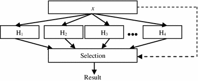
Classifier selection
-
(B)
Classifier fusion Here, the outputs of many different classifiers are mixed instead of extracting a single best classifier. Each classifier in the ensemble has some knowledge of the entire feature space and tries to solve the same classification problem using different methods based on different training sets, classifiers or parameters. The final output is determined by fusing the decisions of the individual classifiers as shown in Fig. 2. All classifiers in the ensemble are trained over the entire feature space.
Fig. 2 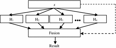
Classifier fusion


2.2 Existing methods
Several methods have been developed for the construction of ensembles. Some methods are general and they can be applied to any learning algorithm, whereas others are specific to particular algorithms. Next, we report some of the basic approaches for the construction of ensembles.
-
(A)
Different classifier models For effectiveness we can use several types of learning algorithms from different backgrounds, e.g., decision tree, neural network, nearest neighbor, etc. However, we can use the same classifier with a slight change in the user-defined parameters, leading to significant variation in classification results.
-
(B)
Different feature subsets Classifiers are built using different subsets of features of the training dataset. It works only when some redundancy in features is present on the training dataset. Both the deterministic and random approaches can be used for selecting different feature subsets of input data. In the deterministic approach, a prior knowledge about the input data is required, whereas the random approach uses random subspace method for selecting the different feature subsets. Here, each classifier is selected on a random space, and a feature in the subset is selected with a probabilistic approach. Random forests, which uses decision trees, is an example of this method. However, a common problem with this random method is that some subspaces lack information and as a result may not give good performance.
-
(C)
Different training sets One learning algorithm is run on different random sub-samples of training data to produce different classifiers. It works well for unstable learners, i.e., output classifier undergoes major changes, given only small changes in training data. Random sub-samples of the training data can be generated using re-sampling and re-weighing. Bagging and wagging use re-sampling, while Boosting and ARCing uses re-weighing of the training dataset.
-
(D)
Different combination schemes Different classifiers are trained on the training data and their outputs are combined using different combination schemes like majority voting, algebraic combiners, etc., to get the final output. Next we discuss the basics of various combination methods and their effectiveness.
2.3 Ensemble combination method
An ensemble of classifiers can be trained simply on different subsets of the training data, different parameters of the classifiers, or even with different subsets of features as in random subspace models. The classifiers can then be combined using one of the combination rules. Some of these combination rules operate on class labels only, whereas others need continuous outputs that can be interpreted as support given by the classifier to each of the classes. Xu et al. (1992) define three types of base model outputs to be used for classifier combination.
-
(a)
Abstract-level output, where each classifier outputs a unique class label for each input pattern.
-
(b)
Rank-level output, where each classifier outputs a list of ranked class labels for each input pattern.
-
(c)
Measurement-level output, where each classifier outputs a vector of continuous-valued measures that can represent estimates of class posterior probabilities or class-related confidence values that represent the support for the possible classification hypotheses.
Figure 3 shows different types of ensemble combination methods and subsequently describes each of them briefly.

Ensemble combination methods
2.3.1 Combining class labels
If the outputs of the combined classifiers are in the form of class labels, then they can be combined using any of the following methods (Polikar 2008).
-
1.
Majority voting In this approach, each classifier has equal vote and the most popular classification is the one chosen by the ensemble as a whole (Polikar 2008). The most basic variant is the plurality vote, where the class with the most votes wins. In general, we have three versions of majority voting as given below.
-
(a)
One on which all classifiers agree (unanimous voting).
-
(b)
Predicted by at least one more than half the number of classifiers (simple majority).
-
(c)
One that receives the highest number of votes, whether or not the sum of those votes exceeds 50 % (plurality voting or just majority voting).
However, none of these versions is free from the common limitations of majority voting.
-
2.
Weighted majority voting If we have evidence that certain experts are more qualified than others, weighing the decisions of those qualified experts more heavily may further improve the overall performance. Let us denote the decision of hypothesis h t on class c j as d t,j such that d t,j is 1 if h t selects c j and 0 otherwise. Further, we assume that the classifiers are assigned weights according to their performances such that classifier h t is assigned weight w t .
The total weights received by a class is the sum of the product of the weights of the classifiers, w t and their respective decisions, d t,j . The class receiving the highest weighted vote is selected as the final decision of the ensemble. Thus, according to this assumption, an ensemble will select class J if the following holds:
2.3.2 Combining continuous outputs
Continuous output is interpreted as the degree of support given to a class by a classifier, usually accepted as the value of the posterior probability for that class (Polikar 2008). Algebraic combiners are used to merge the decisions of the classifiers in continuous output format, following the convention as given above:
-
(A)
Sum rule The total support for a class is calculated as the sum of the supports given to that class by all the classifiers. After calculating the total supports for all the classes, the class with the highest support is selected as the final output.
$$\mu_{j} \left( x \right) = \sum\limits_{t = 1}^{T} {d_{t,j} (x)} $$(1) -
(B)
Mean rule This rule is similar to the sum rule but the total support is normalized by 1/T (T = number of classifiers).
$$\mu_{j} \left( x \right) = \frac{1}{T}\sum\limits_{t = 1}^{T} {d_{t,j} (x)} $$(2) -
(C)
Weighted sum rule By this rule, the support for a class is calculated by the sum of the product of the classifiers’ weight and their respective supports.
$$\mu_{j} \left( x \right) = \sum\limits_{t = 1}^{T} {w_{t} d_{t,j} (x)} $$(3) -
(D)
Product rule Here, supports provided by the classifiers to a particular class are multiplied to obtain the final support for that class. This rule is very sensitive to the pessimistic classifiers as a low support can remove any chance of getting selected by that class.
$$\mu_{j} \left( x \right) = \prod\limits_{t = 1}^{T} {d_{t,j} (x)} $$(4) -
(E)
Maximum rule As the name suggests, this rule selects the maximum of all the supports of the different classifiers for a particular class.
$$\mu_{j} \left( x \right) = { \hbox{max} }_{t = 1}^{T} \{ d_{t,j} \left( x \right)\} $$(5) -
(F)
Minimum rule This rule selects the minimum of all the supports of the different classifiers for a particular class.
$$\mu_{j} \left( x \right) = { \hbox{min} }_{t = 1}^{T} \{ d_{t,j} \left( x \right)\} $$(6) -
(G)
Median rule This rule selects the median of the supports of the different classifiers for a particular class.
$$\mu_{j} \left( x \right) = {\text{median}}_{t = 1}^{T} \{ d_{t,j} \left( x \right)\} $$(7) -
(H)
Generalized mean rule Many of the above rules are in fact special cases of the generalized mean rule which is as follows:
$$\mu_{j, \propto } \left( x \right) = \left[ {\frac{1}{T}\sum\limits_{t = 1}^{T} {d_{t,j} (x)^{ \propto } } } \right]^{{\frac{1}{ \propto }}} $$(8)
The methods of combination described above are summarized in Table 1.
2.3.3 Other combination rules
Few other combination rules not listed above are (Polikar 2008): (i) Borda count: takes the rankings of the class supports into consideration; (ii) behavior knowledge space: lists the most common correct classes in a lookup table for all probable class combinations given by the classifiers; (iii) decision templates: computes a similarity measure between the current decision profile of the unknown instance and the average decision profiles of instances from each class; and (iv) Dempster–Schafer rule: computes the plausibility based belief measures for each class.
2.4 Discussion
Based on our empirical study on these various combination methods, it has been observed that:
-
Most classifiers are application dependent and inconsistent in performance over majority of datasets.
-
An ensemble method with an appropriate set of base classifiers is found to perform better than the individual classifiers.
-
Appropriate training samples can improve the performance of the classifiers significantly.
-
Performance of the majority of combination methods is affected by the presence of outliers.
-
The sum rule or the weighted majority voting gives good results.
-
A significant improvement in classification accuracy becomes possible with a meta-ensemble, i.e., ensemble of ensembles, if the base ensemble methods perform consistently well and the combination method is carefully selected.
3 Related work
In the past decade, many researchers have devoted their efforts to the study of ensemble decision tree methods for microarray classification. Ensemble decision tree methods combine decision trees generated from multiple training datasets by re-sampling the training dataset. Bagging, Boosting and Stacking are some of the well-known ensemble methods in the machine learning field.
We have selected three classifiers, i.e., J48 (decision tree), IBK (instance-based learner) and Naive Bayes (probabilistic) as the base classifiers based on the following grounds:
-
All these classifiers performed consistently well over several real-life UCI datasets.
-
They are from three different classification algorithms families.
-
They belong to three different states, i.e., stable, unstable and probabilistic.
In this section, we highlight the classifiers and the ensembles used in our study.
3.1 Base classifiers
3.1.1 J48
Decision tree J48 implements Quinlan’s C4.5 algorithm (Quinlan 1993) for generating a pruned or unpruned C4.5 tree. Decision trees are built from a set of labeled training data using the concept of information entropy. Based on each attribute of the data, a decision can be arrived at by splitting the data into smaller subsets.
J48 examines the normalized information gain (difference in entropy) that results from choosing an attribute for splitting the data. To arrive at a decision, the attribute with the highest normalized information gain is used. Then the algorithm recursively moves on to the smaller subsets and the splitting procedure stops if all instances in a subset belong to the same class. Next, a leaf node is created in the decision tree indicating the class. In case none of the features give any information gain, then J48 creates a decision node higher up in the tree using the expected value of the class.
J48 can handle both continuous and discrete attributes, training data with missing attribute values and attributes with differing costs. It also provides an option for pruning trees after creation.
3.1.2 IBk
Instance-based classifiers (Aha et al. 1991) such as the kNN classifier operate on the assumption that classification of unknown instances can be done by relating the unknown to the known based on some distance/similarity function. The probability of two instances far apart in the instance space (as defined by the appropriate distance function) belonging to the same class is less likely than two closely situated instances.
The algorithm computes the k closest neighbors of an instance of an unknown class and the class is assigned by voting among those neighbors. To prevent ties, the value of k is taken as an odd number for binary classification. Plurality voting or majority voting is used for multiple classes but the latter can sometimes result in no class being assigned to an instance, while the former can result in classifications being made with very low support from the neighborhood. Another option is to weigh each neighbor by an inverse function of its distance to the instance being classified.
3.1.3 Naïve Bayes (NB)
Naïve Bayes classifier (John and Langley 1995) is a probabilistic classifier based on the Bayes theorem assuming a strong (Naïve) independence of attributes. Naïve Bayes classifiers take into consideration that all attributes (features) independently contribute to the probability of a certain decision. It analyzes independently all the attributes of the data with equal importance and hence Naïve Bayes classifiers can be trained very efficiently in a supervised learning setting.
3.2 Ensemble methods
3.2.1 Bagging
Bagging (Breiman 1996a) is an ensemble method where the same learning algorithm is used for different training datasets to obtain different classifiers. The diversity amongst the training datasets is achieved by a bootstrap technique used to re-sample the training dataset. As shown in Fig. 4, each classifier is then trained on a re-sample of instances, which then assigns a predicted class to this set of instances. The individual classifiers’ predictions (having equal weightage) are then combined by taking majority voting.

Block diagram of multiple classifier systems based on Bagging. D i class prediction by the ith classifier
3.2.2 Boosting
Boosting (Freund and Schapire 1996) uses a re-sampling technique different from Bagging. In this case, a new training dataset is generated according to its sample distribution. The first classifier is constructed from the original dataset where every sample has an equal weight (Fig. 5). In the succeeding training dataset, the weight is reduced if the sample has been correctly classified, otherwise it is increased if the samples are misclassified. In the committee decision, a weighted voting method is used so that a more accurate classifier is given greater weightage than a less accurate classifier.

Block diagram of multiple classifier systems based on Boosting. D i class prediction by the ith classifier
3.2.3 Stacked generalization
Stacked generalization (or stacking), proposed by Wolpert (1992), performs its task in two phases (Fig. 6): (i) the layer-1 base classifiers are trained using bootstrapped samples of the level-0 training dataset and (ii) the outputs of layer-1 are then used to train a layer-2 meta-classifier. The purpose is to check whether the training data have been properly learned. For example, if a particular classifier incorrectly learns a certain region of the feature space and hence consistently misclassifies instances coming from that region, then the level-2 classifier may be able to learn this behavior, and along with the learned behaviors of other classifiers, and correct such improper training. Polikar (2008) proposed to use class probabilities rather than class labels as the output in the level-1 dataset, so as to improve the stacking performance.

Multiple classifiers based on stack generalization
3.3 Discussion
-
(i)
The selection of the base classifiers has been done based on the fact that they are diverse in nature and have been established over the 2 class problems.
-
(ii)
To eliminate the biasness of individual classifiers, the ensemble method is adopted so that the overall classification accuracy is improved and also the errors of one classifier are averaged out by the correct classification of another classifier.
-
(iii)
Bagging and Boosting of each of the base classifiers is done so as to derive the maximum benefit in terms of classification accuracy.
-
(iv)
The individual ensemble approaches are also not totally free from their limitations, so an approach of creating an ensemble of ensembles (Dettling 2004) is found to be suitable to maximize classification accuracy.
3.4 Motivation for a new ensemble method
Based on our limited experimental study, it has been observed that:
-
Algorithms from different classification families can be used with appropriate combination method to form an effective ensemble.
-
To reduce error rates, it is a necessary condition to combine the relatively uncorrelated output predictions. With highly correlated output predictions, there is little scope for the reduction in error, as the committee of experts has no diversity to draw from.
-
A strong reason for combining models across different algorithm families can be stated as—different algorithms will provide uncorrelated output estimates because of their varied classification functions.
-
Abbott (1994) showed considerable differences in classifier performance class by class—information that is clear, once classifier is obscure to another. Since it is difficult to know a priori which algorithm(s) will produce the lowest error for each domain (on unseen data), combining models across algorithm families mitigates that risk by including contributions from all the families.
The motivation is to devise a cost-effective ensemble method, SD-EnClass, not influenced by the biasness of the base classifiers and which shows consistently improved detection rates compared to the base classifiers in the combination (Table 2).
4 Experimental design methodology
Tenfold cross-validation is used in this experiment where the dataset is partitioned into ten sets of equal size. Nine of these sets are combined and used for training, while the remaining one is used for testing. Then the process is repeated with nine different sets combined for training and so on until all the ten individual partitions have been used for testing. The final accuracy of an algorithm will be the average of the ten trials. The datasets were obtained from Kent Ridge Biological Dataset Repository (Li and Liu 2002). Table 3 shows the summary of the characteristics of the nine datasets. The experiments were conducted on varying proportions of the training and test datasets and also conducted using tenfold cross-validation on the merged original training and test data. The proportion of the training data was consistently kept below 60 %. Since determining how much data is needed for training and testing is one of the key issues of data mining, we have worked around this issue using varying proportions of training and test datasets to avoid over-fitting, without compromising on accuracy. The performances shown in Table 5 are an average of the experiments using varying proportions of the training and test datasets and tenfold cross-validation on the merged original training and test data.
4.1 Software used for comparison
All the algorithms were executed in WEKA (Weka 3.6.2) package which is available online (http://www.cs.waikato.ac.nz/ml/weka/) with their default parameter settings in a high-end workstation with 3.33 GHz Intel Xeon processor and 8 GB RAM and the proposed model was implemented in the same environment using Java (jdk1.6). Default settings are used for all compared ensemble methods as they showed a high accuracy on an average.
5 The proposed SD-EnClass
Our model for combining classifiers into an ensemble is based on a simple estimation of each classifier’s expertise (accuracy) on class prediction. This technique is a simple combining method which can use any ‘n’ stronger learners as base classifiers to build an effective ensemble. Predictions of the ‘n’ classifiers are combined to obtain the best prediction for a given test instance. In our experimental setup, we choose decision trees, Bayesian classifier and k-nearest neighbor learners as the base learners based on their consistent performance over real-life datasets such as UCI.
Our model utilizes the expertise of a classifier in classifying a part of the problem better than the other classifiers in the ensemble. It explores the necessary property of the diversity among the base classifiers to have a good performing ensemble. It is known that different classifiers handle the problem of classification at hand differently. So an attempt has been made to combine the results of such diverse classifiers to obtain a better classification result than using a single classifier alone.
The architecture of the proposed model is shown in Fig. 7. It is a two-layer model, where each layer is dedicated with a definite functionality. The output of the layer-1 is used as input by the layer-2. Layer-1 deals with the training and selection of the base classifiers, while layer-2 deals with the combination of the predictions of the selected base classifiers.

Architecture of the proposed SD-EnClass
5.1 Distinct training sample selection
The proposed SD-EnClass uses a 2-step technique, referred as SD-Prune-Redundant, to select a distinct subset of training samples by discarding the redundant training instances. This forms the input to the tenfold cross-validation. Since the performance of classifiers is dependent on its training, so effort is made to create a training set which is complete in nature, i.e., the training set should hold instances that would represent the entire domain space. Steps of SD-Prune-Redundant are given next.
-
1.
Convert training dataset D Train into market–basket form D MB using Algorithm 1 (Fig. 8a);
-
2.
Filter D MB using Algorithm 2 to remove duplicate training instances (Fig. 8b).
5.2 Working of the SD-EnClass
Initially, the base classifiers are trained with the distinct training dataset. Next, we evaluate the performance of the base classifiers using the test dataset. The classifier with the highest class performance for a certain class out of the base classifiers becomes the expert of that class. The class-specific performance of a classifier is calculated as:
To evaluate the class performance of a classifier, a confusion matrix as shown in Table 4 is used. The elements in this table characterize the classification behavior of a given classifier. The sum of the row elements represents the number of total instances present in each class, whereas the sum of the column elements gives the total number of instances predicted as that class.

a Market–basket conversion, b distinct training instance selection
As shown in Table 4, the total number of instances present for class A is (x + p + l), and the total number of instances predicted for class A is (x + y + z). Here, we have taken three classes in the table, for more number of classes, the rows and columns will increase, respectively.
Example: Let the total number of predicted instances for class A be 100, and total number of correctly predicted instances for class A is 90, then the class-specific accuracy (CSA) for class A for that classifier is 90/100, i.e., 0.9.
We compute the CSA for each base classifier for each class and accuracy values are stored using a 2-D link list structure. For our experimental setup, we choose three (n = 3) base classifiers. In the link list structure, the nodes in the rows correspond to the number of base classifiers in the ensemble and the column nodes correspond to the number of classes in the dataset. From this data structure, the class expert for a given class is easily found. During classification of an instance, the instance is first classified by the base classifiers and the individual predictions of the base classifiers are combined as follows:
-
1.
For a given instance, if all the classifiers predict the same class, then the ensemble goes by the same decision.
-
2.
If the predictions of majority classifiers (2 of 3) match, then any of the following situations may arise:
-
(a)
C3 is an expert in the class it predicts whereas C1 and C2 are not, then the prediction given by C3 is taken as the decision of the ensemble.
-
(b)
C3 is an expert in the class it predicts and anyone of the classifiers, C1 and C2, is also an expert in its predictions then the ensemble looks for the class probabilities of the respective classifiers and selects the one with the highest value. If there exists a further tie between the probability values then the ensemble goes with the majority.
-
3.
If the predictions of all the classifiers disagree, then any of the following situations may arise:
-
(a)
One of the classifiers could be an expert in its prediction then the ensemble goes by that classifier’s decision.
-
(b)
Two classifiers could be experts in its class predictions. In such a case, the decision of the classifier which has a higher class probability is taken as the final decision.
-
(c)
All the three classifiers could be experts in its class predictions. In that case, the decision of the classifier which has the highest class probability is taken as the final decision.
In this manner, the class predictions of the base classifiers are combined to get the final prediction.
5.3 Performance analysis of our proposed model
In this phase, we test the performance of our proposed model. We combine the outputs of J48, IBK and Naïve Bayes classifiers with the combination rule we proposed earlier and the results are depicted in Table 5.
From Table 5 and graph in Fig. 9, it is clear that our proposed model has been successful in increasing the prediction accuracy in 4 of 9 datasets while in 2 datasets it has been at par with the best performing classifier. Thus, in 6 [i.e., (4 + 2)] datasets, the proposed model has shown a good performance, whereas in 4 datasets the performance has decreased. Nonetheless, the proposed model has been successful in more than 60 % of the cases.

Performance analysis of the proposed model
Next, we apply the three basic ensemble approaches, i.e., Bagging, Boosting and Stacking, for each of the base classifiers and analyze their performance. For Stack Generalization, we used the three classifiers as the base learners and use these three classifiers as Meta-learners one by one and compare their performances. We notice that Bagging, Boosting and Stacking improved the performance of J48 and NB, while Stacking with IBK slightly improved the performance of IBK at the expense of computation time. This is because Bagging and Boosting mainly improve the performances of unstable learners; being a stable learner, IBKs’ performance was not affected much.
While comparing our proposed model with the existing ensembles, we see from Table 6 and Fig. 10 that the proposed model has not been able to outperform the existing ensembles in most of the cases. The prediction accuracy is slightly less than the best performing ensemble.

Performance analysis of the proposed model with existing ensembles
Notably, the new model is able to have the highest accuracy in 1 dataset; in 2 datasets, it is at par with the best existing ensemble and in 3 datasets it has been the second best performer. To sum up, it cannot be concluded that the proposed model has been the best performer, but it has shown an average performance. To improve the prediction accuracy further, we have thus proposed the meta-ensemble.
6 Meta-ensemble
From the results of the previous section, it is clear that combining the outputs of different classifiers improves classification accuracy than the best single classifier in the combination, but it does not perform as well as boosting. The advantage of boosting acts directly to reduce the error cases, whereas combining works indirectly. As our proposed model works well to get the best output from the combination, we used this method to combine the results of our ensemble with the results of boosting, stacking and bagging and form a meta-ensemble; the architecture is shown in Fig. 11.

Architecture of the meta-ensemble
The new meta-ensemble is a four-layer model where each layer has a definite functionality and the output of the lower layers is used by the higher layers. More summarized results are presented while traversing toward the higher layers.
In layer-1, any n classifier models are generated. Here n could be any integer, but in our case n is set to 3. Layer-1 could be further improved by training a larger number of classifier models and selecting a small set of good performing classifier models out of them. That would definitely increase the overall accuracy of the proposed model.
Layer-2 is the ensemble layer where the individual outputs of the consistent base classifiers are combined as described in Sect. 5.2. The output of the ensemble is stored in a file which is then fed in layer-4.
Layer-3 creates a pool of classifier ensembles. Popular methods such as Bagging, Boosting and Stack Generalization (Stacking) are implemented with the classifier models which are selected in layer-1 and their performances recorded. Stacking is implemented with the three classifiers as base learners and taking one of them at a time as a meta-learner. Two best performing ensembles are selected for layer-4 along with the proposed ensemble model.
Layer-4 finally combines the output of layer-2 and layer-4, i.e., our ensemble model and the two best performing ensembles from layer-3 to give the final prediction.
A comparative analysis of the meta-ensemble with the existing ensembles is presented in Table 7. For each of the datasets, Boosting, Bagging and Stacking performed differently. We combined the outputs of the two best performing methods out of boosting, bagging and stacking for each of the classifiers with the result given by our proposed model.
The results of Table 7 are summarized in Fig. 12. We observe that of the 9 datasets, our method works well for 8 of them, while performing average in one of the datasets. Of the 8 datasets it performed well, it improved classification accuracy in 4 of them significantly, while in remaining 4 it performed as well as the best classifier in the combination.

Performance analysis of the meta-ensemble
Thereby we can say from the above results that given a set of classifiers our proposed model combines the prediction of the classifiers to obtain a better prediction result which in most of the cases is better than selecting the best classifier in the combination of classifiers.
7 Conclusion and future work
In this paper, we analyze the performances of popular ensemble methods like Bagging, Boosting and Stack Generalization. We found out that on an average, Boosting and Stack Generalization using unstable learners (decision trees) and probabilistic classifiers (Naïve Bayes) work better than applying them to stable learners (nearest neighbor classifiers). We also learnt that Bagging of classifiers performs better than Boosting and Stack Generalization for most of the cancer datasets used in our experiments.
We have also proposed an effective way of combining the outputs of the classifiers in the ensemble, based on the class performance of each of the classifiers in the combination. The experimental results show that our model performs better than making a simple selection of the best single classifier in the combination in majority of the cases. In doing so, we mostly tested our model on two class datasets for which it performed well; we also tested on one multi-class dataset on which we got good performance and in future we can extend the combination rules so that it works even better for multi-class problem.
While combining models across the different algorithm families, we saw an improvement of performance in the classification accuracy compared to the best single model in the combination, but when compared to Bagging, its performance was average. So in the next stage, we combined the results of our proposed ensemble with the results of the best performing ensemble methods for the datasets, using our proposed combining method and obtained results which were significantly better than using Boosting, Bagging or Stacking alone.
In the modern era where computing technologies are getting better every day, we can use our method in parallelization to achieve better classification accuracy to solve a classification problem. There is scope to incorporate self-computing approaches (like fuzzy, roughset, ANN or their hybridization) in the proposed model for further enhancement of performance.
References
Abbott DW (1994) Comparison of data analysis and classification algorithms for automatic target recognition. In: Proceedings of the 1994 IEEE International Conference on Systems, Man and Cybernetics, San Antonio
Aha DW, Kibler D, Albert MK (1991) Instance-based learning algorithms. Mach Learn 6:37–66
Ahmed H, Mahanta P, Bhattacharyya DK, Kalita JK (2011) Gerc: tree based clustering for gene expression data. In: 2011 IEEE 11th international conference on Bioinformatics and Bioengineering (BIBE), IEEE, New York, pp 299–302
Ahmed H, Mahanta P, Bhattacharyya DK, Kalita JK (2012) Module extraction from subspace co-expression networks. Netw Model Anal Health Inf Bioinformatics 1(4):183–195
Boström H, Johansson R, Karlsson (2008) A on evidential combination rules for ensemble classifiers. In: Proceedings of the 11th International Conference on Information Fusion
Breiman L (1996a) Arcing classifiers. Technical Report 486, Statistics Department, University of California, Berkeley, CA. 94720
Breiman L (1996b) Bagging predictors. Mach Learn 24(2):123–140
Dettling M (2004) BagBoosting for tumor classification with gene expression data. Bioinformatics 20(18):3583–3593
Dietterich T (1997) Machine-learning research: four current directions. AI Magazine 18(4):97–136
Dietterich TG (2000) An experimental comparison of three methods for constructing ensembles of decision trees: bagging, boosting, and randomization. Mach Learn 40:139–157
Elder JF IV, Pregibon D (1996) A statistical perspective on knowledge discovery in databases. In: Fayyad U, Piatetsky-Shapiro G, Smyth P (eds) Advances in knowledge discovery and data mining. AAAI Press, Menlo Park, pp 83–113
Freund Y, Schapire R (1996) Experiments with a new boosting algorithm. In: Proceedings of 13th international conference on machine. Learn Bari, Italy, pp 148–156
Jiang D, Tang C, Zhang A (2004) Cluster analysis for gene expression data: a survey. IEEE Trans Knowl Data Eng 16(11):1370–1386
John GH, Langley P (1995) Estimating continuous distributions in bayesian classifiers. In: Proceedings of the eleventh conference on uncertainty in artificial intelligence, pp 338–345
Kiliç C, Tan M (2012) Positive unlabeled learning for deriving protein interaction networks. Netw Model Anal Health Inf Bioinformatics 1(3):87–102
Kuncheva LI (2001) Combining classifiers: soft computing solutions. In: Pal SK, Pal A (eds) Pattern recognition: from classical to modern approaches. World Scientific Publishing Co., Singapore, pp 427–452
Li J, Liu H (2002) Kent ridge bio-medical dataset repository. http://levis.tongji.edu.cn/gzli/data/mirror-kentridge.html
Lockhart D, Dong H, Byrne M et al (1996) Expression monitoring by hybridization to high-density oligonucleotide arrays. Nat Biotechnol 14:1675–1680
Mahanta P, Ahmed H, Bhattacharyya DK, Kalita J (2011) Triclustering in gene expression data analysis: a selected survey. In: Proceedings of the 2nd national conference on emerging trends and applications in computer science (NCETACS). doi:10.1109/NCETACS.2011.5751409
Nagi S, Bhattacharyya DK, Kalita J (2011a) Gene expression data clustering: a survey. In: Proceedings of the 2nd national conference on emerging trends and applications in computer science (NCETACS). doi:10.1109/NCETACS.2011.5751377
Nagi S, Bhattacharyya DK, Kalita JK (2011b) Subspace clustering in gene expression data analysis: a survey. In: Sharma U, Nath B, Bhattacharyya DK (eds) Machine intelligence: recent advances, Narosa Publishing, Delhi, pp 211-219, March 2011, ISBN 978-81-8487-140-1
Polikar R (2008) Ensemble learning. Scholarpedia 4(1):2776. http://www.scholarpedia.org/article/Ensemble_learning
Quinlan JR. (1993) C4.5: programs for machine learning. Morgan Kaufmann, San Mateo
Schadt E, Li C, Ellis B, Wong W (2001) Feature extraction and normalization algorithms for high-density oligonucleotide gene expression array data. J Cellular Biochem 84(S37):120–125
Schena M, Shalon R, Davis D, Brown P (1995) Quantitative monitoring of gene expression patterns with a complementary DNA microarray. Science 270:467–470
Steinberg D, Colla P (1997) CART-classification and regression trees. Salford Systems, San Diego
Tan AC, Gibert D (2003) Ensemble machine learning on gene expression data for cancer classification. Appl Bioinformatics 2(3):s75–s83
Van Hulse J, Khoshgoftaar TM, Napolitano A, Wald R (2012) Threshold-based feature selection techniques for high-dimensional bioinformatics data. Netw Model Anal Health Inf Bioinformatics 1(1–2):47–61
Wolpert DH (1992) Stacked generalization. Neural Netw 5:241–259
Xu L, Krzyzak A, Suen CY (1992) Methods for combining multiple classifiers and their applications to handwriting recognition. IEEE Trans Syst Man Cybernetics 22(3):418–435
Author information
Authors and Affiliations
Corresponding author
Rights and permissions
About this article
Cite this article
Nagi, S., Bhattacharyya, D.K. Classification of microarray cancer data using ensemble approach. Netw Model Anal Health Inform Bioinforma 2, 159–173 (2013). https://doi.org/10.1007/s13721-013-0034-x
Received:
Revised:
Accepted:
Published:
Issue Date:
DOI: https://doi.org/10.1007/s13721-013-0034-x