Non-Gaussian Covariate-Dependent Spatial Measurement Error Model for Analyzing Big Spatial Data

Abstract

Spatial models based on the Gaussian distribution have been widely used in environmental sciences. However, real data could be highly non-Gaussian and may show heavy tails features. Moreover, as in any type of statistical models, in spatial statistical models, it is commonly assumed that the covariates are observed without errors. Nonetheless, for various reasons such as measurement techniques or instruments used, measurement error (ME) can be present in the covariates of interest. This article concentrates on modeling heavy-tailed geostatistical data using a more flexible class of ME models. One novelty of this article is to allow the spatial covariance structure to depend on ME. For this purpose, we adopt a Bayesian modeling approach and utilize Markov chain Monte Carlo techniques and data augmentations to carry out the inference. However, when the number of observations is large, statistical inference is computationally burdensome, since the covariance matrix needs to be inverted at each iteration. As another novelty, we use a prediction-oriented Bayesian site selection scheme to tackle this difficulty. The proposed approach is illustrated with a simulation study and an application to nitrate concentration data. Supplementary materials accompanying this paper appear online.

Appendices

Appendix

A Spatial Data Decorrelation

Let , and assume the parameters ${\varvec{\mu }},\theta$ and $\delta ^2$ are known. Then, . This decorrelated vector can now be used for assessing normality. However, in practice, as the parameters are unknown, they are replaced by some appropriate estimates. The details are as follows: (I) Estimate ${\varvec{\mu }}$ using ordinary least squares; (II) estimate the covariance parameters $\theta$ and $\delta ^2$ based on the variogram of ; (III) calculate the Cholesky decomposition $LL'$ of , and (IV) decorrelate the data as .

B Proofs

This section presents some detailed proofs of the results shown in Sect. 2.1. To prove Eq. (4), let $Y_\mathbf{w}\left( {s} \right) ={Y\left( {s} \right) } \left| {{\mathbf{w}}\left( {s} \right) } \right.$ and follow the definition and simple properties of the covariance (and variance) as:

(10)

(11)

Let . The proof of Eq. (6) requires calculating the following terms:

$$\begin{aligned} \mathrm{Kurt}\left[ Y_\mathbf{w}\left( {s} \right) \right]= & {} \frac{{E\left[ {{{\left( {{Y_{\mathbf{w}}}\left( s \right) - E\left[ {{Y_{\mathbf{w}}}\left( s \right) } \right] } \right) }^4}} \right] }}{{{{\left\{ {\mathrm{Var}\left[ {{Y_{\mathbf{w}}}\left( s \right) } \right] } \right\} }^2}}}\nonumber \\= & {} \frac{{E\left[ {{Y_{\mathbf{w}}}{{\left( s \right) }^4}} \right] - 4{{\varvec{\mu }}_s}E\left[ {{Y_{\mathbf{w}}}{{\left( s \right) }^3}} \right] + 6{\varvec{\mu }}_s^2E\left[ {{Y_{\mathbf{w}}}{{\left( s \right) }^2}} \right] - 3{\varvec{\mu }}_s^4}}{{{{\left[ {\sigma ^2}\exp \left\{ {\nu } \right\} +{\sigma _u^2{{\varvec{\beta }}_x'} {{\varvec{\beta }}_x}}{+\tau ^2 }\right] }^2}}}. \end{aligned}$$

(12)

In what follows, we compute each of the expected values in the above equation separately (details not presented here).

Thus, substituting these expectations in (12), the marginal kurtosis is reduced to (6). Ultimately, we focus on Eq. (7).

(13)

Palacios and Steel (2006) showed that in the absence of a nugget effect,

$$\begin{aligned} E\left[ {{{\left( {\sigma \frac{{\varepsilon \left( s \right) }}{{\sqrt{\lambda \left( s \right) } }}} \right) }^n}} \right] = \left\{ \begin{array}{ll} 0&{}\text {for } n \text { odd,}\\ {\sigma ^n}{c_n}\exp \left\{ {\frac{{n\nu }}{4}\left( {1 + \frac{n}{2}} \right) } \right\} &{}\text {for }n \text {even,} \end{array} \right. \end{aligned}$$

(14)

and on the other hand,

$$\begin{aligned} E\left[ {{{\left( { - {\mathbf{u'}}\left( s \right) {{\varvec{\beta }}_x}} \right) }^n}} \right] = \left\{ \begin{array}{ll} 0&{}\text {for } n \text { odd,}\\ \frac{{{{\left( {\sigma _u^2{{\varvec{\beta }}_x'}{{\varvec{\beta }}_x}} \right) }^{\frac{n}{2}}}}}{{{2^{\frac{n}{2}}}}}\frac{{n!}}{{\left( {\frac{n}{2}} \right) !}} &{}\text {for } n \text { even;} \end{array} \right. \end{aligned}$$

(15)

hence, Eq. (7) can be easily obtained by substituting (14) and (15) into (13).

C Prediction-Oriented Site Selection

Determining${\mathbf{s}}^\pi$: We choose the nearest sites to the prediction sites ${{{\mathbf{s}}^p}}$ in q-tier, where q determines ${n_\pi }$ as ${n_\pi } = q{n_p}$ and can be derived through an examination of the fitting to ${{\mathbf{Y}}\left( {{{\mathbf{s}}^\pi }} \right) }$ or its subset (e.g., one can choose the value of ${n_\pi }$ such that the mean squared fitting errors for the first-tier neighboring sites are minimized among a few values of ${n_\pi }$ under consideration). The selection scheme entails the following steps:

1.:

For $i = 1, \ldots , n_p$, do the following sub-steps to identify the first tier of the nearest sites to ${{{\mathbf{s}}^p}}$:

(a):

Draw a site $s_i^p$ from the set ${{{\mathbf{s}}^p}}$ at random and without replacement.

(b):

Identify the nearest neighbor of $s_i^p$ by setting $s_{1,i}^\pi = \mathop {arg\min }\limits _{s \in {\mathbf{s}}\backslash \left\{ {s_{1,1}^\pi , \ldots ,s_{1,i - 1}^\pi } \right\} } \left\| {s - s_i^p} \right\|$ and finally, set ${\mathbf{s}}_1^\pi = \left\{ {s_{1,1}^\pi , \ldots ,s_{1,{n_p}}^\pi } \right\}$.

2.:

Set ${\mathbf{s}} \leftarrow {\mathbf{s}}\backslash {\mathbf{s}}_1^\pi$ and repeat the sub-steps in step 1 to identify the second tier of the nearest sites to ${{{\mathbf{s}}^p}}$. Denote the second-tier neighboring set by ${\mathbf{s}}_2^\pi$.

$\vdots$

q.:

Set ${\mathbf{s}} \leftarrow {\mathbf{s}}\backslash {\mathbf{s}}_{q-1}^\pi$ and repeat the sub-steps in step 1 to identify the qth tier of the nearest sites to ${{{\mathbf{s}}^p}}$. Denote the qth tier neighboring set by ${\mathbf{s}}_q^\pi$.

This procedure provides ${{\mathbf{s}}^\pi } = \bigcup \nolimits _{r = 1}^q {{\mathbf{s}}_r^\pi }$ as the set of response variables.

Determining${\mathbf{s}}^{\delta }$: We aim to draw ${n_\delta }$ sites from the set ${\mathbf{s}}\backslash {{\mathbf{s}}^\pi }$. To minimize the loss of data information caused by site selection, ${\mathbf{s}}^\delta$ should be selected uniformly from the observation region of ${\left\{ {Y\left( {{s_i}} \right) } \right\} }$ and thus, following the theory of Poisson process, the number of selected sites can be modeled as a Poisson random variable. Therefore, to enhance our selection pattern, we impose a truncated Poisson prior distribution as $\pi \left( {n_\delta } \right) \propto \left( {{{c_0}^{n_\delta }}}/{{{n_\delta }!}}\right) \exp \left\{ { - {{c_0}}} \right\}$, ${n_\delta } = 0,1, \ldots ,{n_d} - {n_\pi }$, where ${c_0}$ is a hyper-parameter which have to be specified by the user. Alternatively, one can specify a prior distribution that incorporates the spatial information of ${\mathbf{Y}}\left( {{{\mathbf{s}}^{-\pi }}} \right)$, but this will complicate the simulation of the posterior distribution.

D Bayesian Posterior Sampling

In this section, we summarize the Gibbs sampling iterates for drawing samples from the posterior $P\left( {{\varvec{\lambda }},{\mathbf{W}},{{\varvec{\varepsilon }}},{{\varvec{\eta }}},{{\mathbf{Y}^\delta }}\left| {{{\mathbf{y}}^\pi }} \right. } \right)$. So, we need to specify all full conditional distributions (which are presented in Sect. D.1). However, the difficulty associated with drawing samples from the full conditional distribution of ${{\mathbf{Y}^\delta }}$ is that a direct application of MCMC fails as it requires the state space of the Markov chain to be of a fixed dimension, but the dimension of ${{\mathbf{Y}^\delta }}$ may actually vary. To overcome this issue, we can use a reversible-jump MCMC (RJMCMC) algorithm (Green 1995), which allows the dimension of the state space of the Markov chain to vary. The underlying idea is that RJMCMC introduces three types of moves: exchange, birth and death. Exchange means that the chain remains in the space with the same dimension, but moves into a new state. Birth and death are the moves that change the dimension of the state space. Intuitively, a birth step augments the state space by adding new states, whereas a death step reduces the dimension of the state space. At each iteration, the type of move, whether an exchange, birth, or death, is randomly chosen with the respective proposal probabilities denoted by $q_e$, $q_b$ and $q_d$, and one accepts the new state using a Metropolis–Hastings rule.

Let ${\left\{ {{{\varvec{\lambda }}^{\left( t \right) }},{{\mathbf{W}}^{\left( t \right) }},{{{\varvec{\varepsilon }}}^{\left( t \right) }},{{{\varvec{\eta }}}^{\left( t \right) }},{ {{\mathbf{y}^\delta }}^{\left( t \right) }}} \right\} }$ denote the sample generated at the iteration t. Obviously, $min\left( {n_\delta }\right) =0$ and $max\left( {n_\delta }\right) =n_d - n_\pi$. To update ${{\mathbf{y}^\delta }}^{\left( t \right) }$, we use a RJMCMC move. For ${n_\delta }=0$, we consider $q_e={1}/{3}$ and $q_b={2}/{3}$; for ${n_\delta }=n_d - n_\pi$, we set $q_e={1}/{3}$ and $q_d={2}/{3}$; and finally for ${n_\delta }= 1, \ldots ,{n_d} - {n_\pi } - 1$, we suppose $q_b = q_d = q_e ={1}/{3}$. Given ${{{\varvec{\lambda }}^{\left( t \right) }},{{\mathbf{W}}^{\left( t \right) }},{{{\varvec{\varepsilon }}}^{\left( t \right) }},{{{\varvec{\eta }}}^{\left( t \right) }},{ {{\mathbf{y}^\delta }}^{\left( t \right) }}}$, the next iteration of the Gibbs sampler consists of the following steps: (I) Generate ${{\varvec{\lambda }}^{\left( t+1 \right) }},{{\mathbf{W}}^{\left( t+1 \right) }},{{{\varvec{\varepsilon }}}^{\left( t+1 \right) }}$ and ${{{\varvec{\eta }}}^{\left( t+1 \right) }}$ from their corresponding full conditional distributions. (II) Draw ${ {{\mathbf{y}^\delta }}^{\left( t+1 \right) }}$:

• (Birth) Uniformly randomly choose a point from ${{\varvec{D}}}_{-\pi }\backslash { {{\mathbf{y}^\delta }}^{\left( t \right) }}$, say ${y}^*$, and add it to the current site set ${{\mathbf{y}^\delta }}^{\left( t \right) }$ (i.e., ${{{\mathbf{y}^\delta }}^{\left( {t + 1} \right) }} = {{{\mathbf{y}^\delta }}^{\left( t \right) }} \cup { {y}^*}$) with probability

  $$\begin{aligned} \min \left\{ {1,\frac{{P\left( {{{\varvec{\lambda }}^{\left( {t + 1} \right) }},{{\mathbf{W}}^{\left( {t + 1} \right) }},{{{\varvec{\varepsilon }}}^{\left( {t + 1} \right) }},{{{\varvec{\eta }}}^{\left( {t + 1} \right) }}\left| {{{\mathbf{y}}^\pi },{{ {y}}^*}} \right. } \right) P \left( {{{{ {y}}}^*}} \right) }}{{P\left( {{{\varvec{\lambda }}^{\left( t \right) }},{{\mathbf{W}}^{\left( t \right) }},{{{\varvec{\varepsilon }}}^{\left( t \right) }},{{{\varvec{\eta }}}^{\left( t \right) }}\left| {{{\mathbf{y}}^\pi },{ {{\mathbf{y}^\delta }}^{\left( t \right) }}} \right. } \right) P \left( {{ {{\mathbf{y}^\delta }}^{\left( t \right) }}} \right) }}\frac{{{n_d} - {n_\pi } - {n_\delta } }}{{{n_\delta } + 1}}\frac{{{q_d}}}{{{q_b}}}} \right\} . \end{aligned}$$

• (Death) Uniformly randomly select ${y}^*$ out of ${ {{\mathbf{y}^\delta }}^{\left( {t } \right) }}$ and remove it from the current site set ${ {{\mathbf{y}^\delta }}^{\left( t \right) }}$ (i.e., ${{{\mathbf{y}^\delta }}^{\left( {t + 1} \right) }} = {{{\mathbf{y}^\delta }}^{\left( t \right) }}\backslash { {y}^*}$) with probability

  $$\begin{aligned} \min \left\{ {1,\frac{{P\left( {{{\varvec{\lambda }}^{\left( {t + 1} \right) }},{{\mathbf{W}}^{\left( {t + 1} \right) }},{{{\varvec{\varepsilon }}}^{\left( {t + 1} \right) }},{{{\varvec{\eta }}}^{\left( {t + 1} \right) }}\left| {{{\mathbf{y}}^\pi },{{ {y}}^*}} \right. } \right) P \left( {{{ {y}}^*}} \right) }}{{P\left( {{{\varvec{\lambda }}^{\left( t \right) }},{{\mathbf{W}}^{\left( t \right) }},{{{\varvec{\varepsilon }}}^{\left( t \right) }},{{{\varvec{\eta }}}^{\left( t \right) }}\left| {{{\mathbf{y}}^\pi },{{{\mathbf{y}^\delta }}^{\left( t \right) }}} \right. } \right) P\left( {{{{\mathbf{y}^\delta }}^{\left( t \right) }}} \right) }}\frac{{{n_\delta }}}{{{{n_d}-{n_\pi }-{n_\delta } } + 1}}\frac{{{q_b}}}{{{q_d}}}} \right\} . \end{aligned}$$

• (Exchange) Uniformly randomly choose ${y}^*$ from ${{\varvec{D}}}_{-\pi }\backslash {{{\mathbf{y}^\delta }}^{\left( t \right) }}$ and also ${y}^{**}$ from ${{{\mathbf{y}^\delta }}^{\left( {t} \right) }}$. Then, exchange ${y}^*$ and ${y}^{**}$ (i.e., ${{{\mathbf{y}^\delta }}^{\left( {t + 1} \right) }} = {{{\mathbf{y}^\delta }}^{\left( t \right) }} \cup \left\{ {{ {y}^*}} \right\} \backslash \left\{ {{ {y}^{**}}} \right\}$) with probability

  $$\begin{aligned} \min \left\{ {1,\frac{{P\left( {{{\varvec{\lambda }}^{\left( {t + 1} \right) }},{{\mathbf{W}}^{\left( {t + 1} \right) }},{{{\varvec{\varepsilon }}}^{\left( {t + 1} \right) }},{{{\varvec{\eta }}}^{\left( {t + 1} \right) }}\left| {{{\mathbf{y}}^\pi },{{ {y}}^*}} \right. } \right) }}{{P\left( {{{\varvec{\lambda }}^{\left( t \right) }},{{\mathbf{W}}^{\left( t \right) }},{{{\varvec{\varepsilon }}}^{\left( t \right) }},{{{\varvec{\eta }}}^{\left( t \right) }}\left| {{{\mathbf{y}}^\pi },{ {\mathbf{y}^\delta }^{\left( t \right) }}} \right. } \right) }}} \right\} . \end{aligned}$$

1.1 D.1 The Full Conditional Distributions

Below, we describe the full conditional distributions of all unobservable quantities through a Gibbs sampler framework to draw samples from $P\left( {{\varvec{\lambda }},{\mathbf{W}},{{\varvec{\varepsilon }}},{{\varvec{\eta }}}\left| {{{\mathbf{y}}^\pi }, {{\mathbf{y}^\delta }}} \right. } \right)$. In what follows, we use the notation ${{ \textit{g} _{ - \vartheta }}}$ to show the vector $\textit{g}$ without $\vartheta$. Moreover, we partition the latent variables into two parts as follows: ${\varvec{\lambda }}= \left( {{{\varvec{\lambda }}^\pi }',{{\varvec{\lambda }}^\delta }'} \right) '$, ${{\varvec{\varepsilon }}}= \left( {{{{\varvec{\varepsilon }}}^\pi }',{{{\varvec{\varepsilon }}}^\delta }'} \right) '$, ${\mathbf{W}} = \left( {{{\mathbf{W}}^\pi },{{\mathbf{W}}^\delta }} \right)$ and $\Lambda = \left( {{\Lambda ^\pi },{\Lambda ^\delta }} \right)$, respective to the location sets ${\mathbf{s}}^\pi$ and ${{{\mathbf{s}}^\delta }}$. Regardless of the details, the full conditional distributions are as follows:

• Latent variable${{\varvec{\psi }}}$: For each of the components of ${{\varvec{\psi }}}^\pi$ (i.e., ${\psi _i}$), we can write

  

  (16)

where the first term in the right-hand side of (16), i.e., the likelihood contribution, is proportional to a product of normal density functions truncated on $\left[ 0,\infty \right)$. To construct a suitable candidate generator, we approximate this distribution by log-normal distributions on $\lambda _i$s. By matching the first two moments of $\lambda _i$, we obtain an approximating distribution of the likelihood contribution to $\psi _i$ as

$$\begin{aligned} N\left( {{a_i},b_i^2} \right) ,\qquad {a_i} = \ln \frac{\sigma ^2{\varepsilon _i^2\left[ {1 + {h_i}\ell \left( {{h_i}} \right) + h_i^2} \right] }}{{\left[ {\sigma _u^2{{\varvec{\beta }}_x'} {{\varvec{\beta }}_x} {+\tau ^2}} \right] {{\left[ {\ell \left( {{h_i}} \right) + {h_i}} \right] }^4}}},\qquad b_i^2 = 4\ln \frac{{1 + {h_i}\ell \left( {{h_i}} \right) + h_i^2}}{{{{\left[ {\ell \left( {{h_i}} \right) + {h_i}} \right] }^2}}},\nonumber \\ \end{aligned}$$

(17)

such that ${h_i} = {{{\sigma }{{{t}}_{{1_i}}}sign\left( {{\varepsilon _i}} \right) }}/{\sqrt{\sigma _u^2{{\varvec{\beta }}_x'} {{\varvec{\beta }}_x}{+\tau ^2}} }$, ${{\mathbf{t}}_1} = \sigma ^{-1}\left( {{{\mathbf{y}}^\pi } - {\beta _0}{{\mathbf{1}}_{{n_\pi }}} - {{\mathbf{W}}^\pi }{{\varvec{\beta }}_x}} \right)$, ${sign\left( {\cdot } \right) }$ denotes the sign function and ${\ell \left( \cdot \right) } = {{\phi \left( \cdot \right) }}/{{\Phi \left( \cdot \right) }}$ where $\phi$ and $\Phi$ denote the standard normal density and cumulative distribution function, respectively. On the other hand, the second term in the right-hand side of (16) can be easily obtained as

(18)

where ${\Sigma {{ ^{\left( i \right) }}^\prime }}$ shows the ith row of ${{\Sigma }}$ and ${\Sigma ^{\left( { - i, - i} \right) }}$ is ${{\Sigma }}$ in which the ith row and the ith column have been omitted. Combining (18) and (17), we propose a candidate value for $\psi _i$, say $\psi _i^{cand}$ from ${\psi _i}\left| {{{\mathbf{y}}^\pi }, {{\mathbf{y}^\delta }},{{{\varvec{\psi }}}_{ - i}^\pi },{{{\varvec{\psi }}}^\delta },{\mathbf{W}},{{\varvec{\varepsilon }}},{{\varvec{\eta }}}} \right. \sim N\left( {\frac{{b_i^2a_i^* + b_i^{{*^2}}{a_i}}}{{b_i^2 + b_i^{{*^2}}}},\frac{{b_i^2b_i^{{*^2}}}}{{b_i^2 + b_i^{{*^2}}}}} \right)$ where $a_i^*$ and $b_i^{{*^2}}$ are the mean and the variance of the normal distribution in (18), respectively.

• Latent variable$\mathbf W$: Suppose that ${{\mathbf{t}}_2} = \left( {{{\mathbf{y}}^\pi } - {\beta _0}{{\mathbf{1}}_{{n_\pi }}} - \sigma {{{{{\varvec{\varepsilon }}}^\pi }}}/{{\sqrt{{{\varvec{\lambda }}^\pi }} }}} \right)$. Then,

  

  (19)

At iteration t, the coefficient vector ${\varvec{\beta }}$ is known and so a sample from ${{\mathbf{W}}^\pi }\left| {{{\mathbf{y}}^\pi },{{\mathbf{y}^\delta }},{\varvec{\lambda }},{{\mathbf{W}}^\delta },{{\varvec{\varepsilon }}},{{\varvec{\eta }}}} \right.$ can be easily obtained as a solution of the under-determined systems of linear equations $\mathbf{W}^\pi {\varvec{\beta }}_x=\mathscr {C}$, where $\mathscr {C}$ is a sample of (19). If the under-determined linear system has no solution, $\mathscr {C}$ is substituted with another sample of (19).

• Latent variable${{\varvec{\varepsilon }}}$: Let ${{t}_{{1_i}}^*}={t_{{1_i}}}\sqrt{{\lambda _i^\pi }}$ for $i=1,2,\ldots ,n_\pi$, $\textit{g} _\varepsilon = {\Sigma _{\pi \delta }}\Sigma _\delta ^{ - 1}{{{\varvec{\varepsilon }}}^\delta }$ and $\mathcal {G}_\varepsilon ={\Sigma _\pi } - {\Sigma _{\pi \delta }}\Sigma _\delta ^{ - 1}{\Sigma _{\delta \pi }}$. Thus, for $A_1{ = [{{{\sigma ^2}}}/\left( {\sigma _u^2{{\varvec{\beta }}_x'} {{\varvec{\beta }}_x}}{+\tau ^2}\right) ]{\Lambda ^{{\pi ^{ - 1}}}} + \mathcal{G}_\varepsilon ^{ - 1}}$,

  $$\begin{aligned} {{{{\varvec{\varepsilon }}}^\pi }\left| {{{\mathbf{y}}^\pi }, {\mathbf{y}^\delta },{\varvec{\lambda }},{\mathbf{W}},{{{\varvec{\varepsilon }}}^\delta },{{\varvec{\eta }}}} \right. }\sim {N_{n_\pi }}\left( {{A_1^{ - 1}\left[ {{\Lambda ^{{\pi ^{ - 1}}}}{\mathbf{t}}_1^* + \mathcal{G}_\varepsilon ^{ - 1}{g_\varepsilon }} \right] },A_1^{ - 1}} \right) . \end{aligned}$$

• The intercept: By setting ${{\mathbf{t}}_3} = {{\mathbf{y}}^\pi } - {\mathrm{{W}}^\pi }{{\varvec{\beta }}_x} - \sigma {{{{{\varvec{\varepsilon }}}^\pi }}}/{\sqrt{{{\varvec{\lambda }}^\pi }} }$, the conditional distribution of the intercept parameter is obtained as

  $$\begin{aligned} N\left( {\left[ {{\frac{{{n_\pi }}}{{ {\sigma _u^2{{\varvec{\beta }}_x'} {{\varvec{\beta }}_x}{+\tau ^2}}}} + \frac{1}{{{c_1}}}}}\right] ^{-1}{{\sum \limits _{i = 1}^{{n_\pi }} {{t_{{3_i}}}} }}/{{ \left( {\sigma _u^2{{\varvec{\beta }}_x'} {{\varvec{\beta }}_x}{+\tau ^2}}\right) }},\left[ {{\frac{{{n_\pi }}}{{{\sigma _u^2{{\varvec{\beta }}_x'} {{\varvec{\beta }}_x}{+\tau ^2}} }} + \frac{1}{{{c_1}}}}}\right] ^{-1}} \right) . \end{aligned}$$

In the six last items, the full conditional distribution of parameters ${\varvec{\beta }}_x$, $\sigma ^2$, $\tau ^2$, $\nu$, $\theta _1$ and $\theta _2$ are of nonstandard forms, so a Metropolis–Hastings step or a sampling importance resampling (SIR) algorithm can be used. Choosing the first approach to draw samples from an unknown quantity, say $\vartheta$, consists of accepting the produced value $\vartheta ^*$ from the candidate generator $q\left( {\vartheta ^*} \right)$ at the kth iteration with probability $min\left\{ 1,r_k\right\}$, where ${r_k} = {{f\left( {{\vartheta ^*}\left| {data} \right. } \right) q\left( \vartheta ^{\left( k \right) } \right) }}/{{f\left( {{\vartheta ^{\left( k \right) }}\left| {data} \right. } \right) q\left( {{\vartheta ^*}} \right) }}$ and $f\left( {{\cdot }\left| data \right. } \right)$ is proportional to the posterior distribution of $\vartheta$. By choosing the SIR algorithm, we may generate (say m) approximate samples from the posterior distribution of $\vartheta$ as follows:

• Draw samples $\left\{ {{\vartheta ^{\left( i \right) }}} \right\} _{i = 1}^m$ from the proposal distribution $q\left( \vartheta \right)$,

• Calculate importance weights ${\omega _i} = {f\left( {{\vartheta ^{\left( i \right) }}\left| data \right. }\right) /{q\left( {{\vartheta ^{\left( i \right) }}} \right) }}$,

• Normalize the importance weights as ${p_i} = {{{\omega _i}}/ {\sum \nolimits _i {{\omega _i}} }}$,

• Resample with replacement from $\left\{ {{\vartheta ^{\left( i \right) }}} \right\} _{i = 1}^L$ with sample probabilities $p_i$.

A conservative candidate distribution for applying the SIR algorithm is the pre-specified prior on $\vartheta$.

• Parameter${\varvec{\beta }}_x$: It is easy to see that $\pi \left( {{{\varvec{\beta }}_x}\left| {{{\mathbf{y}}^\pi }, {\mathbf{y}^\delta },{\varvec{\lambda }},{\mathbf{W}},{{\varvec{\varepsilon }}},{{{\varvec{\eta }}}_{ - {{\varvec{\beta }}_x}}}} \right. } \right)$ is proportional to

  $$\begin{aligned} {\left( {\frac{1}{{{{{\varvec{\beta }}}_x'}{{\varvec{\beta }}_x}}}} \right) ^{\frac{n_\pi }{2}}}\exp \left\{ { - \frac{1}{{2{c_1}}}{{{\varvec{\beta }}}_x'}{{\varvec{\beta }}_x}} \right\} \exp \left\{ { - \frac{1}{2\left( {\sigma _u^2}{{\varvec{\beta }}_x'}{{\varvec{\beta }}_x}{+\tau ^2}\right) }{{\left( {{\mathbf{t}_2} - {\mathbf{W} ^\pi }{{\varvec{\beta }}_x}} \right) }^\prime }\left( {{\mathbf{t}_2} - {\mathbf{W} ^\pi }{{\varvec{\beta }}_x}} \right) } \right\} , \end{aligned}$$

and the proposal distribution ${N_k}\left( {{{\mathbf{W}}^\pi }^\prime {{\mathbf{t}}_2},\left[ {{c_1} + \sigma _u^2} {+\tau ^2}\right] {I_k}} \right)$ is of interest.

• Parameter$\sigma ^2$: Similarly, for ${{\mathbf{t}}_4} = {{\mathbf{y}}^\pi } - {\beta _0}{{\mathbf{1}}_{{n_\pi }}} - {{\mathbf{W}}^\pi }{{\varvec{\beta }}_x}$, $\pi \left( {{\sigma ^2}\left| {{{\mathbf{y}}^\pi },{\mathbf{y}^\delta },{\varvec{\lambda }},{\mathbf{W}},{{\varvec{\varepsilon }}},{{{\varvec{\eta }}}_{ - {\sigma ^2}}}} \right. } \right)$ is proportional to

  $$\begin{aligned} {\left( {\sigma ^2} \right) ^{ - \frac{n_\pi }{2} - 1}}\exp \left\{ { - \frac{1}{2}\left[ {\frac{{c_2^2}}{{\sigma ^2}} + c_3^2{\sigma ^2}} \right] } \right\} \exp \left\{ { - \frac{1}{{2\left( {\sigma _u^2}{{\varvec{\beta }}_x'}{{\varvec{\beta }}_x}{+\tau ^2}\right) }}\sum \limits _{i = 1}^{n_\pi } {{{\left( {{t_{{4_i}}} - \sigma \frac{{{\varepsilon _i^\pi }}}{{\sqrt{{\lambda _i^\pi }} }}} \right) }^2}} } \right\} , \end{aligned}$$

and our suggested proposal distribution is $GIG\left( {{{{n_\pi }}}/{2},{c_2},\sqrt{c_3^2 + \sum \nolimits _{i = 1}^{{n_\pi }} {{{\varepsilon _i^\pi }}/{{\sqrt{\lambda _i^\pi } }}} } } \right)$.

• Parameter$\tau ^2$: $\pi \left( {\tau ^2\left| {{{\mathbf{y}}^\pi },{{\mathbf{y}}^\delta },{\varvec{\lambda }},{\mathbf{W}},{{\varvec{\varepsilon }}},{{{\varvec{\eta }}}_{ - \tau ^2}}} \right. } \right)$ is a proportion of

$$\begin{aligned} {\left( {\tau ^2} \right) ^{ - \frac{n_\pi }{2} - 1}}\exp \left\{ { - \frac{1}{2}\left[ {\frac{{c_4^2}}{{\tau ^2}} + c_5^2{\tau ^2}} \right] } \right\} \exp \left\{ { - \frac{1}{{2\left( {\sigma _u^2}{{{\varvec{\beta }}}_x'}{{\varvec{\beta }}_x}+\tau ^2\right) }}\sum \limits _{i = 1}^{n_\pi } {t_{5_i}^2} } \right\} \end{aligned}$$

where ${{\mathbf{t}}_5} = {{\mathbf{y}}^\pi } - {\beta _0}{{\mathbf{1}}_{{n_\pi }}} - {{\mathbf{W}}^\pi }{{\varvec{\beta }}_x} - \sigma {{{{{\varvec{\varepsilon }}}^\pi }}}/{{\sqrt{{{\varvec{\lambda }}^\pi }} }}$.

• Parameter$\nu$: Consider ${ \textit{g} _\lambda } = - \left( {\nu }/{2}\right) {{\mathbf{1}}_{{n_\pi }}} + {\Sigma _{\pi \delta }}\Sigma _\delta ^{ - 1}\left( {{\ln {\varvec{\lambda }}^\delta } + \left( {\nu }/{2}\right) {{\mathbf{1}}_{{n_d} - {n_\pi }}}} \right)$ and ${\mathcal {G}_\lambda } = {\Sigma _\pi } - {\Sigma _{\pi \delta }}\Sigma _\delta ^{ - 1}{\Sigma _{\delta \pi }}$. Then, ${\nu \left| {{{\mathbf{y}}^\pi },{\mathbf{y}^\delta },{\varvec{\lambda }},{\mathbf{W}},{{\varvec{\varepsilon }}},{{{\varvec{\eta }}}_{-\nu } }} \right. }$ is a proportion of

$$\begin{aligned} \exp \left\{ { - \frac{1}{{2\nu }}{{\left( {\ln {\varvec{\lambda }}^\pi -{ \textit{g} _\lambda }} \right) }^\prime }{\mathcal {G}_\lambda ^{- 1}}\left( {\ln {\varvec{\lambda }}^\pi - { \textit{g} _\lambda }} \right) } \right\} \frac{1}{{{\nu ^{\frac{n_\pi }{2} + 1}}}}\exp \left\{ { - \frac{1}{2}\left[ {\frac{{c_6^2}}{\nu } + c_7^2\nu } \right] } \right\} \end{aligned}$$

and so a candidate distribution can be chosen as

$$\begin{aligned} GIG\left( {\frac{{{n_\pi }}}{2},{{\left[ {c_6^2 + {{\left( {\ln {{\varvec{\lambda }}^\pi } - {\Sigma _{\pi \delta }}\Sigma _\delta ^{ - 1}\ln {{\varvec{\lambda }}^\delta }} \right) }^\prime }G_\lambda ^{ - 1}\left( {\ln {{\varvec{\lambda }}^\pi } - {\Sigma _{\pi \delta }}\Sigma _\delta ^{ - 1}\ln {{\varvec{\lambda }}^\delta }} \right) } \right] }^{\frac{1}{2}}},{c_7}} \right) . \end{aligned}$$

• Parameter$\theta _1$: Similarly, $\pi \left( {{\theta _1}\left| {{{\mathbf{y}}^\pi }, {\mathbf{y}^\delta },{\varvec{\lambda }},{\mathbf{W}},{{\varvec{\varepsilon }}},{{{\varvec{\eta }}}_{ - {\theta _1}}}} \right. } \right)$ is proportional to

  

A conservative candidate distribution is the pre-specified prior on $\theta _1$.

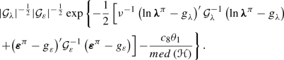
• Parameter$\theta _2$: Finally, $\pi \left( {{\theta _2}\left| {{{\mathbf{y}}^\pi }, {\mathbf{y}^\delta },{\varvec{\lambda }},{\mathbf{W}},{{\varvec{\varepsilon }}},{{{\varvec{\eta }}}_{ - {\theta _2}}}} \right. } \right)$ is a proportion of

  $$\begin{aligned} {\left| {\mathcal {G}_\lambda } \right| ^{ - \frac{1}{2}}}{\left| {\mathcal {G}_\varepsilon } \right| ^{ - \frac{1}{2}}}\exp \left\{ - \frac{1}{{2 }}\left[ \nu ^{-1}\left( {\ln {\varvec{\lambda }}^\pi -{ \textit{g} _\lambda }} \right) ^\prime {\mathcal {G}_\lambda ^{- 1}}\left( {\ln {\varvec{\lambda }}^\pi - { \textit{g} _\lambda }} \right) { + {{\left( {{{{\varvec{\varepsilon }}}^\pi } - { \textit{g} _\varepsilon }} \right) }^\prime }\mathcal{G}_\varepsilon ^{ - 1}\left( {{{{\varvec{\varepsilon }}}^\pi } - {g_\varepsilon }} \right) } \right] \right\} , \end{aligned}$$

  and again we choose the pre-specified prior on $\theta _2$ as the proposal distribution.

References

S.E. Alexeeff, R.J. Carroll, and B. Coull. Spatial measurement error and correction by spatial SIMEX in linear regression models when using predicted air pollution exposures. Biostatistics, 17(2):377–389, 2016.
R. Bastian and D. Murray. Guidelines for water reuse. US EPA Office of Research and Development, Washington, DC, EPA/600/R-12/618, 2012.
R.S. Bueno, T.C.O. Fonseca, and A.M. Schmidt. Accounting for covariate information in the scale component of spatio-temporal mixing models. Spatial Statistics, 22:196–218, 2017.
E.K. Choi and Y.P. Kim. Effects of aerosol hygroscopicity on fine particle mass concentration and light extinction coefficient at Seoul and Gosan in Korea. Asian Journal of Atmospheric Environment, 4(1):55–61, 2010.
T.C.O Fonseca and M.F.J. Steel. Non-Gaussian spatio-temporal modelling through scale mixing. Biometrika, 98(4):761–774, 2011.
W.A. Fuller. Measurement Error Models. John Wiley & Sons, 2009.
A. Gelman and D.B. Rubin. Inference from iterative simulation using multiple sequences. Statistical Science, pages 457–472, 1992.
P.J. Green. Reversible jump markov chain monte carlo computation and Bayesian model determination. Biometrika, 82(4):711–732, 1995.
R. Haining. Spatial Data Analysis in the Social and Environmental Sciences. Cambridge University Press, 1993.
M.J. Heaton, A. Datta, A. Finley, R. Furrer, R. Guhaniyogi, F. Gerber, R.B. Gramacy, D. Hammerling, M. Katzfuss, F. Lindgren, et al. Methods for analyzing large spatial data: A review and comparison. arXiv preprint arXiv:1710.05013, 2017.
M.H. Huque, H.D. Bondell, and L. Ryan. On the impact of covariate measurement error on spatial regression modelling. Environmetrics, 25(8):560–570, 2014.
M.H. Huque, H.D. Bondell, R.J. Carroll, and L.M. Ryan. Spatial regression with covariate measurement error: A semiparametric approach. Biometrics, 72(3):678–686, 2016.
R. Ingebrigtsen, F. Lindgren, and I. Steinsland. Spatial models with explanatory variables in the dependence structure. Spatial Statistics, 8:20–38, 2014.
J.C. Jarvis, M.G. Hastings, E.J. Steig, and S.A. Kunasek. Isotopic ratios in gas-phase HNO\(_3\) and snow nitrate at Summit, Greenland. Journal of Geophysical Research: Atmospheres, 114(D17):1–14, 2009.
H.M. Kim and B.K. Mallick. A Bayesian prediction using the skew Gaussian distribution. Journal of Statistical Planning and Inference, 120(1-2):85–101, 2004.
Y. Li, H. Tang, and X. Lin. Spatial linear mixed models with covariate measurement errors. Statistica Sinica, 19(3):1077, 2009.
J.H. V. Neto, A.M. Schmidt, and P. Guttorp. Accounting for spatially varying directional effects in spatial covariance structures. Journal of the Royal Statistical Society: Series C (Applied Statistics), 63(1):103–122, 2014.
B.T. Nolan and J.D. Stoner. Nutrients in groundwaters of the conterminous United States, 1992- 1995. Environmental Science & Technology, 34(7):1156–1165, 2000.
S.P. Opsahl, M. Musgrove, and R.N. Slattery. New insights into nitrate dynamics in a karst groundwater system gained from in situ high-frequency optical sensor measurements. Journal of hydrology, 546:179–188, 2017.
M.B. Palacios and M.F.J. Steel. Non-Gaussian Bayesian geostatistical modeling. Journal of the American Statistical Association, 101(474):604–618, 2006.
J. Park and F. Liang. A prediction-oriented Bayesian site selection approach for large spatial data. Journal of Statistical Research, 47(1):11–30, 2015.
B.J. Reich, J. Eidsvik, M. Guindani, A.J. Nail, and A.M. Schmidt. A class of covariate-dependent spatio-temporal covariance functions for the analysis of daily ozone concentration. The Annals of Applied Statistics, 5(4):2265, 2011.
A. Sathasivan, I. Fisher, and T. Tam. Onset of severe nitrification in mildly nitrifying chloraminated bulk waters and its relation to biostability. Water research, 42(14):3623–3632, 2008.
A.M. Schmidt, P. Guttorp, and A. O’Hagan. Considering covariates in the covariance structure of spatial processes. Environmetrics, 22(4):487–500, 2011.
M.F.J Steel and M. Fuentes. Non-Gaussian and non-parametric models for continuous spatial data. Handbook of Spatial Statistics, pages 149–167, 2010.
V. Tadayon. Bayesian analysis of censored spatial data based on a non-gaussian model. Journal of Statistical Research of Iran, 13(2):155–180, 2017.
Acknowledgements
The Associate Editor and two referees are gratefully acknowledged. Their precise comments and constructive suggestions have clearly improved the manuscript.
Author information
Authors and Affiliations
Corresponding author
Electronic supplementary material
Below is the link to the electronic supplementary material.
Supplementary Materials
The supplementary materials contain R codes and corresponding “ReadMe” files for the simulation and real data application conducted in this paper. (zip 69 KB)