Robust computation tree logic

Abstract

It is widely accepted that every system should be robust in that “small” violations of environment assumptions should lead to “small” violations of system guarantees, but it is less clear how to make this intuition mathematically precise. While significant efforts have been devoted to providing notions of robustness for linear temporal logic, branching-time logics, such as computation tree logic (CTL) and CTL*, have received less attention in this regard. To address this shortcoming, we develop “robust” extensions of CTL and CTL*, which we name robust CTL (rCTL) and robust CTL* (rCTL*). Both extensions are syntactically similar to their parent logics but employ multi-valued semantics to distinguish between “large” and “small” violations of the specification. We show that the multi-valued semantics of rCTL make it more expressive than CTL, while rCTL* is as expressive as CTL*. Moreover, we show that the model checking problem, the satisfiability problem, and the synthesis problem for rCTL and rCTL* have the same asymptotic complexity as their non-robust counterparts, implying that robustness can be added to branching-time logics for free.

1 Introduction

Specifications for reactive systems are typically written as an implication $\Phi \Rightarrow \Psi$ where $\Phi$ is an environment assumption and $\Psi$ is a system guarantee. However, the specification $\Phi \Rightarrow \Psi$ is even satisfied if the environment assumption $\Phi$ is violated, no matter how the system behaves. This behavior is clearly inadequate since the environment assumptions will inevitably be violated in the real world: the actual environment where the system will be deployed is often not entirely known at design time and, thus, cannot be accurately and entirely formalized by the formula $\Phi$.

There have been concentrated efforts in the literature to prevent reactive systems from behaving arbitrarily when the environment assumption is violated, typically by making the specifications robust to violations of the environment assumption. For instance, Bloem et al. [1], Tarraf et al. [2], Doyen et al. [3], Ehlers et al. [4], and Tabuada et al. [5, 6] have provided different ways of introducing robustness for specifications in linear temporal logic (LTL). All these approaches require additional assumptions or quantitative information from the designer, which is often tedious and hard to obtain.

This drawback has motivated Tabuada and Neider [7] to introduce a new logic, named robust LTL (rLTL), which provides robustness without relying on any additional assumptions or input from a designer beyond an LTL formula. Among rLTL’s main features are its ease of use (one simply “dots” temporal operators in existing LTL formulas) and the fact that adding robustness does not change the asymptotic complexity of the model checking, runtime monitoring, and synthesis problems [7,8,9,10,11,12,13,14,15]. Inspired by this logic, there have been several works introducing robust extensions of different classes of temporal logics [8, 9, 16, 17].¹

In this work, we investigate robust branching-time logics. Such logics, like Computation Tree Logic (CTL) and CTL*, have received less attention in this regard. A notable exception is the work of French et al. [18, 19], which introduces logics called RoCTL and RoCTL*. However, this logic again uses operators that require a manual quantification of the violations of the environment assumptions.

To address this shortcoming, we develop robust extensions of CTL and CTL*, which we call robust CTL (rCTL) and robust CTL* (rCTL*), which are inspired by the notion of robustness in rLTL. Similar to rLTL, our new logics employ multi-valued semantics to track the degree of violations of a specification and are guided by two objectives. First, the syntax of rCTL and rCTL* is similar to CTL and CTL*, respectively. Second, the notion of robustness in these logics is intrinsic rather than extrinsic, i.e., robustness does not rely on the designers to provide quantitative information about the specification, such as the number of violations permitted, ranks, cost, etc.

As a demonstration of how our notion of robustness works, consider a specification $\Phi \Rightarrow \Psi$ for a robot deployed in an office-like environment. The environment assumption states that the human workers in the office never visit the robot’s dock. On the other hand, the robot guarantee states: “for all trajectories, regardless of the robot’s current position, the robot can return to its dock in one time step” (note that such a specification cannot be expressed in LTL). Ideally, we would then want the following:

• if the office workers satisfy the assumption $\Phi$, then the robot should also satisfy the guarantee $\Psi$;

• if the office workers violate the assumption by visiting the dock a finite number of times before realizing their mistake and eventually not visiting it anymore, i.e., if they only satisfy , then the robot should also satisfy , i.e., the robot eventually should be able to return to its dock from any point; and

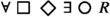• if the office workers violate the assumption by visiting the dock infinitely often (or eventually always), i.e., if they satisfy (or ), then the robot should satisfy (or , respectively).

We later show that the semantics of rCTL and rCTL* indeed captures such a notion of robustness.

The first two contributions of the paper are robust variants of the logics CTL and CTL*, namely rCTL (in Sect. 3) and rCTL* (in Sect. 5), respectively. Their semantics rely on many-valued truth values that capture the various degrees of how a specification can be violated.

After having introduced rCTL and rCTL*, we study their expressive power and compare them to existing logics such as LTL, rLTL, CTL, and CTL* (in Sects. 3.3 and 5.3). Our key results are that rCTL is more expressive than CTL, while rCTL* has the same expressive power as CTL*.

Next, we provide efficient model-checking algorithms for rCTL and rCTL* to demonstrate that both logics can be effectively used for verification. We establish that the rCTL model checking problem is $\textrm{PTIME}$-complete (in Sect. 3.4) and that the rCTL* model checking problem is $\textrm{PSPACE}$-complete (in Sect. 5.4). Note that this is the same asymptotic complexity as CTL and CTL* model checking, respectively. Moreover, we show that the satisfiability and reactive synthesis problems for rCTL (in Sects. 3.6 and 3.7) and rCTL* (in Sects. 5.5 and 5.6) match the exact asymptotic complexity of their non-robust counterparts, i.e., $\textrm{EXPTIME}$-completeness for rCTL and $\textrm{2EXPTIME}$-completeness for rCTL*. Thus, robustness can be added to branching-time logics “for free”. Table 1 shows an overview over our complexity results.

Table 1 Summary of our results (in bold) and comparison to other logics

This paper is an extension of a conference paper [20]. The new content includes all proofs missing from the conference paper, an example illustrating our rCTL model-checking procedure, more details about the embedding of rCTL and rCTL* into the modal $\mu$-calculus, and the investigation of the rCTL and rCTL* synthesis problems.

2 Notation and review of computation tree logic

In this section, we review the syntax and semantics of CTL, which expresses properties of Kripke structures.

Throughout this paper, we fix a finite set $\mathcal {P}$ of atomic propositions. A Kripke structure $M = (S,I,R,L)$ over $\mathcal {P}$ consists of a set of states S, a set of initial states $I\subseteq S$, a transition relation $R\subseteq S\times S$ such that for all states s there exists a state $s'$ satisfying $(s,s')\in R$, and a labeling function $L:S\rightarrow 2^{\mathcal {P}}$. We say that M is finite if it has finitely many states. In that case, we define the size of M as $|S|$.

The set $\textrm{post}(s) = \{s'\in S \mid (s,s') \in R\}$ contains all successors of $s \in S$. A path of the Kripke structure M is an infinite sequence $\pi = s_0s_1\cdots$ of states such that $s_{i+1} \in \textrm{post}(s_i)$ for each $i\ge 0$. For a state s, let $\textrm{paths}(s)$ denote the set of all paths starting from s. Furthermore, for a path $\pi$ and $i\ge 0$, let $\pi [i]$ denote the i-th state of $\pi$, and let $\pi [i..]$ denote the suffix of $\pi$ from index i on.

2.1 Syntax

CTL formulas are classified into state and path formulas. Intuitively, state formulas express properties of states, whereas path formulas express temporal properties of paths. For ease of notation, we denote state formulas and path formulas by Greek capital letters and Greek lowercase letters, respectively. CTL state formulas over $\mathcal {P}$ are given by the grammar

$$\begin{aligned} \Phi {:}{:}=p \mid \Phi \vee \Phi \mid \Phi \wedge \Phi \mid \lnot \Phi \mid \Phi \Rightarrow \Phi \mid \exists \varphi \mid \forall \varphi , \end{aligned}$$

where $p\in \mathcal {P}$ and $\varphi$ is a path formula. CTL path formulas are given by the grammar

where , and denote the operators next, eventually, always, until, and weak until, respectively. Note that we include implication, conjunction (alternatively, disjunction), and weak until as part of the syntax, instead of derived operators. We do this to be consistent with the syntax of robust logics, where these operators can no longer be derived. As we will see later, it is also instructive to include the operators eventually and always explicitly.

2.2 Semantics

Slightly deviating from the usual approach, we define the CTL semantics using a mapping $V_{\text {CTL}}$ that maps a state/path and a CTL formula to a truth value in $\mathbb {B} = \{0,1\}$. Also, some of our definitions are non-standard in order to be closer to the robust semantics introduced later. However, let us stress that the definition below is equivalent to the usual semantics of CTL (see, e.g., Baier and Katoen [21]).

Given a state s and state formulas $\Phi ,\Psi$, CTL semantics is defined as follows:

$$\begin{aligned} V_{\text {CTL}}(s,p)&= {\left\{ \begin{array}{ll} 0 &{} \text {if }p\not \in L(s); \text { and} \\ 1 &{} \text {if }p\in L(s), \\ \end{array}\right. }\\ V_{\text {CTL}}(s,\Phi \vee \Psi )&= \max \{V_{\text {CTL}}(s,\Phi ),V_{\text {CTL}}(s,\Psi )\}, \\ V_{\text {CTL}}(s,\Phi \wedge \Psi )&= \min \{V_{\text {CTL}}(s,\Phi ),V_{\text {CTL}}(s,\Psi )\}, \\ V_{\text {CTL}}(s,\lnot \Phi )&= 1-V_{\text {CTL}}(s,\Phi ), \\ V_{\text {CTL}}(s, \Phi \Rightarrow \Psi )&= {\left\{ \begin{array}{ll} 1 &{}\hspace{-.2cm} \text {if }V_{\text {CTL}}(s, \Phi )\le \\ &{}\hspace{-.2cm} V_{\text {CTL}}(s, \Psi ); \text {and} \\ V_{\text {CTL}}(s, \Psi )&{}\hspace{-.2cm}\text {otherwise, }\\ \end{array}\right. }\\ V_{\text {CTL}}(s,\exists \varphi )&= \max _{\pi \in \textrm{paths}(s)} V_{\text {CTL}}(\pi ,\varphi ), \\ V_{\text {CTL}}(s,\forall \varphi )&= \min _{\pi \in \textrm{paths}(s)} V_{\text {CTL}}(\pi ,\varphi ). \end{aligned}$$

Similarly, for a path $\pi$, the CTL semantics of path formulas is defined as given below:

3 Robust computation tree logic

In this section, we robustify CTL by generalizing the ideas underlying robust LTL to CTL, obtaining the logic rCTL. We describe the syntax and semantics of rCTL and discuss the relation and differences between rCTL and other temporal logics.

As discussed in the robot example in the introduction, we want to capture the notion of robustness in CTL by ensuring that a small violation in environment assumptions leads to a small violation of system guarantees. To achieve that, we introduce a robust semantics for CTL. Following arguments given by Tabuada and Neider [7], we first motivate the semantics of rCTL using an example. Consider the CTL path formula , where p is an atomic proposition. The formula can be satisfied in only one way, namely when p holds at every step, i.e., state, of the path. In contrast, the formula can be violated in several ways. Intuitively, is violated in the worst manner when p fails to hold at every step. Then, we would prefer a case where p holds for finitely many steps. Even better would be the case when p holds at infinitely many steps. Finally, among all possible ways can be violated, we would prefer the situation where p fails to hold for at most finitely many steps. Our robust semantics is designed to distinguish between satisfaction and these four different degrees of violation of . However, as convincing as this argument might be, a question persists: in which sense can we regard these five alternatives as canonical?

We answer this question by interpreting the satisfaction of as a counting problem. Recall that the semantics of for a path $\pi$ is given by . Now, observe that the truth value of the CTL formula for a path $\pi$ only depends on the number of occurrences of 0’s and 1’s in the infinite word $\alpha = V_{\text {CTL}}(\pi [0],p)V_{\text {CTL}}(\pi [1],p)\cdots \in \mathbb {B}^{\omega }$ but not on their order. From this perspective, is violated in the worst manner when p fails to hold at every step, which corresponds to the number of occurrences of 1 in $\alpha$ being zero. The next degree of violation of in which p holds at finitely many steps corresponds to having a finite number of 1’s. Similarly, the next degree of violation corresponds to having an infinite number of 1’s and an infinite number of 0’s. Among all the ways in which is violated, the most preferred way corresponds to having finitely many 0’s. Finally, the satisfaction of corresponds to having zero 0’s. Note that the position where 0’s and 1’s occur is irrelevant for our argument. Furthermore, note that by successively applying permutations that swap position i with position $i + 1$ and leave all the remaining elements of $\mathbb {N}$ unaltered, one can transform any $\alpha \in \mathbb {B}^{\omega }$ into words of one of the following five forms: $1^{\omega },0^k1^{\omega },(01)^{\omega },1^k0^{\omega },0^{\omega }$. It is not hard to verify that the five cases of violations of that we discussed above amount to the words of the five forms given above. Thus, we conclude the need for five truth values to describe five different ways of counting 0’s and 1’s that correspond to five different canonical forms of violations of .

According to our motivating example , the desired semantics should have one truth value corresponding to true and four truth values corresponding to the different shades of false. For notational convenience, we denote these truth values by $b=(b_1,b_2,b_3,b_4)$ with $b_i\in \mathbb {B}$. Intuitively, for the formula , $b_1$ captures whether p holds at every step, $b_2$ captures whether p fails to hold at most finitely many steps, $b_3$ captures whether p holds at infinitely many steps, and $b_4$ captures whether p holds at least once. Note that these cases are monotonic, i.e., $b_i = 1$ implies $b_{i+1} = 1$. Hence, we obtain the set $\mathbb {B}_4 = \{0000,0001,0011,0111,1111\}$ of truth values. The value 1111 corresponds to true, and the others correspond to different shades of false as explained above. The truth values are ordered naturally as $0000< 0001< 0011< 0111< 1111$.

It remains to explain how the semantics of Boolean connectives are defined for these truth values. The notion of a triangular-norm summarizes all the desirable properties of a many-valued conjunction (see P. Hájek [22] for details), and it is natural to model conjunction and disjunction in $\mathbb {B}_4$ by min and max, respectively. Moreover, as in intuitionistic logic, we define the implication, denoted by $a\rightarrow b$ on the level of truth values, such that $c\le a \rightarrow b$ if and only if $c \wedge a \le b$ for every $c\in \mathbb {B}_4$. This leads to

$$\begin{aligned} a\rightarrow b = {\left\{ \begin{array}{ll} 1111 &{}\text { if }a\le b;\text { and}\\ b &{}\text { otherwise.} \end{array}\right. } \end{aligned}$$

Table 2 Desired negation versus intuitionistic negation in $\mathbb {B}_4$

However, the negation, denoted by $\overline{a}$ on the level of truth values, defined by $a\rightarrow 0000$ as in intuitionistic logic, is not compatible with our interpretation that all elements in $\mathbb {B}_4\setminus \{1111\}$ represent different shades of false and, thus, their negation should be 1111. To make this point clear, we present in Table 2 the intuitionistic negation in $\mathbb {B}_4$ and the desired negation compatible with the interpretation of the truth values in $\mathbb {B}_4$. What is then the algebraic structure on $\mathbb {B}_4$ that supports the desired negation, dual to the intuitionistic negation? This very same problem was investigated in [23], and the answer is da Costa algebras. Therefore, following the ideas introduced by rLTL and use da Costa algebras to define the negation (see Priest and Graham [23] for details):

$$\begin{aligned} \overline{a} = {\left\{ \begin{array}{ll} 0000 &{} \text {if }a=1111;\text { and} \\ 1111 &{} \text {otherwise}. \end{array}\right. } \end{aligned}$$

In other words, “true” (1111) gets mapped to “false” (0000), while “shades of false” get mapped to “true”.

It should be mentioned that working with a five-valued semantics has its price. As in intuitionistic logic, $\overline{\overline{a}}$ may not be equal to a as evidenced by taking $a=0111$. Although it is still true that $\overline{\overline{a}} \rightarrow a$. Interestingly, we can think of double negation as quantization in the sense that true is mapped to true and all the shades of false are mapped to 0000 (false). Hence, double negation quantizes the five different truth values into two truth values (true and false) in a manner that is compatible with our interpretation of truth values.

Remark 1

Although there are alternative ways to define negation that preserves its duality, i.e., $\overline{\overline{a}} = a$, our notion of negation (as in the original rLTL paper [7]) has been proven useful in many applications (see, e.g., Anevlavis et al. [12]).

3.1 Syntax

The syntax of rCTL matches that of CTL, save for dotting temporal operators for visual distinction. Hence, formulas of rCTL are also classified into state and path formulas.

rCTL state formulas over $\mathcal {P}$ are formed according to the grammar

$$\begin{aligned} \Phi {:}{:}=p \mid \Phi \vee \Phi \mid \Phi \wedge \Phi \mid \lnot \Phi \mid \Phi \Rightarrow \Phi \mid \exists \varphi \mid \forall \varphi , \end{aligned}$$

where $p\in \mathcal {P}$ and $\varphi$ is a path formula. rCTL path formulas are formed according to the grammar

The size of a formula is defined as the number of its syntactically distinct subformulas. Here, the set of subformulas of a state formula $\Phi$ is defined as for CTL (see Baier and Katoen [21] for details) and denoted by $\textrm{Sub}(\Phi )$.

3.2 Semantics

Similar to the semantics of CTL, we define the semantics of rCTL by a mapping V, called valuation, that maps an rCTL formula and a state/path to an element of $\mathbb {B}_4$. For an atomic proposition $p\in \mathcal {P}$, it is defined classically:

$$\begin{aligned} V(s,p)&= {\left\{ \begin{array}{ll} 0000 &{} \text {if }p\not \in L(s);\text { and} \\ 1111 &{} \text {if }p\in L(s). \\ \end{array}\right. } \end{aligned}$$

Following the semantics of rLTL, we define the semantics for Boolean connectives in rCTL using da Costa algebras, as follows:

$$\begin{aligned} V(s,\Phi \vee \Psi )&= \max \{V(s,\Phi ),V(s,\Psi )\}, \\ V(s,\Phi \wedge \Psi )&= \min \{V(s,\Phi ),V(s,\Psi )\}, \\ V(s,\lnot \Phi )&= \overline{V(s, \Phi )}, \\ V(s,\Phi \Rightarrow \Psi )&= V(s,\Phi )\rightarrow V(s,\Psi ). \end{aligned}$$

For existential path quantification, we want $V(s,\exists \varphi ) \ge b$ if there exists a path $\pi$ starting in s such that $V(\pi ,\varphi )\ge b$. Similarly, we want $V(s,\forall \varphi ) \ge b$ if for all paths $\pi$ starting in s it holds that $V(\pi ,\varphi )\ge b$. This leads to

$$\begin{aligned} V(s,\exists \varphi )&= \max _{\pi \in \textrm{paths}(s)} V(\pi ,\varphi ),\\ V(s,\forall \varphi )&= \min _{\pi \in \textrm{paths}(s)} V(\pi ,\varphi ). \end{aligned}$$

For path formulas, we formalize the intuition above in the semantics of the temporal operators. For $1\le \ell \le 4$, let $V_\ell$ denote the $\ell$-th bit of the valuation V. Then, using the counting interpretation as discussed earlier, we define the semantics for by , where

$$\begin{aligned} b_1&= \min _{i\ge 0} V_1(\pi [i], \varphi ),\\ b_2&= \max _{j\ge 0} \min _{i\ge j} V_2(\pi [i], \varphi ),\\ b_3&= \min _{j\ge 0} \max _{i\ge j} V_3(\pi [i], \varphi ),\\ b_4&= \max _{i\ge 0} V_4(\pi [i], \varphi ). \end{aligned}$$

The semantics of mimics the classical semantics in that the truth value of on $\pi$ is the maximal truth value of $\Phi$ that is assumed at any position of $\pi$. Analogously, the semantics for temporal operators and also mimics the classical semantics as follows:

Finally, using the counting interpretation as above, the semantics for is defined by , where

$$\begin{aligned} b_1&= \min _{j\ge 0}\max \{V_1(\pi [j],\Phi ), \max _{0\le i \le j} V_1(\pi [i],\Psi )\},\\ b_2&= \max _{k\ge 0} \min _{j\ge k}\max \{V_2(\pi [j],\Phi ), \max _{0\le i \le j} V_2(\pi [i],\Psi )\},\\ b_3&= \min _{k\ge 0} \max _{j\ge k}\max \{V_3(\pi [j],\Phi ), \max _{0\le i \le j} V_3(\pi [i],\Psi )\},\\ b_4&= \max _{j\ge 0}\max \{V_4(\pi [j],\Phi ), \max _{0\le i \le j} V_4(\pi [i],\Psi )\}. \end{aligned}$$

Example 1

Having defined the rCTL semantics, let us recall the example of the specification for a robot given in Sect. 1: , where is the environment assumption that human office workers never visit the dock of the robot, and is the robot guarantee that from every state in every path, i.e., from every reachable state, there exists a way for the robot to return to its dock in one time step. The robust version of this formula is . Let us demonstrate how this formula captures the robustness property as discussed in Sect. 1.

Let us assume $\Phi$ evaluates to 1111 in a given Kripke structure. Then the following hold:

• If the office workers never visit the dock, then in any path, $\lnot H$ holds at every state. Hence, evaluates to 1111. Then by the semantics of $\Rightarrow$, the formula also must evaluate to 1111. That means, in any path, also holds at every state. Therefore, from any state of a path, the robot can return to its dock in one time step. Hence, the desired behavior of the system is retained when the environment assumption holds with no violation.

• If the office workers violate the assumption by visiting the dock finitely many times and eventually not visiting it anymore, then for any path, $\lnot H$ holds eventually at every state. Hence, evaluates to 0111. Then, by the rCTL semantics, evaluates to 0111 or higher. Hence, in any path, also needs to hold eventually at every state. That means, from any state in a path, the robot can return to its dock eventually.

• Similarly, if $\lnot H$ holds at infinitely many states (some state) in every path, then needs to hold at infinitely many states (some state) in every path.

Hence, whenever the formula $\Phi$ evaluates to 1111, its semantics captures the intended robustness property by which a weakening of the assumption leads to a weakening of the guarantee .

Now, a natural question arises: does the formula still provide useful information when its value is lower than 1111. It follows from the semantics of implication that $\Phi$ evaluates to $b<1111$ only when evaluates to a higher value than b, whereas evaluates to b. So, the desired system guarantee is not satisfied. However, the value of $\Phi$ still describes which weakened guarantee follows from the environment assumption. This can be seen as another measure of robustness: despite not following from , the system’s behavior is not arbitrary, a value of b is still guaranteed.

It is worth mentioning that even though our notion of robustness is motivated by the robustness in formulas of the form $\Phi \Rightarrow \Psi$, such a notion has also value beyond this class of specifications. For example, the work of Anevlavis et al. [12] shows that the relevant reactivity patterns [24] fall under the fragment of rLTL that does not contain the implication operator.

3.3 Expressiveness of rCTL

In this section, we compare the expressiveness of rCTL with three other temporal logics: CTL, LTL, and rLTL. We show that the five truth values of rCTL make it more expressive than CTL. More precisely, there are properties that one can express in rCTL but not in CTL. However, the expressiveness of rCTL and LTL are incomparable, and the same also holds for rCTL and rLTL.

We compare the expressiveness of two classes of logics by comparing the expressiveness of their formulas. For logics $\mathcal {L}$ and $\mathcal {L}'$, we say $\mathcal {L}$ is as expressive as $\mathcal {L}'$ if for every formula in $\mathcal {L}'$ there is an equivalent formula in $\mathcal {L}$. Moreover, we say $\mathcal {L}$ is more expressive than $\mathcal {L}'$ if $\mathcal {L}$ is as expressive as $\mathcal {L}'$ but the converse is not true. Furthermore, we say $\mathcal {L}$ and $\mathcal {L}'$ have incomparable expressiveness if neither of $\mathcal {L}$ and $\mathcal {L}'$ is as expressive as the other one.

Now the question is what it means for two formulas to be equivalent. Intuitively speaking, equivalent means “express the same thing”. Formally, we define the equivalence of two formulas using their satisfaction sets. For a given Kripke structure, and a state formula $\Phi$, we define the satisfaction set $\textrm{Sat}(\Phi ,b)$ of an rCTL formula $\Phi$ and with value $b\in \mathbb {B}_4$ to be the set of states s such that $V(s,\Phi )\ge b$. Since the satisfaction sets of an rCTL (state) formula are always associated with a truth value in $\mathbb {B}_4$, we always associate a truth value with an rCTL formula when comparing its expressiveness.

For two rCTL state formulas $\Phi _1, \Phi _2$ and two truth values $b_1,b_2\in \mathbb {B}_4$, we say that $\Phi _1$ with truth value $b_1$ is equivalent to $\Phi _2$ with truth value $b_2$ if for every Kripke structure it holds that $\textrm{Sat}(\Phi _1,b_1) = \textrm{Sat}(\Phi _2,b_2)$. Similarly, an rCTL formula $\Phi _1$ with truth value $b_1$ is equivalent to a CTL formula $\Phi _2$ if for every Kripke structure it holds that $\textrm{Sat}(\Phi _1,b_1) = \textrm{Sat}_{\text {CTL}}(\Phi _2)$, where $\textrm{Sat}_{\text {CTL}}(\cdot )$ denotes the satisfaction sets for CTL formulas.

For an LTL (or rLTL) formula $\varphi$ (which is evaluated over paths), we define its satisfaction set to contain all states s such that $\pi$ satisfies $\varphi$ for every path $\pi \in \textrm{paths}(s)$. Hence, an LTL or rLTL formula is equivalent to an rCTL formula, if they have the same satisfaction sets for all Kripke structures.

We begin by comparing the semantics of CTL and rCTL. First, we want to show that the CTL semantics is captured by the first bit of the rCTL semantics (recall that $V_1$ denotes the first bit of the rCTL valuation function). Due to the non-standard semantics of implication in robust logics, this does only work for CTL formulas without implications. This is of course not a restriction, as in classical semantics, implication can be derived from disjunction and negation.

Lemma 1

For any CTL state formula $\Phi$ containing no implication, let $\Phi _r$ be the rCTL state formula obtained by dotting all temporal operators in $\Phi$. Then for any state s, it holds that $V_{\text {CTL}}(s,\Phi ) = V_1(s,\Phi _r).$ Consequently, it holds that $\textrm{Sat}_{\text {CTL}}(\Phi ) = \textrm{Sat}(\Phi _r,1111).$

Proof

Applying the definition of the rCTL semantics, we have the following:

Applying these equalities inductively proves that $V_1$ is indeed equal to the valuation $V_{\text {CTL}}$. $\square$

Hence, rCTL is at least as expressive as CTL. However, the converse is not true, i.e., there exist rCTL formulas that have no equivalent CTL formula. For example, consider the rCTL formula with truth value 0111. For a state s, we have $s\in \textrm{Sat}(\Phi ,0111)$ if and only if for each $\pi \in \textrm{paths}(s)$, there exists j such that $p\in L(\pi [i])$ for all $i\ge j$, which is equivalent to each path $\pi \in \textrm{paths}(s)$ satisfying the LTL formula . However, the formula cannot be expressed in CTL (see Baier and Katoen [21] for details). Therefore, there is no CTL formula $\Psi$ such that $\textrm{Sat}(\Phi ,0111) = \textrm{Sat}_{\text {CTL}}(\Psi )$. In total, we obtain the following result.

Theorem 2

rCTL is more expressive than CTL.

It is known that the expressiveness of LTL and CTL is incomparable. For example, the CTL formula  has no equivalent LTL formula, and the LTL formulas  has no equivalent CTL formula (see Baier and Katoen [21] for details). The same holds for the expressiveness of LTL and rCTL. We just saw that the first bit of the rCTL semantics captures the CTL semantics (for a formula with no implication). Hence, it follows that for the rCTL formula (with value 1111), there is no equivalent LTL formula. Furthermore, one can see that the five-valued semantics does not help in expressing . Intuitively, a Kripke structure satisfies the formula $\varphi$ if all paths contain a pair of consecutive states where p holds. Similarly to the proof of inexpressibility of $\varphi$ in CTL, it can be shown that this property is inexpressible in rCTL as well, as all path formulas are guarded with an existential or universal operator. One can express “all paths contain a state such that p holds at that state and at all (or some) of its successor” in rCTL, which is not the same as the property we want. Overall, we obtain the following result.

Theorem 3

rCTL and LTL have incomparable expressiveness.

In the paper on rLTL [7], Tabuada and Neider showed that LTL and rLTL are equally expressive. Hence, a direct corollary of Theorem 3 is the following.

Corollary 4

rCTL and rLTL have incomparable expressiveness.

3.4 rCTL model checking

The classical CTL model checking problem asks whether the computation tree (the tree induced by all its executions) of a given system, satisfies a given CTL specification. However, in the context of rCTL, this question is more involved due to rCTL’s many-valued semantics. A natural generalization is whether the computation tree satisfies a given property with at least a given value $b_0\in \mathbb {B}_4$. As usual, we model systems by Kripke structures. So, the rCTL model checking problem is: for a given finite Kripke structure $M = (S,I,R,L)$, an rCTL formula $\Phi$ and a truth value $b_0\in \mathbb {B}_4$, does $V(s,\Phi ) \ge b_0$ hold for all initial states $s\in I$?

Our rCTL model checking procedure is shown as pseudocode in Algorithm 1. It is similar to the standard CTL model checking algorithm in that it recursively computes the satisfaction sets $\textrm{Sat}(\Psi ,b)$ for each subformula $\Psi \in \textrm{Sub}(\Phi )$ and each truth value $b\in \mathbb {B}_4$. To check whether the Kripke structure satisfies $\Phi$, it is then enough to check whether all initial states belong to $\textrm{Sat}(\Phi ,b_0)$. Note that $\textrm{Sat}(\Psi ,0000) = S$ since every state satisfies any rCTL formula $\Psi$ with truth value 0000.

Algorithm 1

The rCTL model checking algorithm.

The key idea of Algorithm 1 is to recursively compute the satisfaction sets using a dynamic programming technique. More precisely, the satisfaction sets are computed by induction over the structure of $\Phi$ as characterized in Table 3. This characterization is explained in the next paragraphs and proven correct in Lemma 5. Since $\textrm{Sat}(\Psi ,0000) = S$ for any rCTL formula $\Psi$, Table 3 only shows the cases for $b>0000$.

Table 3 Characterization of the satisfaction sets for rCTL formulas

To simplify the following presentation of the characterization, we split the discussion into three categories: atomic propositions, Boolean connectives, and temporal operators.

Atomic Propositions. The valuation for atomic propositions is defined classically, as in the case of CTL. Hence, the satisfaction set $\textrm{Sat}(p,b)$ of an atomic proposition $p\in \mathcal {P}$ with a value $b>0000$ is the set of all states whose label contains p.

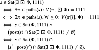
Boolean Connectives. The computation of the satisfaction sets for the Boolean connectives closely follows the semantic definition based on the da Costa algebra. Conjunction and disjunction are implemented using the usual intersection and union of sets, respectively. The set $\textrm{Sat}(\lnot \Phi ,b)$ is the complement of all states on which $\Phi$ evaluates to 1111 (recall that we assume $b > 0000$). Finally, the implementation of the implication is more involved. By definition, the set $\textrm{Sat}(\Phi \Rightarrow \Psi ,1111)$ is the set of states s for which $V(s,\Phi )$ is less than $V(s,\Psi )$; in set notation, this is expressed by the intersection of the sets $\textrm{Sat}(\Psi ,b) \cup (S{\setminus } \textrm{Sat}(\Phi ,b))$ for each $b\in \mathbb {B}_4$. For any other truth value $b \le 0111$, $\textrm{Sat}(\Phi \Rightarrow \Psi ,b)$ consists of all states where the implication evaluates to 1111 or $\Psi$ evaluates to at least b.

Temporal Operators. Now let us explain the characterization of the satisfaction sets for formulas with temporal operators. As the formulas can start with an existential or a universal operator, we discuss the satisfaction sets for them individually.

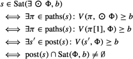
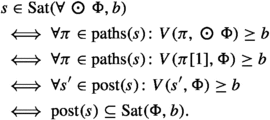
A state s satisfies the formula with a value of at least b if one of its successors satisfies $\Phi$ with a value of at least b. Hence, the set is the set of states s such that one of its successors is in $\textrm{Sat}(\Phi ,b)$. Dually, the set is the set of states s such that all of its successors are in $\textrm{Sat}(\Phi ,b)$.

As for CTL, we use fixed point equations over sets of states to compute satisfaction sets for rCTL formulas with the remaining temporal operators. So, let us first briefly describe some notation and useful properties of fixed point equations over sets of states. A function F that maps a set of states to another set of states is monotonic if $T_1\subseteq T_2$ implies $F(T_1) \subseteq F(T_2)$ for all sets $T_1, T_2$ of states. All monotonic functions have unique least and greatest fixed points [25]. Hence, given a monotonic function F (with variable T), we write $\textsf{lfp}\,T.F(T)$ and $\textsf{gfp}\,T.F(T)$ to denote the least fixed point and the greatest fixed point of F, respectively. All functions we consider in the following are monotonic.

We begin with formulas of the form . By definition, a state s satisfies with a value of at least b if there exists a path from s containing a state that satisfies $\Phi$ with a value of at least b. Since we are now dealing with paths, we can apply the expansion laws of rLTL [7]. In this particular case, we obtain the following statement: a state s satisfies with a value of at least b if and only if s satisfies $\Phi$ with a value of at least b or one of its immediate successors satisfies with a value of at least b. Hence, as in CTL, is the smallest subset T of S satisfying $\textrm{Sat}(\Phi ,b)\cup \{s\in S\mid \textrm{post}(s)\cap T\not = \emptyset \}\subseteq T$. That capture this via fixed point operators, we define the function

$$\begin{aligned} F^\exists (T,S_1,S_2) = S_1\cup \{s\in S_2 \mid \textrm{post}(s)\cap T\not = \emptyset \}. \end{aligned}$$

So, $F^\exists (T,S_1,S_2)$ contains all states in $S_1$ as well as all states in $S_2$ that have a successor in T. Note that this definition is more general than what we need it here, which will be useful for other temporal operators. But by fixing $S_1 = \textrm{Sat}(\Phi , b)$ and $S_2 = S$, we capture the expansion law of . Thus, consider the map

$$\begin{aligned} T \mapsto F^\exists (T, \textrm{Sat}(\Phi ,b), S) \end{aligned}$$

mapping sets of states to sets of states. We will prove that its fixed point $\textsf{lfp}\,T.F^\exists (T, \textrm{Sat}(\Phi ,b), S)$ is indeed the satisfaction set of .

Dually, a state s satisfies the formula with a value of at least b if every path starting from s contains a state satisfying $\Phi$ with value at least b. Using analogous arguments, one can show that the set is the least fixed point $\textsf{lfp}\,T. F^\forall (T,\textrm{Sat}(\Phi ,b),S)$, where $F^\forall$ is defined as

$$\begin{aligned} F^\forall (T,S_1,S_2) = S_1\cup \{s\in S_2 \mid \textrm{post}(s)\subseteq T\}. \end{aligned}$$

Next, we consider formulas of the form . The characterization of the set is more complex, and we discuss each truth value separately. Firstly, a state s satisfies with value 1111 if there exists a path from s on which every state satisfies $\Phi$ with value 1111. By again applying an expansion law similar to that of CTL, this statement is equivalent to s satisfying $\Phi$ with value 1111 and one of its successors satisfying with value 1111. Hence, the set equals the greatest fixed point $\textsf{gfp}\,T.F^\exists (T,\emptyset ,\textrm{Sat}(\Phi ,1111))$.

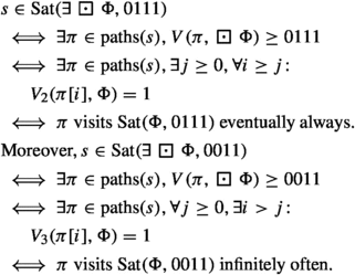
Next, a state s satisfies with a value of at least 0111 if there exists a path from s on which eventually every state satisfies $\Phi$ with a value of at least 0111. A set of states with such a property can be expressed using nested fixed points as usual (see Arnold and Niwinski [26] for details). We will prove that the set is equal to the nested fixed point

$$\begin{aligned} \textsf{lfp}\,T_1. \textsf{gfp}\,T_2. G^\exists (T_1,T_2,\emptyset ,\textrm{Sat}(\Phi ,0111)),\end{aligned}$$

where $G^\exists$ is defined as

$$\begin{aligned} G^\exists (T_1,T_2,S_1,S_2) = {}&S_1 \cup {} \\&\{s \in S \mid \textrm{post}(s)\cap T_1\not = \emptyset \} \cup {} \\&\{s\in S_2 \mid \textrm{post}(s)\cap T_2\not = \emptyset \}. \end{aligned}$$

Intuitively, the inner greatest fixed point in this nested fixed point represents the property of a path that all states on that path satisfy $\Phi$ with a value of at least 0111 (similar to the case of and truth value 1111 just discussed). Then, the outer least fixed point ensures that there exists a path that has a suffix with that property (similar to the case of discussed above).

Similarly, a state s satisfies with a value of at least 0011 if there exists a path from s on which there exist infinitely many states satisfying $\Phi$ with a value of at least 0011. Note that the property that a path contains infinitely many states satisfying $\Phi$ (with a value b) is the dual of the property that a path contains finitely many states satisfying $\Phi$ (with a value b). Hence, similar to the last case, it holds that

Finally, a state s satisfies with a value of at least 0001 if there exists a path from s containing a state that satisfies $\Phi$ with a value of at least 0001, which is equivalent to satisfying with a value of at least 0001. Hence, is the least fixed point $\textsf{lfp}\,T.F^\exists (T,\textrm{Sat}(\Phi ,0001),S)$, as in the case of .

Analogously, one can characterize using the fixed points of the functions $F^\forall$ and $G^\forall$, where

$$\begin{aligned} G^\forall (T_1,T_2,S_1,S_2) = {}&S_1 \cup {} \\&\{s \in S \mid \textrm{post}(s)\subseteq T_1\} \cup {} \\&\{s\in S_2 \mid \textrm{post}(s)\subseteq T_2\}. \end{aligned}$$

As the semantics of mimics the classical semantics, its characterization is generalized from that of , as for CTL. Hence, its characterization can be obtained using the functions $F^\exists$ and $F^\forall$. We describe the case , and the case  is again similar. A state s satisfies with a value of at least b if there exists a path from s containing a state that satisfies $\Psi$ with a value of at least b and every state before that in the path satisfies $\Phi$ with a value of at least b. By applying the expansion law of rLTL [7], this statement is equivalent to s satisfying $\Psi$ with a value of at least b or it satisfying $\Phi$ with a value of at least b and one of its successors satisfying with a value of at least b. Hence, as in CTL, is the smallest subset T of S satisfying $\textrm{Sat}(\Psi ,b)\cup \{s\in \textrm{Sat}(\Phi ,b)\mid \textrm{post}(s)\cap T\not = \emptyset \}\subseteq T$. This is captured by the map

$$\begin{aligned} T \mapsto F^\exists (T, \textrm{Sat}(\Psi ,b), \textrm{Sat}(\Phi ,b)). \end{aligned}$$

Therefore, the least fixed point

$$\begin{aligned} \textsf{lfp}\,T.F^\exists (T, \textrm{Sat}(\Psi ,b), \textrm{Sat}(\Phi ,b)) \end{aligned}$$

of the map is the satisfaction set of .

Finally, the semantics of is also defined using the counting interpretation described in Sect. 3, similarly to the semantics of . However, note that the satisfaction sets for are characterized only using the satisfaction sets for $\Phi$, whereas the satisfaction sets for must be characterized using the satisfaction sets of both formulas $\Phi$ and $\Psi$. Hence, the characterization for can be obtained using the similar fixed points as for but using the satisfaction sets of both formulas $\Phi$ and $\Psi$.

Example 2

Before proving that the characterization in Table 3 is correct, let us illustrate it on a simple Kripke structure, depicted in Fig. 1. Continuing the example presented in Sect. 1, the Kripke structure demonstrates the interaction between two agents, a robot and office workers (note that for simplicity we consider all workers as one agent). It captures which agent is present in the dock of the robot (for the sake of readability, we only consider one other location). Initially, only the robot is present in its dock, captured by the initial state $s_0$ of the Kripke structure. The robot can continue waiting in its dock, captured by the self-loop in $s_0$, or it can start performing its task, and, to do so, leave the dock. This is captured by the transition from state $s_0$ to $s_1$, where there are no agents present at the dock. Now, when no agents are present in the dock, represented by state $s_1$, the office workers can visit the dock, leading to state $s_2$. The robot can only return to the dock if it is vacant (encoded by state $s_1$), i.e., there is no edge from $s_2$ to $s_0$. Thus, office workers can prevent the robot from returning to its dock, but not continuously, as there is no self-loop in $s_2$: the office worker leaves the dock immediately.

For this Kripke structure, we now compute, for each state, the maximal truth values with which the state satisfies the subformulas of . If this value is b for some state s and some subformula $\Psi$, then we have $s \in \textrm{Sat}(\Psi , b')$ for all $b' \le b$ and $s \notin \textrm{Sat}(\Psi , b')$ for all $b' > b$.

These truth values are indicated below the corresponding state in Fig. 1.

Fig. 1

A Kripke structure that tracks a possible interaction between a robot and office workers. Within each state, we mention its identifier. Above each state, we mention its label. Below each state, we mention the maximal valuation that holds in the state for each subformula of

In Fig. 1, observe that R holds with a value of 1111 in the state $s_0$ and H holds with a value of 1111 in the state $s_2$ since $s_0$’s label contains R and $s_2$’s label contains H. This is consistent with our characterization of satisfiable set for atomic propositions, presented in Table 3: $\textrm{Sat}(R, 1111) =\{s_0\}$ and $\textrm{Sat}(H, 1111)=\{s_2\}$. Next, observe that the formula $\lnot H$ holds in states $s_0$ and $s_1$ with a value of 1111 since H does not hold in $s_0$ and $s_1$ with a value of 1111. This can be seen in the our characterization of negation: $\textrm{Sat}(\lnot H, 1111) = S{\setminus }\textrm{Sat}(H,1111) = S{\setminus }\{s_2\}=\{s_0,s_1\}$.

The formula holds in the states $s_0$ and $s_1$ with a value of 1111. This is because, both $\textrm{post}(s_0)$ and $\textrm{post}(s_1)$ contain a state in which R holds with a value of 1111, namely, the state $s_0$ for both cases. This is also reflected in our characterization of the next operator: . Also, holds in the state $s_2$ only with a value of 0000, as $\textrm{post}(s_2)$ does not contain a state where R holds with a value larger than 0000.

Observe that the formula  holds in all states with a value of 0011. This is because every path through the Kripke structure visits infinitely many states where $\lnot H$ holds, as $s_2$ does not have a self-loop. Hence, every state satisfies with at least 0011. This is exactly captured in our characterization for the always operator: (the computation of nested fixed points can be found in Arnold and Niwinski [26]). On the other hand, from every state there is a path that visits $s_2$ infinitely often, i.e., H holds infinitely often. Therefore, no state can satisfy with 0111. Again, this is captured in our characterization for the always operator: . Thus, holds in all states with a maximal value of 0011.

In a fashion similar to , the formula holds with a value of 0011 in all the states. This is also reflected in our characterization for the always operator.

Now, since the maximal value of is equal to that of in all the states, holds in all the states with a value of 1111. Also, our characterization of implication states .

Lemma 5

The characterization of the satisfaction sets in Table 3 is correct.

Proof

Let $M = (S,I,R,L)$ be a given Kripke structure and $b\in \mathbb {B}_4{\setminus }\{0000\}$. Now, we show that every equation in Table 3 using a case-by-case analysis.

• $\begin{aligned}&s\in \textrm{Sat}(p,b)\\&\iff V(s,p)\ge b>0000\\&\iff V(s,p) = 1111 \\&\iff p\in L(s). \end{aligned}$

• $\begin{aligned}&s\in \textrm{Sat}(\Phi \vee \Psi ,b)\\&\iff V(\Phi \vee \Psi )\ge b\\&\iff \max \{V(s,\Phi ),V(s,\Psi )\}\ge b\\&\iff V(s,\Phi )\ge b \text { or } V(s,\Psi )\ge b\\&\iff s\in \textrm{Sat}(\Phi ,b) \text { or } s\in \textrm{Sat}(\Psi ,b)\\&\iff s\in \textrm{Sat}(\Phi ,b) \cup \textrm{Sat}(\Psi ,b). \end{aligned}$

• $\begin{aligned}&s\in \textrm{Sat}(\Phi \wedge \Psi ,b)\\&\iff V(\Phi \wedge \Psi )\ge b\\&\iff \min \{V(s,\Phi ),V(s,\Psi )\}\ge b\\&\iff V(s,\Phi )\ge b \text { and } V(s,\Psi )\ge b\\&\iff s\in \textrm{Sat}(\Phi ,b) \text { and } s\in \textrm{Sat}(\Psi ,b)\\&\iff s\in \textrm{Sat}(\Phi ,b) \cap \textrm{Sat}(\Psi ,b). \end{aligned}$

• $\begin{aligned}&s\in \textrm{Sat}(\lnot \Phi ,b)\\&\iff V(s,\lnot \Phi ) \ge b \ge 0001\\&\iff \overline{V(s,\Phi )} = 1111\\&\iff V(s,\Phi ) \not = 1111\\&\iff s\in S{\setminus } \textrm{Sat}(\Phi ,1111). \end{aligned}$

• $\begin{aligned}&s\in \textrm{Sat}(\Phi \Rightarrow \Psi ,1111)\\&\iff \big (V(s,\Phi ) \rightarrow V(s,\Psi )\big ) = 1111\\&\iff V(s,\Phi ) \le V(s,\Psi ) \\&\iff \forall b\in \mathbb {B}_4 :s \not \in \textrm{Sat}(\Phi ,b){\setminus } \textrm{Sat}(\Psi ,b) \\&\iff \forall b\in \mathbb {B}_4 :s \in \big (S{\setminus } \textrm{Sat}(\Phi ,b)\big )\cup \textrm{Sat}(\Psi ,b)\\&\iff s \in \bigcap _b \textrm{Sat}(\Psi ,b) \cup (S{\setminus } \textrm{Sat}(\Phi ,b)). \end{aligned}$

  Similarly, for some $b\le 0111,$

  $\begin{aligned}&s\in \textrm{Sat}(\Phi \Rightarrow \Psi ,b)\\&\iff \big (V(s,\Phi ) \rightarrow V(s,\Psi )\big ) \ge b\\&\iff V(s,\Phi ) \le V(s,\Psi ) \text { or } V(s,\Psi ) = b\\&\iff s\in \textrm{Sat}(\Phi \Rightarrow \Psi ,1111) \cup \textrm{Sat}(\Psi ,b). \end{aligned}$

• 

  and

  

It remains to consider the temporal operators eventually, always, until, and release. Here, we need to prove that the fixed-point characterizations presented are correct. For most cases, the technical core of the arguments are standard characterizations of safety (a state formula holds at every state of a given path), co-Büchi (a state formula holds almost always on a given path), Büchi (a state formula holds infinitely often on a given path), and reachability (a state formula holds in at least one state of a given path) conditions. We present several cases in detail and refer for the other ones to the book by Arnold and Niwinski [26] for more details.

• 

  Hence, is a fixed point of the function $T \mapsto F^\exists (T,\textrm{Sat}(\Psi ,b),\textrm{Sat}(\Phi ,b))$. Now, we only need to show that it is indeed the least fixed point. Suppose $T'$is another fixed point of that function. If , then there exists a path $\pi = s_0s_1s_2\cdots$ and some $j>0$ such that $V(s_j,\Psi )\ge b$ and $V(s_i,\Phi ) \ge b$ for all $0\le i<j$. Then:

  • $s_j\in \textrm{Sat}(\Psi ,b) \subseteq T'$;

  • $s_{j-1}\in T'$, since $s_j\in \textrm{post}(s_{j-1}) \cap T'$ and $s_{j-1}\in \textrm{Sat}(\Phi ,b)$;

  • $s_{j-2}\in T'$, since $s_{j-1}\in \textrm{post}(s_{j-2}) \cap T'$ and $s_{j-2}\in \textrm{Sat}(\Phi ,b)$;

  • Applying this argument repeatedly yields $s_0\in T'$.

  So, . Therefore, is the least fixed point of $T \mapsto F^\exists (T,\textrm{Sat}(\Psi ,b),\textrm{Sat}(\Phi ,b))$. Similarly, it can be shown that is the least fixed point of $T \mapsto F^\forall (T,\textrm{Sat}(\Psi ,b),\textrm{Sat}(\Phi ,b))$.

• In the following, we use $\texttt{true}$ as syntactic sugar for some tautology, e.g., $p \vee \lnot p$. Then, is equivalent to and we have $\textrm{Sat}(\texttt{true},b) = S$.

  Hence,

  

  Similarly, we have

  

  as claimed.

• 

  Hence, is a fixed point of the function $T \mapsto F^\exists (T,\emptyset ,\textrm{Sat}(\Phi ,1111))$. Now, we only need to show that it is indeed the greatest fixed point. Now, suppose $T'$ is another fixed point. If $s_0\in T'$, then

  • since $s_0\in T'$, there exists a state $s_1\in \textrm{post}(s_0)\cap T'$;

  • since $s_1\in T'$, there exists a state $s_2\in \textrm{post}(s_0)\cap T'$;

  Applying this argument iteratively yields that there exists a path $s_0s_1\cdots$ starting from s such that $V(s_i,\Phi ) = 1111$ for each $i\ge 0$. Hence, , which implies . Therefore, is the greatest fixed point of $T \mapsto F^\exists (T,\emptyset ,\textrm{Sat}(\Phi ,1111))$.

  Similarly, the following holds

  

  A path visiting a set eventually always or infinitely often can be written in terms of nested fixed points as claimed (see Arnold and Niwinski [26] for details).

  

  Hence,

  

  as claimed.

  Analogously, one can show the claimed results for .

• For the operator , the claim can be shown using arguments similar to those for . $\square$

Algorithm 1 computes $5\cdot |\textrm{sub}(\Phi )|$ satisfaction sets following the subformula ordering. Using the standard fixed point iterations [27], the nested fixed points of depth two can be computed in time $\mathcal {O}(NK)$ on a Kripke structure with N vertices and K transitions [28]. So, we obtain the following.

Theorem 6

Given an rCTL formula $\Phi$ and a Kripke structure with N states and K transitions, the rCTL model checking problem can be solved in time $\mathcal {O}(NK|\Phi |)$.

Note that the CTL model checking algorithm also takes polynomial time in the size of the formula and the number of transitions of the Kripke structure [29]. Hence, both model checking problems are in $\textrm{PTIME}$. Moreover, a lower bound of the rCTL model checking problem can be derived from the $\textrm{PTIME}$ lower bound of CTL model checking [30] and Lemma 1. In total, we obtain the following result, showing that the CTL and rCTL model checking problems have the same asymptotic complexity.

Corollary 7

The model checking problem for rCTL is $\textrm{PTIME}$-complete.

3.5 rCTL and the modal $\mu$-calculus

In the previous section, we have seen that one can solve the rCTL model checking problem by computing least and greatest fixed points. In this section, we show that every rCTL formula can be translated into an equivalent formula of the modal $\mu$-calculus [31], i.e., modal logic with least and greatest fixed points. This is not necessarily surprising, as most temporal logics can be translated into the modal $\mu$-calculus [32]. However, the result is very useful to settle the complexity of satisfiability and synthesis, which we achieve by reductions to satisfiability and synthesis for the modal $\mu$-calculus.

We begin by reviewing the basic definitions of the modal $\mu$-calculus. It consists of state formulas only, which are constructed from atomic propositions with Boolean connectives, the temporal operators and , as well as the least ($\mu$) and the greatest ($\nu$) fixed point operator.

Formally, given a set $\mathcal {P}$ of atomic propositions and a set $\mathcal{P}\mathcal{V}$ of atomic proposition variables, $\mu$-calculus formulas are given by the grammar

where $p\in \mathcal {P}$ and $y \in \mathcal{P}\mathcal{V}$. As usual, we require that in subformulas of the form $\mu y. \Phi$ and $\nu y.\Phi$, every free occurrence of y in $\Phi$ is under the scope of an even number of negations. For further details, we refer the reader to standard literature on this topic, e.g., Grädel, Thomas, and Wilke [33].

Unlike temporal logics, the semantics of the $\mu$-calculus is naturally defined using satisfaction sets. Given a Kripke structure $M=(S,I,R,L)$, the satisfaction sets are defined with respect to a variable function $v:\mathcal{P}\mathcal{V}\rightarrow 2^S$ that maps each atomic proposition variable to a set of states. Moreover, for a subset $T\subseteq S$, let $v[y\rightarrow T]$ denote the variable function that maps y to T while preserving the value of $v$ for every other input.

Given a variable function $v$ and a $\mu$-calculus formula $\Phi$, let $\textrm{Sat}_{\mu }^v(\Phi )$ denote the set of states satisfying $\Phi$ with respect to $v$. These sets are defined recursively using the least and greatest fixed points, as shown in Table 4. The functions the fixed point operators are applied to are monotonic since every occurrence of a fixed point variable is under an even number of negations. Hence, the fixed points all exist.

For $\mu$-calculus sentences, i.e., formulas without free variables, the satisfaction sets $\textrm{Sat}_\mu ^v$ are independent of $v$. Hence, we drop the parameter $v$ from the notation whenever possible.

Table 4 Characterization of the satisfaction sets for $\mu$-calculus formulas

We now show that, like other temporal logics, rCTL can also be translated into the modal $\mu$-calculus. As before, we say an rCTL formula $\Phi$ with a truth value $b\in \mathbb {B}_4$ is equivalent to a $\mu$-calculus sentence $\Phi '$ if for every Kripke structure it holds that $\textrm{Sat}(\Phi ,b) = \textrm{Sat}_\mu (\Phi ')$. Then we have the following result.

Theorem 8

For every rCTL formula and truth value, there is an equivalent $\mu$-calculus sentence of linear size.

Proof

We show that there exists a mapping t that assigns to every rCTL formula $\Phi$ and truth value $b\in \mathbb {B}_4$ an equivalent $\mu$-calculus formula $t(\Phi ,b)$. We define this mapping recursively, starting with the atomic rCTL formulas. In the following proof, we use $\texttt{true}$ as syntactic sugar for an arbitrary tautology of the $\mu$-calculus, e.g., $p \vee \lnot p$.

First of all, for any rCTL formula $\Phi$ with truth value 0000, a trivial equivalent $\mu$-calculus formula is $t(\Phi ,0000) = \texttt{true}$. Furthermore, comparing the characterization of the satisfaction sets of rCTL and the $\mu$-calculus (Tables 3 and 4), one can see that for a Boolean combination of rCTL formulas $\Phi$ and $\Psi$ with any truth value $b\in \mathbb {B}_4\setminus \{0000\}$, the following recursive translations indeed results in an equivalent $\mu$-calculus formula:

$$\begin{aligned} t(p, b)&= p \text { for each }p\in \mathcal {P},\\ t(\Phi \vee \Psi , b)&= t(\Phi , b) \vee t(\Psi , b), \\ t(\Phi \wedge \Psi , b)&= t(\Phi , b) \wedge t(\Psi , b), \\ t(\lnot \Phi , b)&= \lnot t(\Phi ,1111). \end{aligned}$$

Moreover, we have

$$\begin{aligned} t(\Phi \Rightarrow \Psi ,1111)&= \bigwedge _{b} t(\Psi ,b)\vee \lnot t(\Phi ,b), \end{aligned}$$

and

$$\begin{aligned} t(\Phi \Rightarrow \Psi ,b)&= t(\Phi \Rightarrow \Psi ,1111) \vee t(\Psi ,b) \end{aligned}$$

for any $b\le 0111$.

The rCTL formulas with the next operator are captured by applying the $\mu$-calculus operators and as follows for $b\in \mathbb {B}_4\setminus \{0000\}$:

For rCTL formulas with other temporal operators, the satisfaction sets (in Table 3) are defined using fixed points of functions $F^\exists$, $F^\forall$, $G^\exists$, and $G^\forall$. Hence, we first give $\mu$-calculus formulas that capture these functions. Note that if the sets $T,S_1,S_2$ are the satisfaction sets of the rCTL formulas $\Phi _t,\Phi _1,\Phi _2$ with truth values $b_t,b_1,b_2$, respectively, then it holds that

Now, suppose that the $\mu$-calculus formula $t(\Phi _1,b_1)$ is equivalent to the rCTL formula $\Phi _1$ with truth value $b_1$, and the $\mu$-calculus formula $t(\Phi _2,b_2)$ is equivalent to the rCTL formula $\Phi _2$ with truth value $b_2$. Then, we have

Therefore, for $\mu$-calculus formulas $\Phi _1'$ and $\Phi _2'$, the function $F^\exists$ can be represented by the following $\mu$-calculus formula containing y as a free variable:

Hence, using Table 3, one can see that an equivalent $\mu$-calculus formula for the rCTL formula with truth value $b\in \mathbb {B}_4{\setminus } \{0000\}$ is the following:

Similarly, the functions $F^\forall$, $G^\exists$, and $G^\forall$ can be represented by the following $\mu$-calculus formulas:

Now, for an rCTL formula with temporal operators , , , and , we obtain an equivalent $\mu$-calculus formula of linear size from the characterization of satisfaction sets given in Table 3 by replacing the functions and the satisfaction sets of subformulas with corresponding $\mu$-calculus formulas. $\square$

While it is true that every CTL formula can be transformed into an equivalent alternation-free (with alternation depth 1, as defined in [34]) $\mu$-calculus formula, it is important to note that the constructed $\mu$-calculus formulas for rCTL formulas typically have an alternation depth of at most 2. This limitation arises from the presence of two-depth alternation for some rCTL operators, such as with value 0011 as illustrated in Table 3. Furthermore, as the model checking problem for $\mu$-calculus formulas with alternation depth d can be solved in time $\mathcal {O}(n^{d+1})$ [34, 35], one can also solve rCTL model checking in cubic time by reducing it to $\mu$-calculus model checking.

Let us conclude by mentioning that the converse of Theorem 8 does not hold: rCTL is strictly less expressive than the modal $\mu$-calculus. This follows from a stronger result presented to be presented in Sect. 5.3.

3.6 rCTL satisfiability

This section considers the satisfiability problem for rCTL, which is: given an rCTL formula $\Phi$ and a truth value $b_0\in \mathbb {B}_4$, does there exist a Kripke structure $M = (S,I,R,L)$ such that $I\subseteq \textrm{Sat}(\Phi ,b_0)$? The next theorem settles the complexity of the rCTL satisfiability problem.

Theorem 9

The satisfiability problem for rCTL is $\textrm{EXPTIME}$-complete.

Proof

The upper bound is obtained by translating a given rCTL formula and a given truth value into an equivalent $\mu$-calculus formula of linear size (see Theorem 8) and then checking the resulting formula for satisfiability. Since the satisfiability problem for the $\mu$-calculus (defined as expected) is $\textrm{EXPTIME}$-complete [36], rCTL satisfiability is in $\textrm{EXPTIME}$ as well.

The matching lower bound already holds for CTL satisfiability (again defined as expected) [37], which, due to Lemma 1, reduces to rCTL satisfiability. $\square$

Moreover, since every satisfiable formula of the $\mu$-calculus has a model of exponential size [38], the same is true for rCTL.

Corollary 10

Every satisfiable rCTL-formula has a model of exponential size.

There are satisfiable CTL formulas that have only models of at least exponential size [39].² Thus, the upper bound in Corollary 10 is tight.

Also, note that the asymptotic complexity of the rCTL satisfiability problem and the size of a model matches that of CTL.

3.7 rCTL synthesis

We now turn to the problem of rCTL synthesis. The synthesis problem asks, given an rCTL specification on the input–output behavior of a system, whether there is a system satisfying the specification, and, if yes, compute one. As a preparatory step, let us first introduce the required notation.

Let $\mathcal {P} = \mathcal {I} \cup \mathcal {O}$ be the disjoint union of a set $\mathcal I$ of input propositions and a set $\mathcal O$ of output propositions. A strategy is a mapping $f:(2^\mathcal {I})^* \rightarrow 2^\mathcal {O}$. Note that finite automata with input alphabet $2^{\mathcal {I}}$ and output alphabet $2^{\mathcal {O}}$ (with Mealy or Moore semantics) can be used to implement strategies. We call such strategies finite-state and measure their size in the number of states of the automaton.

A strategy $f$ induces an infinite Kripke structure $M_f= (S, I, R, L)$ with $S = (2^\mathcal {I})^+$, $I = 2^\mathcal {I}$, $R = \{(w, wa) \mid w \in (2^\mathcal {I})^+, a \in 2^\mathcal {I}\}$, and $L(wa) = a \cup f(wa)$.

We say that $f$ realizes an rCTL formula $\Phi$ with at least value $b_0 \in \mathbb {B}_4$ if $V(s,\Phi ) \ge b_0$ for all initial states s of $M_f$. Further, a rCTL formula is realizable with at least value $b_0$ if there is a strategy that realizes it with at least $b_0$. The rCTL synthesis problem is: given an rCTL formula $\Phi$ and a truth value $b_0 \in \mathbb {B}_4$, is $\Phi$ realizable with at least $b_0$? The next theorem settles its complexity.

Theorem 11

The rCTL synthesis problem is $\textrm{EXPTIME}$-complete.

Proof

The upper bound is obtained by translating a given rCTL formula and a given truth value into an equivalent $\mu$-calculus formula of linear size (see Theorem 8) and then checking the resulting formula for realizability (which is defined as expected). Since the synthesis problem for the $\mu$-calculus is $\textrm{EXPTIME}$-complete [40], rCTL synthesis is in $\textrm{EXPTIME}$ as well.

The matching lower bound already holds for CTL synthesis [41], which, due to Lemma 1, reduces to rCTL synthesis. $\square$

As every realizable formula of the $\mu$-calculus is realized by a finite-state strategy of exponential size, which can be computed in exponential time [41], the same is true for rCTL.

Corollary 12

If an rCTL-formula $\varphi$ is realizable with at least $b_0$, then one can compute, in exponential time, an exponentially-sized finite-state strategy realizing $\varphi$ with at least $b_0$.

There are realizable CTL formulas that are only realized by finite-state strategies of exponential size: this follows from the exponential lower bound on the size of model (see the discussion below Corollary 10) and the fact that satisfiability can be reduced to synthesis [41]. Hence, the upper bound in Corollary 12 is tight.

Finally, note that Theorem 11 and Corollary 12 imply that the rCTL synthesis problem again has the same asymptotic complexity as the one for CTL.

4 Review of CTL*

In this section, we briefly review the syntax and semantics of CTL*, which we then robustify to obtain robust CTL*.

4.1 Syntax

Unlike CTL, CTL* allows path quantifiers $\exists$ and $\forall$ to be arbitrarily nested with temporal operators. The syntax of CTL* state formulas is the same as in CTL. Moreover, CTL* path formulas are similar to LTL formulas. Consequently, CTL* state formulas over $\mathcal {P}$ are formed according to the grammar

$$\begin{aligned} \Phi {:}{:}=p \mid \Phi \vee \Phi \mid \Phi \wedge \Phi \mid \lnot \Phi \mid \Phi \Rightarrow \Phi \mid \exists \varphi \mid \forall \varphi , \end{aligned}$$

where $p\in \mathcal {P}$ and $\varphi$ is a path formula. CTL* path formulas are formed according to the grammar

4.2 Semantics

Let M be a Kripke structure, $\Phi$, $\Psi$ two CTL* state formulas, and $\varphi$, $\psi$ two CTL* path formulas. For a state s, the CTL* semantics $V_{\text {{CTL*}}}(s,\Phi )$ is defined as the CTL semantics (see Sect. 2.2). For a path $\pi$, the semantics is analogous to the LTL semantics via a valuation function $V_{\text {{CTL*}}}$:

5 Robust CTL*

In this section, we present the robust version of CTL*, named robust CTL*, which combines the features of rCTL and rLTL. We show that rCTL* is more expressive than both. In addition, we present an rCTL* model checking algorithm and address the rCTL* satisfiability and synthesis problems.

5.1 Syntax

Like CTL*, robust CTL* allows path quantifiers $\exists$ and $\forall$ to be arbitrarily nested with temporal operators. The syntax of rCTL* state formulas is the same as in rCTL and CTL*. Moreover, rCTL* path formulas are similar to rLTL formulas, with the only difference being the use of arbitrary rCTL* state formulas as atoms. Consequently, rCTL* state formulas over $\mathcal {P}$ are formed according to the grammar

$$\begin{aligned} \Phi {:}{:}=p \mid \Phi \vee \Phi \mid \Phi \wedge \Phi \mid \lnot \Phi \mid \Phi \Rightarrow \Phi \mid \exists \varphi \mid \forall \varphi , \end{aligned}$$

where $p\in \mathcal {P}$ and $\varphi$ is a path formula. rCTL* path formulas are formed according to the grammar

Again, the set of subformulas of a state formula $\Phi$ is denoted by $\textrm{Sub}(\Phi )$ and the size of a formula is defined as the number of its syntactically different subformulas.

5.2 Semantics

As in CTL*, the semantics for rCTL* state and path formulas are analogous to the rCTL and rLTL semantics, respectively. In what follows, let M be a Kripke structure, $\Phi$, $\Psi$ two rCTL* state formulas, and $\varphi$, $\psi$ two rCTL* path formulas.

For a state s, the rCTL* semantics $V(s,\Phi )$ is then the same as the rCTL semantics (see Sect. 3.2).

For a path $\pi$, the semantics is analogous to the rLTL semantics (cf. Tabuada and Neider [7]) via a valuation function V (note that, for notational convenience, we use the letter V both the rCTL and the rCTL* valuation function):

Before studying the properties of rCTL*, let us illustrate the difference between rCTL and rCTL* using an example.

Example 3

Continuing our running example from Sect. 1, we illustrate how the rCTL* formula is different from the rCTL formula from Examples 1 and 2. Recall that $\lnot H$ states that office workers are not at the robot’s dock and states that the robot can return to its dock in one time step. Assume evaluates to 1111. Then the formula must evaluate to 1111 for each path. Hence, the following holds:

• If $\lnot H$ holds at every state in a path $\pi$, then evaluates to 1111. Hence, by the rCTL* semantics, must also evaluate to 1111. That means, also holds at every state in $\pi$. Hence, in any path, if office workers never visit the dock, then from every state, the robot can return to its dock in one time step.

• Similarly, if $\lnot H$ holds eventually always for some path $\pi$, then evaluates to 0111. Then, by the rCTL* semantics, evaluates to 0111 or higher. Hence, also needs to hold eventually always in $\pi$. Therefore, if office workers visit the dock a few times and never visit it again in a path, then from any state in that path, the robot can return to its dock eventually.

• Similarly, if $\lnot H$ holds at infinitely (finitely) many states in some path $\pi$, then needs to hold at infinitely (finitely) many states in $\pi$.

As we can see, the rCTL* formula  captures the robustness property for every path separately, whereas the rCTL formula  captures the robustness property jointly for all paths starting from a state.

Fig. 2

The Kripke structure for Example 3. States are labeled with the formulas that hold at that state with truth value 1111

To understand the difference, let us consider the Kripke structure M with initial state $s_0$ as shown in Fig. 2 (where transitions are depicted by edges). Suppose the set of states that satisfy (with value 1111) the state formulas $\lnot H$ and are $\{s_0,s_1\}$ and $\{s_0,s_2\}$, respectively (as shown by the labels in the figure).

There are only two paths starting from $s_0$, i.e., $\pi _1 = s_0 s_1 s_1 \cdots$ and $\pi _2 = s_0 s_2 s_2 \cdots$. Since $\lnot H$ holds at every state in the path $\pi _1$, we have . Moreover, since $\lnot H$ holds only at the first state in the path $\pi _2$, we have . Hence, . Similarly, since holds only at the first state of each path, we have . Hence, . Therefore, it holds that according to the rCTL semantics.

Now, let us consider the rCTL* formula . As we have , it holds that . Similarly, we have . Hence, we have according to the rCTL* semantics.

Recall that the rCTL formula  evaluates at state s to $1111 \ne 0001$. This is the case because both of the paths do not satisfy with value 1111 individually, but collectively, the state $s_0$ satisfies .

5.3 Expressiveness of rCTL*

The satisfaction sets and the equivalence between two formulas in rCTL* are defined as for rCTL. As we can see, rCTL* is an extension of both rCTL and rLTL. Therefore, it subsumes both rCTL and rLTL (and hence, it also subsumes CTL and LTL). Furthermore, by Corollary 4, there exist rCTL formulas that are not expressible in rLTL and vice versa. In total, we obtain the following result.

Theorem 13

rCTL* is more expressive than rLTL, rCTL, CTL, and LTL.

Using the same idea as in Lemma 1, one can recover the CTL* semantics of a formula with no implication from the first component of the rCTL* semantics. Conversely, using the same arguments as for the analogous result for rLTL [7, Proposition 5], one can translate each rCTL* formula into four CTL* formulas that captures the four components of the rCTL* semantics. Hence, we obtain the following result.

Theorem 14

CTL* and rCTL* are equally expressive.

Proof

For any CTL* formula $\Phi$ containing no implication, let $\Phi _r$ be the rCTL* formula obtained by dotting all temporal operators in $\Phi$. Then for any state s, it holds that $V_{\text {CTL}}(s,\Phi ) = V_1(s,\Phi _r)$, which is shown as the analogous result for CTL and rCTL (see the proof of Lemma 1). Consequently, it holds that $\textrm{Sat}_{\text {CTL*}}(\Phi ) = \textrm{Sat}(\Phi _r,1111).$ Furthermore, as $\Phi \Rightarrow \Psi$ is equivalent to $\Psi \vee \lnot \Phi$ in CTL*, every CTL* formula can be rewritten as a formula containing no implication. Therefore, for every CTL* formula, there is an equivalent rCTL* formula with respect to the truth value 1111.

For the other direction, we define a mapping t that assigns to every rCTL* state formula $\Phi$ and truth value b an equivalent CTL* formula $t(\Phi ,b)$. Furthermore, t maps every rCTL* path formula $\varphi$ and a truth value b to $t(\varphi , b)$ such that for every path $\pi$,

$$\begin{aligned} V_{CTL^*}(\pi ,t(\varphi ,b)) = 1 \text { if and only if } V(\pi ,\varphi ) \ge b. \end{aligned}$$

Again, for $b=0000$, we can define $t(\Phi , b) = \texttt{true}$ for every state formula $\Phi$, where $\texttt{true}$ is an arbitrary tautology of CTL*, e.g., $p \vee \lnot p$.

In the following, we assume $b > 0000$. Then, for state formulas $\Phi$ and $\Psi$, the mapping t is defined inductively as follows:

$$\begin{aligned} t(p, b)&= p \text { for any }p\in \mathcal {P}, \\ t(\Phi \vee \Psi , b)&= t(\Phi , b) \vee t(\Psi , b), \\ t(\Phi \wedge \Psi , b)&= t(\Phi , b) \wedge t(\Psi , b), \\ t(\lnot \Phi , b)&= \lnot t(\Phi ,1111). \end{aligned}$$

Moreover, we define

$$\begin{aligned} t(\Phi \Rightarrow \Psi ,1111)&= \bigwedge _{b > 0000} t(\Psi ,b)\vee \lnot t(\Phi ,b), \end{aligned}$$

and

$$\begin{aligned} t(\Phi \Rightarrow \Psi ,b)&= t(\Phi \Rightarrow \Psi ,1111) \vee t(\Psi ,b) \end{aligned}$$

for each $b\le 0111$.

For Boolean combinations of path formulas, the mapping t can be defined analogously as for state formulas. For path formulas $\varphi$ and $\psi$ with temporal operators, t is defined as follows:

A structural induction shows that the translation t has the desired property. $\square$

Although we do not require the result, let us just mention that Theorem 14 also gives a translation of rCTL* into the modal $\mu$-calculus: rCTL* can be translated into CTL*, which can be translated into the modal $\mu$-calculus [32]. Conversely, the modal $\mu$-calculus is strictly more expressive than CTL* (see, e.g., Demri, Goranko, and Lange [42, Chapter 10]). Hence, it is also strictly more expressive than rCTL* (due to Theorem 14) and rCTL (which is a fragment of rCTL*).

5.4 rCTL* model checking

The model checking problem for rCTL* is analogous to that of rCTL: for a given finite Kripke structure $M = (S,I,R,L)$, an rCTL* formula $\Phi$ and a truth value $b_0\in \mathbb {B}_4$, does $V(s,\Phi ) \ge b_0$ hold for all initial states $s\in I$? One way of solving the rCTL* model checking problem is by applying the translation from rCTL* into CTL* (see Theorem 14) and then apply a CTL* model checking algorithm.

Here, we will present an alternative approach via a combination of rCTL and rLTL model checking. This approach is analogous to the classical CTL* model checking algorithm, is a combination of CTL and LTL model checking. In practice, the choice for one algorithm over the other depends on whether one wants to apply an CTL* model checker or an rLTL model checker.

As in rCTL, for the rCTL* model checking, we use the characterization of the satisfaction sets. $\textrm{Sat}(\Phi ,b)$ can be computed using Table 3 for every state formula $\Phi$ which is either an atomic proposition or can be expressed as a Boolean combination (conjunction, negation, etc.) of two subformulas. Otherwise, we use an rLTL model checking algorithm to compute $\textrm{Sat}(\Phi ,b)$ for a state formula starting with a path quantifier.

Let us first go through the basic concepts of rLTL and its model checking algorithm. As we have described earlier, rCTL* is an extension of rLTL. Both rCTL* path formulas and rLTL formulas are defined using almost the same syntax, with the only difference being the use of state formulas as atoms in rCTL*. Moreover, the valuation V for rLTL formulas is defined the same way as it is defined for rCTL* path formulas. The rLTL model checking problem is: given a Kripke structure M, an rLTL formula $\varphi$, and a truth value $b_0\in \mathbb {B}_4$, determine whether for all initial states s and all $\pi \in \textrm{paths}(s)$, it holds that $V(\pi ,\varphi )\ge b_0$.³ To solve the rLTL model checking problem, Tabuada and Neider [7] have provided an algorithm to compute a generalized Büchi automaton (see Grädel, Thomas and Wilke [33] for a definition) recognizing all traces over the alphabet $2^{\mathcal {P}}$ satisfying a given formula with a value $b\in B$ for a given set $B\subseteq \mathbb {B}_4$, as formalized below.

Lemma 15

(Tabuada and Neider [7]) Given an rLTL formula $\varphi$, and a set of truth values $B\subseteq \mathbb {B}_4$, one can construct a generalized Büchi automaton $A_{\varphi ,B}$ with $\mathcal {O}(5^{|\varphi |})$ states and $\mathcal {O}(|\varphi |)$ accepting sets that recognizes all paths $\pi$ such that $V(\pi ,\varphi ) \in B$.

One can now solve the rLTL model checking problem by first translating M into a Büchi automaton $A_M$ accepting exactly the traces labeling the paths of M starting in an initial state. Then, one determines whether $L(A_M)\cap L(A_{\varphi ,\{ b \in \mathbb {B}_4 \mid b < b_0 \}})$ is empty.

Coming back to computing $\textrm{Sat}(\Phi ,b)$ for $\Phi$ starting with a path quantifier, let us consider $\Phi = \forall \varphi$. Observe that $s\in \textrm{Sat}(\forall \varphi ,b)$ if and only if $V(s,\forall \varphi )\ge b$. Further, $V(s,\forall \varphi )\ge b$ if and only if $V(\pi ,\varphi )\ge b \text { for all }\pi \in \textrm{paths}(s)$. The basic idea is now to replace all maximal proper state subformulas $\Psi$ of $\varphi$ by fresh atomic propositions $a_{\Psi }$ and use the rLTL model checking algorithm to compute all the states from which all paths satisfy the rLTL formula $\varphi$ with value at least b. However, we need to make a minor modification in the construction of the Büchi automaton of Lemma 15 such that for each $a_{\Psi }$, it holds that $V(s,a_{\Psi }) \ge b$ whenever $s\in \textrm{Sat}(\Psi ,b)$ and $V(s,a_{\Psi }) < b$ whenever $s\not \in \textrm{Sat}(\Psi ,b)$. This can be done by initializing these atomic propositions with the required truth value.

Similarly, we compute $\textrm{Sat}(\exists \varphi ,b)$ by the rLTL model checking algorithm using the observation that $s\not \in \textrm{Sat}(\exists \varphi ,b)$ if and only if $V(\pi ,\varphi )< b \text { for all }\pi \in \textrm{paths}(s)$.

Now, one can solve the rCTL* model checking problem using Algorithm 1. However, the time complexity of the algorithm is not the same as in rCTL since the computation of $\textrm{Sat}$ uses the rLTL model checking algorithm, which takes exponential time in the size of the formula and the Kripke structure (Tabuada and Neider [7]). Hence, the time complexity of the rCTL* model checking algorithm is dominated by the time complexity of the rLTL model checking algorithm.

Altogether, our algorithm runs in polynomial space (as rLTL model checking is in $\textrm{PSPACE}$ [7]). A matching lower bound already holds for CTL* [43].

Theorem 16

The rCTL* model checking problem is $\textrm{PSPACE}$-complete.

The CTL* model checking problem is also $\textrm{PSPACE}$-complete [43]. Hence, both the CTL* and the rCTL* model checking problem have the same asymptotic complexity.

5.5 rCTL* satisfiability

This section considers the satisfiability problem for rCTL*, which is: for a given rCTL* formula $\Phi$ and truth value $b_0\in \mathbb {B}_4$, does there exist a Kripke structure $M = (S,I,R,L)$ such that $I\subseteq \textrm{Sat}(\Phi ,b_0)$?

Theorem 17

The satisfiability problem for rCTL* is $\textrm{2EXPTIME}$-complete.

Proof

Both the upper and the lower bound follow immediately from Theorem 14 and the fact that CTL* satisfiability (which is defined as expected) is $\textrm{2EXPTIME}$-complete [36]. The linear translation from rCTL* to CTL* yields the upper bound while the linear translation from CTL* to rCTL* yields the lower bound. $\square$

Furthermore, as every satisfiable CTL* formula has a model of doubly-exponential size (see, e.g., Demri, Goranko, and Lange [42, Chapter 15]), the same is true for rCTL*.

Corollary 18

Every satisfiable rCTL* formula has a model of doubly-exponential size.

There are satisfiable CTL* formulas that have only models of doubly-exponential size (see, e.g., Demri, Goranko, and Lange [42, Chapter 15]). Hence, the upper bound in Corollary 18 is tight.

Also, note again that the asymptotic complexity of the rCTL* satisfiability problem and the size of a model matches that of CTL*.

5.6 rCTL* synthesis

The notions of a strategy realizing an rCTL formula with at last value $b_0$ and an rCTL formula being realizable can be generalized to rCTL*. Then, the rCTL* synthesis problem is defined analogously to the rCTL synthesis problem: given an rCTL* formula $\Phi$ and a truth value $b_0 \in \mathbb {B}_4$, is $\Phi$ realizable with value at last $b_0$?

Theorem 19

The rCTL* synthesis problem is $\textrm{2EXPTIME}$-complete.

Proof

The lower bound again follows immediately from CTL* synthesis (again defined as expected) being $\textrm{2EXPTIME}$-complete [41] and the fact that the CTL* semantics is a special case of rCTL* (see Theorem 14).

Here, the upper bound follows from the converse translation, i.e., given a rCTL* formula $\Phi$ and a truth value $b_0 \in \mathbb {B}_4$, Theorem 14 allows us to construct (in linear time) a CTL* formula $t(\Phi ,{b_0})$ that is equivalent to $\Phi$ with respect to $b_0$: a strategy realizes $\Phi$ with at least $b_0$ if and only if it realizes $t(\Phi ,{b_0})$. As CTL* synthesis is in $\textrm{2EXPTIME}$ [41], we obtain the desired upper bound. $\square$

As every realizable CTL* formula is realized by a finite-state strategy of doubly-exponential size [41], which can be computed in doubly-exponential time, the same is true for rCTL*.

Corollary 20

If an rCTL*-formula $\Phi$ is realizable with at least $b_0$, then one can compute, in doubly-exponential time, a doubly-exponentially-sized finite-state strategy realizing $\varphi$ with at least $b_0$.

There are realizable LTL formulas (and therefore CTL* formulas, as LTL is a fragment of CTL*) that are only realized by finite-state strategies with at least doubly-exponentially many states [44]. Hence, the doubly-exponential upper bound in Corollary 20 is tight.

Perhaps unsurprisingly at this point, the asymptotic complexity of the rCTL* synthesis problem and the tight bound on the size of a finite-state strategy realizing an rCTL* specification match those of CTL*.

6 Related works

Numerous efforts have been made to formalize the concept of robustness in cyber-physical systems within the framework of formal methods. This section offers an extensive yet not exhaustive overview of various formalizations of robustness. We initiate our discussion with a series of approaches that necessitate designers to provide additional information alongside their desired specifications.

In the work by Bloem et al. [1], two quantitative robustness concepts are combined into a unified framework for robust synthesis. The first concept, known as robustness for safety, examines how frequently assumptions and guarantees are violated, with a requirement that their ratio remains bounded by a parameter $k\in \mathbb {N}$ (referred to as k-robustness). This counting process relies on error functions supplied by the designer. The second concept, robustness for liveness, deals with specifications in the form of

where $p_i$ and $q_j$ are atomic propositions. It compares the number of violated assumptions to the number of violated guarantees. While our semantics can distinguish between different ways of specification violations, it does not distinguish between the violation of one assumption and multiple assumptions. Consequently, this second approach is not directly comparable to the one proposed here. Furthermore, we do not make a distinction between safety and liveness properties.

In another work by Bloem et al. [45], a distinct framework for robust synthesis is introduced, which does not encompass the previously mentioned framework. This framework considers various notions of robustness, such as a system being robust if it satisfies a guarantee even when a finite number or even all of its inputs are hidden or misread, or when the assumptions are violated either finitely or infinitely often. Many of these notions align with our notion, and our definition of robustness allows systems to satisfy weaker guarantees whenever the assumptions are also weakened, making it more general. However, we cannot directly compare our approach with the notions of robustness in [45] that involve counting the number of violations since our semantics distinguishes only between zero, finite, and infinite violations of a specification.

In the work of Rodionova et al. [46], a connection is established between MTL/LTL and Linear Time-Invariant (LTI) filtering. Specifically, it is demonstrated that LTI filtering corresponds to MTL if addition and multiplication are interpreted as max and min operations, and if true and false are interpreted as one and zero, respectively. Different filtering kernels are employed to express weaker or stronger interpretations of the same formula, placing the burden on the designer to choose kernels and use multiple semantics to reason about how weakening assumptions affect guarantees.

In contrast to the approaches mentioned above, which necessitate designers to provide robustness metrics, our approach simplifies the designer’s task by requiring only the desired specification without the need for additional metrics. This simplification is especially beneficial as it may not always be clear which quantitative metric leads to the desired qualitative behavior.

In the realm of software systems, Zhang et al. [47] define robustness as the largest set of deviating environmental behaviors under which the system still guarantees a desired property. Therefore, robustness is defined as the set of all deviations under which a system continues to satisfy that property. While this work focuses on computing robustness rather than characterizing it, it is possible that certain temporal deviations could be expressed in our semantics. Additional noteworthy works, although not directly comparable to the methods described here, include Chaudhuri et al. [48] and Majumdar et al. [49], which consider continuity properties of software expressed by the requirement that a deviation in a program’s input causes a proportional deviation in its output. However, these notions of robustness only apply to the Turing model of computation and not to the reactive model of computation employed in this paper.

Several works have explored the robustness of specifications when reasoning over real-valued, continuous-time signals, with prominent examples being Fainekos et al. [50], Donze et al. [51], Akazaki et al. [52], Abbas et al. [53], and Mehdipour et al. [54]. In these works, specific choices made when crafting many-valued semantics are not discussed in detail. Notably, the notion of “time robustness” in [51] is somewhat similar to that of our semantics in that it measures the time needed for the truth value of a formula to change. However, in this line of work, robustness is derived from the real-valued nature of signals, whereas our semantics reasons over the more classical setting of discrete-time and Boolean-valued signals, with robustness derived from the temporal evolution of these signals. Consequently, these works on real-valued signals [50,51,52,53,54] and their extensions can be considered orthogonal and complementary to our approach.

Another relevant approach involving multi-valued extensions of LTL is presented in Almagor et al. [55]. This work introduces two quantitative extensions of LTL, one with propositional quality operators denoted as LTL$[\mathcal {F}]$, parameterized by a set $\mathcal {F}$ of functions over [0, 1], and another with discounting operators termed LTL$^{disc}[\mathcal {D}]$, parameterized by a set $\mathcal {D}$ of discounting functions. Both logics employ a many-valued variant of LTL to reason about quality, and the satisfaction value of a specification is a number in the interval [0, 1], which describes the quality of satisfaction. While the use of many-valued semantics in the context of quality aligns with that of robustness, there are notable differences. In particular, our notion of robustness or quality is intrinsic to the logic, while the approach in [55] requires designers to provide their own interpretation through sets $\mathcal {F}$ or $\mathcal {D}$ of functions. Moreover, there are several choices for defining logical connectives on the interval [0, 1], and the suitability of Gödel’s conjunction used in [55] for formalizing quality is not explicitly addressed. In contrast, we meticulously discuss and motivate all the choices made when defining our semantics with robustness considerations.

Finally, as our work is based on the original works on rLTL [7], it is worth mentioning that rLTL has spawned numerous follow-up works, including rLTL model checking [10,11,12], rLTL runtime monitoring [13, 14], and rLTL synthesis [15]. Moreover, several follow-up works have introduced robust extensions of other classes of temporal logics, e.g., Prompt-LTL and Linear Dynamic Logic [8, 9], Probabilistic Temporal Logics [17], and Alternating-Time Temporal Logic [16].

7 Conclusion

Inspired by robust LTL, we first developed robust extensions of the logics CTL and CTL*, named rCTL and rCTL*, respectively. Second, we showed that rCTL is more expressive than CTL, while rCTL* is as expressive as CTL*. Third, we showed that the rCTL and rCTL* model checking problem are in $\textrm{PTIME}$ and $\textrm{PSPACE}$-complete, respectively, as are the CTL and CTL* model checking problem. Similarly, we proved that rCTL satisfiability and synthesis are $\textrm{EXPTIME}$-complete (as are the corresponding problems for CTL) and that rCTL* satisfiability and synthesis are $\textrm{2EXPTIME}$-complete (as are the corresponding problems for CTL*). So, robustness for branching-time logics does truly come for free.

Tabuada and Neider [7] described quality as the dual of robustness. To illustrate this point, consider the CTL formula . According to the motto “more is better” we would prefer the system to guarantee the stronger property whenever the environment satisfies the stronger property . And similarly, should lead to and should lead to . Then, a natural question that arises for further research is whether there is an extension of CTL (and CTL*) that can be used to reason about both robustness and quality.

References

Bloem R et al (2014) Synthesizing robust systems. Acta Informatica 51(3):193–220. https://doi.org/10.1007/s00236-013-0191-5
Tarraf DC, Megretski A, Dahleh MA (2008) A framework for robust stability of systems over finite alphabets. IEEE Trans Autom Control 53(5):1133–1146. https://doi.org/10.1109/TAC.2008.923658
Doyen L, Henzinger TA, Legay A, Nickovic D (2010) Robustness of sequential circuits. In: Gomes L, Khomenko V, Fernandes JM (eds) 10th international conference on application of concurrency to system design, ACSD 2010, Braga, Portugal, 21–25 June 2010, 77–84. IEEE Computer Society
Ehlers R, Topcu U (2014) Resilience to intermittent assumption violations in reactive synthesis. In: Fränzle M, Lygeros J (eds) 17th international conference on hybrid systems: computation and control (part of CPS Week), HSCC’14, Berlin, Germany, April 15–17, 2014, 203–212. ACM
Tabuada P, Caliskan SY, Rungger M, Majumdar R (2014) Towards robustness for cyber-physical systems. IEEE Trans Autom Control 59(12):3151–3163. https://doi.org/10.1109/TAC.2014.2351632
Tabuada P, Balkan A, Caliskan SY, Shoukry Y, Majumdar R (2012) Input–output robustness for discrete systems. In: Jerraya A, Carloni LP, Maraninchi F, Regehr J (eds) Proceedings of the 12th international conference on embedded software, EMSOFT 2012, part of the eighth embedded systems week, ESWeek 2012, Tampere, Finland, October 7–12, 2012, 217–226. ACM
Tabuada P, Neider D (2016) Robust linear temporal logic. In: Talbot J, Regnier L (eds) 25th EACSL annual conference on computer science logic, CSL 2016, August 29–September 1, 2016, Marseille, France, Vol. 62 of LIPIcs, 10:1–10:21 (Schloss Dagstuhl - Leibniz-Zentrum für Informatik, 2016)
Neider D, Weinert A, Zimmermann M (2019) Robust, expressive, and quantitative linear temporal logics: pick any two for free. In: Leroux J, Raskin J (eds) Proceedings tenth international symposium on games, automata, logics, and formal verification, GandALF 2019, Bordeaux, France, 2–3rd September 2019, Vol 305 of EPTCS, pp 1–16
Neider D, Weinert A, Zimmermann M (2022) Robust, expressive, and quantitative linear temporal logics: pick any two for free. Inf Comput 285(Part):104810. https://doi.org/10.1016/j.ic.2021.104810
Anevlavis T, Philippe M, Neider D, Tabuada P (2018) Verifying rLTL formulas: now faster than ever before!. In: 57th IEEE conference on decision and control, CDC 2018, Miami, FL, USA, December 17–19, 2018, 1556–1561. IEEE. https://doi.org/10.1109/CDC.2018.8619014
Anevlavis T, Neider D, Philippe M, Tabuada P (2019) Evrostos: the rLTL verifier. In: Ozay N, Prabhakar P (eds) Proceedings of the 22nd ACM international conference on hybrid systems: computation and control, HSCC 2019, Montreal, QC, Canada, April 16–18, 218–223. ACM. https://doi.org/10.1145/3302504.3311812
Anevlavis T, Philippe M, Neider D, Tabuada P (2022) Being correct is not enough: efficient verification using robust linear temporal logic. ACM Trans Comput Log 23(2):8:1-8:39. https://doi.org/10.1145/3491216
Mascle C et al (2020) From LTL to rLTL monitoring: improved monitorability through robust semantics. In: Ames AD, Seshia SA, Deshmukh J (eds) HSCC ’20: 23rd ACM international conference on hybrid systems: computation and control, Sydney, New South Wales, Australia, April 21–24, 2020, 7:1–7:12. ACM. https://doi.org/10.1145/3365365.3382197
Mascle C et al (2022) From LTL to rLTL monitoring: improved monitorability through robust semantics. Formal Methods Syst Des 4:5. https://doi.org/10.1007/s10703-022-00398-4
Nayak SP, Neider D, Zimmermann M (2022) Robustness-by-construction synthesis: adapting to the environment at runtime. In: Margaria T, Steffen B (eds) Leveraging applications of formal methods, verification and validation. Verification Principles, 149–173. Springer, Cham
Murano A, Neider D, Zimmermann M (2023) Robust alternating-time temporal logic. In: Gaggl SA, Martinez MV, Ortiz M (eds) Logics in artificial intelligence—18th European conference, JELIA 2023, Dresden, Germany, September 20–22, 2023, Proceedings, Vol 14281 of Lecture notes in computer science, 796–813. Springer. https://doi.org/10.1007/978-3-031-43619-2_54
Zimmermann M (2023) Robust probabilistic temporal logics. arXiv:2306.05806https://doi.org/10.48550/arXiv.2306.05806
French T, McCabe-Dansted JC, Reynolds M (2007) A temporal logic of robustness. In: Konev B, Wolter F (eds) Frontiers of combining systems, 6th international symposium, FroCoS 2007, Liverpool, UK, September 10–12, 2007, Proceedings, Vol 4720 of Lecture notes in computer science, 193–205. Springer
Mabe-Dansted J, Dixon C, French T, Reynolds M (2019) Sublogics of a branching time logic of robustness. Inf Comput 266:126–160. https://doi.org/10.1016/j.ic.2019.02.003
Nayak SP, Neider D, Roy R, Zimmermann M (2022) Robust computation tree logic. In: Deshmukh JV, Havelund K, Perez I (eds) NASA formal methods—14th international symposium, NFM 2022, Pasadena, CA, USA, May 24–27, 2022, Proceedings, Vol. 13260 of Lecture notes in computer science, 538–556. Springer. https://doi.org/10.1007/978-3-031-06773-0_29
Baier C, Katoen J (2008) Principles of model checking. MIT Press, Cambridge
Hájek P (1998) Metamathematics of fuzzy logic Vol 4 of Trends in Logic Kluwer
Priest G (2009) Dualising intuitionictic negation. Principia Int J Epistemol 13(2):165–184. https://doi.org/10.5007/1808-1711.2009v13n2p165
Dwyer MB, Avrunin GS, Corbett JC (1999) Patterns in property specifications for finite-state verification. In: Boehm BW, Garlan D, Kramer J (eds) Proceedings of the 1999 international conference on software engineering, ICSE’ 99, Los Angeles, CA, USA, May 16–22, 1999, 411–420. ACM. https://doi.org/10.1145/302405.302672
Tarski A (1955) A lattice-theoretical fixpoint theorem and its applications. Pac J Math 5(2):285–309
Arnold A, Niwinski D (2001) Rudiments of \(\mu \)-calculus. Elsevier, Hoboken
Cousot P, Cousot R (1979) Constructive versions of Tarski’s fixed point theorems. Pac J Math 82(1):43–57
Chatterjee K, Henzinger TA, Piterman N (2008) Algorithms for Büchi games. arXiv:0805.2620
Clarke EM, Emerson EA, Sistla AP (1986) Automatic verification of finite-state concurrent systems using temporal logic specifications. ACM Trans Program Lang Syst 8(2):244–263. https://doi.org/10.1145/5397.5399
Schnoebelen P (2002) The complexity of temporal logic model checking. In: Balbiani P, Suzuki N, Wolter F, Zakharyaschev M (eds) Advances in modal logic 4, papers from the fourth conference on “Advances in Modal logic,” held in Toulouse, France, 30 September–2 October 2002, 393–436. King’s College Publications
Kozen D (1983) Results on the propositional mu-calculus. Theor Comput Sci 27:333–354. https://doi.org/10.1016/0304-3975(82)90125-6
Clarke EM, Grumberg O, Kroening D, Peled DA, Veith H (2018) Model checking, 2nd edn. MIT Press, Cambridge
Grädel E, Thomas W, Wilke T (eds) (2002) Automata, logics, and infinite games: a guide to current research [outcome of a Dagstuhl seminar, February 2001], Vol 2500 of Lecture notes in computer science. Springer
Bradfield J, Walukiewicz I (2018) The mu-calculus and model checking. Springer, Cham, pp 871–919. https://doi.org/10.1007/978-3-319-10575-8_26
Emerson EA, Jutla CS (1991) Tree automata, mu-calculus and determinacy (extended abstract). In: 32nd annual symposium on foundations of computer science, San Juan, Puerto Rico, 1–4 October 1991, 368–377. IEEE Computer Society. https://doi.org/10.2307/4210911109/SFCS.1991.185392
Emerson EA, Jutla CS (1999) The complexity of tree automata and logics of programs. SIAM J Comput 29(1):132–158. https://doi.org/10.1137/S0097539793304741
Emerson EA, Halpern JY (1985) Decision procedures and expressiveness in the temporal logic of branching time. J Comput Syst Sci 30(1):1–24. https://doi.org/10.1016/0022-0000(85)90001-7
Streett RS, Emerson EA (1989) An automata theoretic decision procedure for the propositional mu-calculus. Inf Comput 81(3):249–264. https://doi.org/10.1016/0890-5401(89)90031-X
Lück M (2018) Quirky quantifiers: optimal models and complexity of computation tree logic. Int J Found Comput Sci 29(1):17–62. https://doi.org/10.1142/S0129054118500028
Kupferman O, Vardi MY (2000) \({\mu }\)-Calculus synthesis. In: Nielsen M, Rovan B (eds) Mathematical foundations of computer science 2000, 25th international symposium, MFCS 2000, Bratislava, Slovakia, August 28–September 1, 2000, Proceedings, Vol 1893 of Lecture notes in computer science, 497–507. Springer. https://doi.org/10.1007/3-540-44612-5_45
Kupferman O, Vardi M et al (1997) Synthesis with incomplete informatio. In: 2nd International conference on temporal logic, 91–106, Manchester
Demri S, Goranko V, Lange M (2016) Temporal logics in computer science: finite-state systems. Cambridge tracts in theoretical computer science. Cambridge University Press, Cambridge
Emerson EA, Lei C (1987) Modalities for model checking: branching time logic strikes back. Sci Comput Program 8(3):275–306. https://doi.org/10.1016/0167-6423(87)90036-0
Pnueli A, Rosner R (1989) On the synthesis of an asynchronous reactive module. In: Ausiello G, Dezani-Ciancaglini M, Rocca SRD (eds) Automata, languages and programming, 16th international colloquium, ICALP89, Stresa, Italy, July 11–15, 1989, Proceedings, Vol 372 of Lecture notes in computer science, 652–671. Springer. https://doi.org/10.1007/BFb0035790
Bloem R, Chockler H, Ebrahimi M, Strichman, O (2019) Synthesizing reactive systems using robustness and recovery specifications. In: Barrett CW, Yang J (eds) 2019 Formal methods in computer aided design, FMCAD 2019, San Jose, CA, USA, October 22–25, 2019, 147–151. IEEE. https://doi.org/10.23919/FMCAD.2019.8894276
Rodionova A, Bartocci E, Nickovic D, Grosu R (2016) Temporal logic as filtering. In: Abate A, Fainekos G (eds) Proceedings of the 19th international conference on hybrid systems: computation and control, HSCC 2016, Vienna, Austria, April 12–14, 2016, 11–20. ACM. https://doi.org/10.1145/2883817.2883839
Zhang C, Garlan D, Kang E (2020) A behavioral notion of robustness for software systems. In: Devanbu P, Cohen MB, Zimmermann T (eds) ESEC/FSE ’20: 28th ACM joint European software engineering conference and symposium on the foundations of software engineering, Virtual Event, USA, November 8–13, 2020, 1–12. ACM. https://doi.org/10.1145/3368089.3409753
Chaudhuri S, Gulwani S, Lublinerman R (2010) Continuity analysis of programs. In: Hermenegildo MV, Palsberg J (eds) Proceedings of the 37th ACM SIGPLAN-SIGACT symposium on principles of programming languages, POPL 2010, Madrid, Spain, January 17-23, 2010, 57–70. ACM. https://doi.org/10.1145/1706299.1706308
Majumdar R, Saha I (2009) Symbolic robustness analysis. In: Baker TP (ed) Proceedings of the 30th IEEE real-time systems symposium, RTSS 2009, Washington, DC, USA, 1–4 December 2009, 355–363. IEEE Computer Society. https://doi.org/10.1109/RTSS.2009.17
Fainekos G, Pappas G (2009) Robustness of temporal logic specifications for continuous-time signals. Theoret Comput Sci 410(42):4262–4291. https://doi.org/10.1016/j.tcs.2009.06.021
Donzé A, Maler O (2010) Robust satisfaction of temporal logic over real-valued signals. In: Chatterjee K, Henzinger TA (eds) Formal modeling and analysis of timed systems. Springer, Berlin, pp 92–106
Akazaki T, Hasuo I (2015) Time robustness in MTL and expressivity in hybrid system falsification. In: Kroening D, Pasareanu CS (eds) Computer aided verification—27th international conference, CAV 2015, San Francisco, CA, USA, July 18–24, 2015, Proceedings, Part II, Vol. 9207 of Lecture notes in computer science, 356–374. Springer. https://doi.org/10.1007/978-3-319-21668-3_21
Abbas H, Pant YV, Mangharam R (2019) Temporal logic robustness for general signal classes. In: Ozay N, Prabhakar P (eds) Proceedings of the 22nd ACM international conference on hybrid systems: computation and control, HSCC 2019, Montreal, QC, Canada, April 16–18, 2019, 45–56. ACM. https://doi.org/10.1145/3302504.3311817
Mehdipour N, Vasile CI, Belta C (2019) Average-based robustness for continuous-time signal temporal logic. In: 58th IEEE conference on decision and control, CDC 2019, Nice, France, December 11–13, 2019, 5312–5317. IEEE. https://doi.org/10.1109/CDC40024.2019.9029989
Almagor S, Boker U, Kupferman O (2016) Formally reasoning about quality. J ACM. https://doi.org/10.1145/2875421
Funding
Open Access funding enabled and organized by Projekt DEAL. The work was partly funded by the Deutsche Forschungsgemeinschaft (DFG, German Research Foundation) Grant No. 434592664, by Villum Investigator Grant S4OS, and by the Danish National Research Center DIREC.
Author information
Authors and Affiliations
Contributions
Not applicable.
Corresponding authors
Ethics declarations
Conflict of interest
The authors have no conflict of interest to declare that are relevant to the content of this article.
Ethics approval
Consent to participate
Consent for publication
Additional information
Publisher's Note
Springer Nature remains neutral with regard to jurisdictional claims in published maps and institutional affiliations.
Rights and permissions
Open Access This article is licensed under a Creative Commons Attribution 4.0 International License, which permits use, sharing, adaptation, distribution and reproduction in any medium or format, as long as you give appropriate credit to the original author(s) and the source, provide a link to the Creative Commons licence, and indicate if changes were made. The images or other third party material in this article are included in the article’s Creative Commons licence, unless indicated otherwise in a credit line to the material. If material is not included in the article’s Creative Commons licence and your intended use is not permitted by statutory regulation or exceeds the permitted use, you will need to obtain permission directly from the copyright holder. To view a copy of this licence, visit http://creativecommons.org/licenses/by/4.0/.
About this article
Cite this article
Nayak, S.P., Neider, D., Roy, R. et al. Robust computation tree logic. Innovations Syst Softw Eng (2024). https://doi.org/10.1007/s11334-024-00552-7
Received:
Accepted:
Published:
DOI: https://doi.org/10.1007/s11334-024-00552-7