
Abstract
A finite group of nodes placed in the network layer for inter process communication has to guarantee specified performance measures like high throughput, low jitter, avoid contention, etc. At present, the data security is taken care by the upper layer i.e. Transport (TCP/IP) to some extent and the network layer has to simply deliver the packets in an optimal manner. The security now offered by the TCP/IP layer is in the form of retransmission for the corrupt packet(s). If the channel conditions are not good, then repeated retransmission requests, can lower the throughput, increase the jitter and render the network less useful. Hence, to ensure uniform SNR in each of the link, it is necessary to place critical design issues intrinsically in the individual nodes. This includes, for example, that, each node can autonomously detect the modulation and demodulate among a group set, and thereby support dynamic/adaptive modulation capability. This can enable the node to alter the modulation to maintain a uniform SNR and reduce the outage probability. Additionally, the communication strategy need to look for the shortest path, identify the channel support in that path and choose the best modulation based on shortest path algorithm. In this context, in this paper, each node is provided with the capability to perform (a) Autonomous Modulation (to maintain uniform SNR) (b) Switch to the corresponding demodulator and get the packet (reduces contention) and (c) route the packets to the next intended node through the shortest path (reduces jitter). This process is recursively done at every node as and when they receive the data. The metrics studied include the network layer metrics, wireless channel related metrics, modulation based aspects etc.
1 Introduction
A wireless network (WN) is composed of active nodes and expected to provide mobility, flexibility, ease to distribute and with low infrastructure cost [18]. It should have low power consumption without loosening the condition of demanded throughput. The nodes are self-organized and widely distributed networks and battery-powered [13]. Practically, the nodes must tackle the limitations of coverage ability and power/energy of network nodes [5]. Channel characteristics differ from one path to the other; channel fading arises from so many factors like, reflection, diffraction, attenuation, and atmospheric ducting, and ionosphere reflection, correlative functions of transmitter, receiver and channel parameters [3]. This work focuses on channel acceptance model determination by estimating the channel under blind conditions and proposing a fair scheduling algorithm for the resource allocation.
1.1 Objective of the Work
Reliable and efficient communication among nodes by considering main constraints as weight factor, signal noise ratio (SNR), traffic time. Securing the packet by enabling dynamic modulation at each node during hop to hop transfer. The system designed should guarantee the evaluation of packet drop rate, overheads, network throughput, and end to end packet delay. Efficient algorithm should be adopted to optimize the weight factor of different modulation at a node [9].
2 Related Work
Traditional incremental cooperative relaying scheme (IR) could improve the system throughput enormously over fading channels by exploiting relay nodes to retransmit the source data packet to the destination. An adaptive incremental cooperative relaying scheme (AIR) [21] based on adaptive modulation and coding, which implements adaptive rate transmission for the source and relay nodes according to channel state information. AIR uses a gradient-based search algorithm to find the optimized adaptive solution for the AIR system by maximizing throughput. Adaptive guard interval (AGI) [22] length scheme approach enables an OFDM symbol-based GI estimation without the prior knowledge of the GI length used in the transmitted symbol. By this means different GI lengths can be detected even within a frame. The suggested approach could be used to improve actual and upcoming physical layer (PHY) specifications, standard-compliant and reconfigurable software-defined radio (SDR) transmitter with symbol-based adaptable GI processing but fixed symbol duration is presented [8].
Adaptive modulation and coding (AMC) [23] mechanisms can be applied in order to increase the spectral efficiency of wireless multi-hop networks. Analyzing the quality-of-service (QoS) performances of the decode-and-forward (DF) relaying wireless networks, where the AMC is employed at the physical layer under the conditions of unsaturated traffic and finite-length queue at the data link layer which gives a less queuing delay, low packet loss rate and average throughput are derived. Combine the scheduling, power control, and adaptive modulation. Specifically, the transmitted power and constellation size are dynamically adapted based on the packet arrival, quality of service (QoS) requirements, power limits, and channel conditions [24].
Autonomous cross-layer design in which each Open Systems Interconnection (OSI) layer manages the optimization locally with very little message exchange between the adjacent layers [25]. This method avoids violating the layered network architecture of the OSI model protocol stack. This saves considerable computation resources of the resource constrained wireless devices and adapts to various data sources quickly. The adaptive buffering strategy [26] reduces delay and packet loss probability while the spline smoothing process improves control performance even in case of constant-size buffers by adapting the buffer size according to the actual delay variation and resizing buffer content by using cubic spline smoothing which also reduces the signal noise and use a Smith predictor at the controller side. In multihop diversity (MHD) [27] aided multihop links, During each time-slot (TS), the criterion used for activating a specific hop is that of transmitting the highest number of packets. When more than one hop is capable of transmitting the same number of packets, the particular hop having the highest channel quality (reliability) is activated buffering scheme advocated at the cost of an increased delay. Hence, the distribution of the end-to-end packet delay will also be characterized.
2.1 Adaptive Modulation and Autonomous Detection
Very often in a mobile node the signal strength (SNR) varies and degrades to a low level so as to interrupt the transmission/reception. This occurs since the mobile node transits via urban, semi urban, rural locations etc. and for a fixed characteristic of the Base unit and mobile unit antenna, the channel support for a particular modulation is highly variable [1]. Typical characteristics when performed with a mobile unit reveals that the received signal strength is very weak is some cases and this motivates to have an adaptive modulation and ensure a uniform SNR for reliable and faster communication [4]. The shortest path between two nodes is an optimal choice to reduce the overall delay in transmission and reception of packets.
2.1.1 Shortest Path Algorithm
A node has processing capability with the ability to identify the shortest neighbor, detect the corresponding channel conditions, perform link state detection, perform suitable modulation to maintain the required or specified SNR [7], etc. The channel matrix is obtained for different modulation and is dynamically updated to include a time varying channel [15]. A node in this work is an FPGA and consists of virtual reconfiguration elements.
2.1.2 Optimization Process
Consider the topology shown in Fig. 1 with four different paths. The design inputs are the channel and distance matrix [20]. The channel conditions are formed as a matrix form (by experimental study) for different modulation [11]. Distance matrix (symmetric and non-negative) is also used in the optimization process. Consider the path between node i and node j for i, j ≤ NMax. The data is applied to node i and this data is to be modulated using modK and then transmitted to node j. The modulated data at node j is automatically detected [6]. At node j, the data is demodulated using demodK. Similarly for the path from node j to node j + 1, at node j, the segment is modulated using modm and transmitted to node j + 1. At node j + 1 the modulation is again automatically detected and demodulated [16] using demodm. This demodulated data is again modulated by modn and transmitted to j + 2. This process of autonomous modulation detection and adaptive modulation to maintain the signal to interference ratio (SIR) is repeated in all the relay nodes till the destination node [10]. The capability provided at each node to perform multiple tasks is illustrated in Fig. 2.

Topology used for network

Different modulation and demodulation capability of a node
In each link, whether modk or modm or modn etc. is selected, depends on the best channel support for that modulation.
2.1.3 Study Environment
The study environment with random channel and its impact on received signal strength consists of
-
1.
Antenna height of base unit and mobile unit varied in discrete steps
-
2.
Type of channel quantized into four categories as urban, rural, semi urban.
The performance measure includes plots of received signal strength versus distance [14]. The limiting receiver power is determined for different terrains like large city, medium city, suburban and rural. Conversely for a given height of mobile unit and base unit antenna, from the measured limiting received signal power the terrain and the acceptable frequency of operation can be inferred [17]. In conjunction with the IEEE 802.15.4 specifications, the nodes can be placed anywhere. To tackle contention issues, it is decided in this work, that a node shall conclude that it is an orphan device if a predetermined number of transmission attempts have failed [19].
2.1.4 Implementation
In order to plot/locate mobile devices we need (x, y) coordinates which will be calculated using the Triangulation method with the following formulas, Received signal strength is related to distance using the Eq. (1).
Where ‘n’ is the distance from the sender and A is the received signal strength at one meter of distance. From the formula the distance from the mobile unit to all 3 access points is obtained by substituting the RSSI (Received Signal Strength) value, n = 2.2 and A (RSSI value at one meter distance) value.
Then these distances are used to find the (x, y) co ordinate of the particular mobile unit using the formula,
By solving the above equation position i.e. (x, y) coordinates are obtained.
2.1.5 Channel Estimation Algorithm

3 Configuring the Network
Configuring the network implies furnishing details about the own node or source node and the total number of nodes in the network. All the channel parameters and IP addresses are loaded from text files to the respective arrays. The UDP port is opened for communication in asynchronous mode. Alternately, TCP/IP (with checksum) or secure socket handler (SSH) with encrypted binding are also supported.
3.1 Network Layer Design
Given a desired total distance to cover the nodes, the following matrix can be obtained in more than one way. All combinations derived will yield the same required total distance.

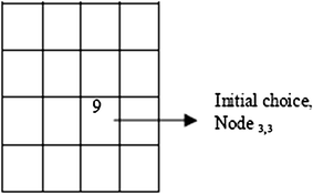
To illustrate this, the obtained topology of a 4 × 4 node matrix (for a desired total distance of 66 units) is shown in Fig. 3a–d. with ‘K’ chosen as 30. Hence N1 = [66–30] % 4 = 9. The Successive elements are formed with Δ c = 1 for that row.

Topology formation
3.1.1 Node Coverage
-
1.
Start from Node i,j = Node3,3 [Initial choice of i & j is arbitrary].
-
2.
Connect Node i,j with Nodep,k such that pk ≠ ij. Example i = j = 3 implies p and k cannot have this choice. Hence p = 2 and k = 4 i.e. Node2,4 is chosen as next choice.

-
3.
Repeat step (2) such that the new node satisfies both the conditions, ≠ ij & ≠ pk. This implies that
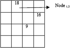


In this work, possible m,n values are constrained to m = 1, n = 1,2; m = 4, n = 1,2; Thus, m = 1 & n = 2 is chosen, then Nodep,k is connected with Node m,n i.e. Node2,4 is connected with Node1,2.
-
4.
Repeat (3) till only one node is left over. Possible values are m = 4, n = 1 (i.e.) element 23 in Fig. 3d.
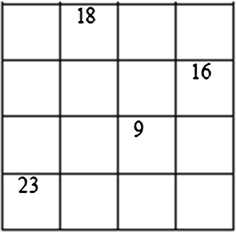

Node3,3 → Node2,4 → Node1,2 → Node4,1
Therefore, 9 + 16 + 18 + 23 = 66
The above nodes formation is not unique. The only Constraint is Nodei,j is connected with Nodep,k such that pk ≠ ij. The possible and non-existent paths are shown in Fig. 4.

Broadcast path formation. Initial Node 3, 3 to broadcast path. a Possible path, b Nonexistent path, c Possible path
Possible path–(Node3,3 → Node4,2 → Node2,1 → Node1,4)
-
a.
Nonexistent path–(Node3,3 → Node1,2 → Node2,1)
[Reason: Once Node1,2 is chosen the elements of 1st row and 2nd column are prohibited. Thus Node2,1 is non-existent since it includes element row = 1, column = 1 which is already included in Node1,2.]
-
b.
Possible path–(Node3,3 → Node1,4 → Node2,1 → Node4,2)
3.1.2 Adaptive Modulation and Path (Channel Behavior versus Modulation Type)
The objective is to maximize the SNR value and provide good channel.
-
Inputs: Distance between the nodes, IP address of the nodes, Channel support matrix.
-
User space: python ‘C’.
-
Implementation Steps: 1. Network Configuration 2. Data Transmission
-
1.
Network Configuration
-
1.
This implies node identification i.e. own node or source node
-
2.
All the channel parameters
-
3.
IP addresses assignment
-
4.
Open the UDP port (Packet size = 512 bytes) for communication in asynchronous mode
-
5.
Identify the total number of nodes in the network
-
1.
-
1.
-
Objective: To get the shortest path along with channel support.
-
Outputs: This includes sending Time, modulation Technique and modulated file size (logged in a file).
3.1.3 Data Transmission
The destination node is entered to receive the message. All possible paths from source to destination node and their corresponding weights depending on the channel parameters of each modulation technique is determined [12]. All possible clusters with their corresponding weights and the cluster that is also a shortest path to the destination is identified and the best cluster is chosen depending on the weight. The input data is modulated and sent over the best cluster path.
3.1.4 Receiving Message in Asynchronous Mode
If the received node is the destination node, the message is received else the message is forwarded to the next node depending on the best cluster path. After receiving the data, the data is demodulated [2]. If the data has to be forwarded, the demodulated data is again modulated and the modulated data is sent to the next node.
4 Experimental Setup
Four nodes were considered for study in this research and the network topology is shown in Fig. 5. With distance between the nodes indicated.

Network topology used for optimising the path from source to destination
The ip address for each node is configured and the distance between the 4 nodes is provided in the form of matrix as shown in Table 1.
Hardware implementation is done on FL2440 ARM Core with Linux OS customized kernel. Three methods of autonomous modulation detection were performed; one using the fixed, second using variable size headers (in deterministic) and finally using SVM classifier (in blind method). Generic cores are built using reconfigurable hardware for five popular modulation schemes. Using a microcontroller, the FPGA was programmed with respective bit files (configuration bits) and the modulation that had the best channel support is selected.
4.1 Implementation Details
For illustration, the source node is taken as 1 and destination node is 4 (refer Fig. 5). The different paths from 1 to 4 is identified as
The weights are determined as follows:
For the path 1–2–4 as example with two paths 1–2 and 2–4
The (1, 2) matrix values in all the channel parameters are illustrated in Table 1
From Table 2, the largest parameter value for path 1–2 is 0.9
Similarly, the (2, 4) matrix values in all the channel parameters are illustrated in Table 2.
From Table 2, the largest parameter value for path 2–4 is 0.8
The weights are calculated using a novel formula:
The path which yields maximum value is chosen. Thus, the weight for 1–2–4 is 0.9 × 100 + 0.8 × 100 = 170
Similarly, the weight for all the other paths is calculated as follows:
Using the shortest path algorithm, the shortest path is calculated from source node 1 to destination node 4 using the distance matrix is 1–4. For this link (1, 4), the matrix values in all the channel parameters are as shown in Table 2.
From Table 2, the largest parameter value for path 1–4 is 0.6
Therefore weight is 0.6 × 100 + 100 = 160
The best cluster chosen of all the paths with highest weight (i.e. 1–2–3–4) of 230 and accordingly the modulation type is chosen as given in Table 3.
To summarize,
-
For the path 1–2, 0.9 is highest, hence BASK modulation is determined as best suited.
-
For the path 2–3, 0.7 is highest; hence DQPSK modulation is determined as best suited.
-
For the path 3–4, 0.6 is highest; hence SUNDE modulation is determined as best suited
4.2 Simulated Output
Case (i)
Shortest path
The algorithm presented is implemented as a verilog core and tested for different combinations of source node and destination node. The simulated results for five nodes for the shortest path message transfer are given in Fig. 6.

Verilog simulated output illustrating the shortest path core [src node = 2, dst node = 5]
Case (ii)
Average bytes, average packets/s and jitter values.
The average bytes/s, average packes/s (Sent/received) and Jitter values for the packets forwarded to all the nodes (that support FTP applications) by the transport layer in the network is obtained using the OPNET simulation tool and results are plotted in Fig. 7a–d.

Average bytes per second a forwarded to all the nodes (bytes/s), b received by all the nodes (bytes/s), c submitted to all the nodes (bytes/s), d Time elapsed between sending a file and receiving the response to all the nodes
4.3 Inference from Results
Sl. no | Time | Traffic received (bytes/s) |
|---|---|---|
1. | 0 ms | 0 |
2. | 10 ms | 7,00,000 |
3. | 40 ms | 7,00,000 |
4. | 1 h | 0 |
Sl. no | Time | Traffic received (packets/s) |
|---|---|---|
1. | 0 ms | 0.027 |
2. | 10 ms | 0.027 |
3. | 40 ms | 0.027 |
4. | 1 h | 0 |
Sl. no | Time | Response time (s) |
|---|---|---|
1. | 0 ms | 0 |
2. | 10 ms | 56,345,475 |
3. | 40 ms | 56,345,475 |
4. | 1 h | 0 |
Sl. no | Time | Traffic received (packets/s) |
|---|---|---|
1. | 0 ms | 0.027 |
2. | 10 ms | 0.027 |
3. | 40 ms | 0.027 |
4. | 1 h | 0 |
5 Conclusion
Multiple hops introduced into a network can decrease the end to end delay in the reception of packets from source to destination, but, at the cost of increase in the number of nodes. This tradeoff is balanced in this work by choosing the shortest path through which the packets are routed among the selected nodes. Every node can modulate the incoming packet in an adaptive way depending on the data type and thus support hybrid data type (i.e. text, voice, video etc.). In this work, network that use channel state information either through feedback from the receiver to the transmitter or channel model using statistical approach is cooperatively used to allocate optimal transmit power, As the network is designed to guarantee uniform SNR good longevity of the network is ensured. Studied metrics include traffic received (packets/s), jitter, arrival rate and departure rate of packets (i.e. average packets/s received and submitted by a node) and response time (in s). Simulation study using OPNET simulator and implementation on FPGA hardware (using gnuradio cores built on linux platform) were demonstrated.
References
Ho, K. C., Prokopiw, W., & Chan, Y. T. (1995), Modulation identification by the wavelet transform. In Proceedings of the IEEE military communications conference (MILCOM’95), San Diego, CA (Vol. 2, pp. 886–890).
Ho, K. C., Prokopiw, W., & Chan, Y. T. (2000). Modulation identification of digital signals by the wavelet transform. IEE Proceedings, Radar, Sonar and Navig., 47, 169–176.
Rosti, A.-V., & Koivunen, V. (2000). Classification of MFSK modulated signals using the mean of complex envelope. In Proceedings of EUSIPCO-2000 (Vol. 1, pp. 581–584).
Nolan K. E., Doyle L., Mackenzie P., & O’Mahony, D. (2002). Modulation scheme classification for 4G software radio wireless networks. In Proceeding IASTED international conference on signal processing, pattern recognition and applications, pp. 25–31.
Guldemir, H., & Sengur, A. (2005). Proposed classification of analog modulated communication signals using clustering techniques: A Comparative Study. FÜ Fen ve Mühendislik Bilimleri Dergisi, 17(2), 247–256.
Hamid, E. Y. (2007). Automatic modulation classification of communication signals using wavelet transform. In Proceedings of the international conference on electrical engineering and informatics institute Teknologi bandung, Indonesia.
Dobre, O. A. (2007). Survey of automatic modulation classification techniques: classical approaches and new trends. Communications, IET, 1, 137–156.
He, T., & Zhou, Z.-O. (2008). Classification of modulated signals using multifractal features. Journal of the Chinese Institute of Engineers, 31(2), 335–338.
Wu, H.-C., Saquib, M., & Yun, Z. (2008). Novel automatic modulation classification using cumulant features for communications via multipath channels. IEEE Transactions on Wireless Communications, 7(8), 3098–3105.
Singh, C. K., Kumar, A., & Ameer, P. M. (2008). Performance evaluation of an IEEE 802.15.4 sensor network with a star topology. Wireless Networks, 14, 543–568.
Islam, M., Hannan, M. A., Samad, S. A., & Hussain, A. (2009). Modulation technique for software defined radio application. Australian Journal of Basic and Applied Sciences, 3(3), 1780–1785.
Ramkumar, B. (2009). Automatic modulation classification for cognitive radios using cyclic feature detection. Circuits and Systems Magazine, IEEE, 9, 27–45.
Hassan, Y., El-Tarhuni, M., & Assaleh, K. (2010), Comparison of linear and polynomial classifiers for co-operative cognitive radio networks. In IEEE 21st international symposium on personal indoor and mobile radio communications.
Faek, F. K. (2010). Digital modulation classification using wavelet transform and artificial neural network. Journal of ZankoySulaimani, 13(1), 59–70.
Aslam, M. W., Zhu, Z., & Nandi, A. K.(2010). Automatic digital modulation classification using genetic programming with K-nearest neighbor. In Military communications conference–unclassified program–waveforms and signal processing track.
Bagga, J., & Tripathi, N. (2011). Analysis of digitally modulated signals using instantaneous and stochastic features, for classification. International Journal of Soft Computing and Engineering (IJSCE), 1(2), 2231–2307.
Xiao, H., Shi, Y. Q., Su, W., & Kosinski, J. A. (2012). Support vector machine based automatic modulation classification for analog schemes. The Computing Science and Technology International Journal, 2(1), 44–49.
Borkotoky, S. S., Ellis, J. D., Juang, M. A., Kottapalli, S. L., & Pursley, M. B. (2013) New results on the performance of a protocol for adaptive modulation and coding. In IEEE military communications conference (pp. 1590–1592).
Thomas, Y. (2014) An efficient adaptive beamforming technique for operation in frequency-selective channels. National wireless research collaboration symposium (pp. 112–116).
Pao, W.-C., Chen, Y.-F., & Tsai, Meng-Gu. (2014). An adaptive allocation scheme in multiuser OFDM systems with time-varying channels. IEEE Transactions on Wireless Communications, 13(2), 669–679.
Wang, S., Zhou,N., Zhao, H., & Du, W. (2014) A cross-layer adaptive incremental cooperative relaying scheme for wireless sensor networks. In IEEE international conference on information and communications technologies 2014, pp. 1–6.
Franchi, N., Kloc, M., & Weigel, R. (2014) SDR-proved adaptive OFDM guard interval scheme for rapidly varying time-dispersive vehicular broadcast channels. In Wireless vehicular communications (WiVeC), IEEE 6th international symposium on 2014, pp. 1–5.
Zheng, K., Wang, Y., & Lei, L. (2010). Cross-layer queuing analysis on multihop relaying networks with adaptive modulation and coding. IET Communications, 4(3), 295–302.
Huang, W. L., & Letaief, K. B. (2007). Cross-layer scheduling and power control combined with adaptive modulation for wireless ad hoc networks. IEEE Transactions on Communications, 55(4), 728–739.
Dong, Y., & Chang, C. H. (2014). An improved autonomous cross-layer optimization framework for wireless multimedia communication. In Computer and information science (ICIS), IEEE/ACIS 13th international conference on 2014, pp. 53–58.
Repele, L., Muradore, R., Quaglia, D., & Fiorini, P. (2014). Improving performance of networked control systems by using adaptive buffering. IEEE Transactions on Industrial Electronics Society, 61(9), 4847–4856.
Dong, C., Yang, L. L., & Hanzo, L. (2015). Performance of buffer-aided adaptive modulation in multihop communications. IEEE Transactions on Communications, 63(10), 3537–3552.
Author information
Authors and Affiliations
Corresponding author
Appendix: Channel Parameters Matrix for 5 Modulation Techniques
Appendix: Channel Parameters Matrix for 5 Modulation Techniques
Link1 | Link2 | Link3 | Link4 | |
|---|---|---|---|---|
Channel parameter for BASK | ||||
Link1 | 0.0 | 0.9 | 0.1 | 0.6 |
Link2 | 0.9 | 0.0 | 0.6 | 0.8 |
Link3 | 0.1 | 0.6 | 0.0 | 0.7 |
Link4 | 0.6 | 0.8 | 0.7 | 0.0 |
Channel parameter for DQPSK | ||||
Link1 | 0.0 | 0.8 | 0.2 | 0.1 |
Link2 | 0.8 | 0.0 | 0.7 | 0.3 |
Link3 | 0.2 | 0.7 | 0.0 | 0.4 |
Link4 | 0.1 | 0.3 | 0.4 | 0.0 |
Channel parameter for 16QAM | ||||
Link1 | 0.0 | 0.6 | 0.2 | 0.3 |
Link2 | 0.6 | 0.0 | 0.1 | 0.1 |
Link3 | 0.2 | 0.1 | 0.0 | 0.4 |
Link4 | 0.3 | 0.1 | 0.4 | 0.0 |
Channel parameter for QASK | ||||
Link1 | 0.0 | 0.6 | 0.1 | 0.0 |
Link2 | 0.6 | 0.0 | 0.4 | 0.6 |
Link3 | 0.1 | 0.4 | 0.0 | 0.1 |
Link4 | 0.0 | 0.6 | 0.1 | 0.0 |
Channel parameter for SUNDE | ||||
Link1 | 0.0 | 0.2 | 0.4 | 0.1 |
Link2 | 0.2 | 0.0 | 0.1 | 0.2 |
Link3 | 0.4 | 0.1 | 0.0 | 0.6 |
Link4 | 0.1 | 0.2 | 0.6 | 0.0 |
Rights and permissions
Open Access This article is distributed under the terms of the Creative Commons Attribution 4.0 International License (http://creativecommons.org/licenses/by/4.0/), which permits unrestricted use, distribution, and reproduction in any medium, provided you give appropriate credit to the original author(s) and the source, provide a link to the Creative Commons license, and indicate if changes were made.
About this article

Cite this article
Navaneethan, C., Helen Prabha, K. Optimizing Network Layer with Adaptive Modulation for Time Varying Channel. Wireless Pers Commun 90, 1003–1019 (2016). https://doi.org/10.1007/s11277-016-3279-8
Published:
Issue Date:
DOI: https://doi.org/10.1007/s11277-016-3279-8