Correction: Spatio-Temporal Outdoor Lighting Aggregation on Image Sequences Using Transformer Networks

Correction: International Journal of Computer Vision https://doi.org/10.1007/s11263-022-01725-2

This erratum aims to correct errors in the sections 1, 3, and 5 of Lee et al. (2022). Some of the texts in these sections were reproduced in non-final form. It resulted in omissions of several major extensions that are made during the revision process. Figures and Tables are not affected.

1 1. Introduction

• The following sentence in the 3rd paragraph (Fig. 1) should be modified as:

  In our work, we go in a similar direction as we robustly estimate the global sun direction and other lighting parameters (Lalonde & Matthews, 2014) by fusing estimates both from the spatial and temporal domains.

  

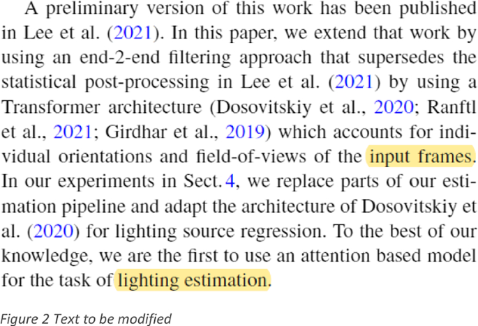
• The 5th paragraph (Fig. 2) should be modified as:

  … which accounts for individual orientations and field-of-views of the input frames. With this novel pipeline, we eliminate the necessity of intricate hyperparameter tuning required for post-processing. In our experiments in Sect. 4, we replace parts of our estimation pipeline and adapt the architecture of Dosovitskiy et al. (2020) for lighting source regression. To the best of our knowledge, we are the first to use an attention-based model for the task of lighting estimation. Finally, we extend our lighting model. Unlike previous work which predicted only the sun direction, the proposed work estimates parameters of the Lalonde-Matthews outdoor illumination model (Lalonde & Matthews, 2014).

  

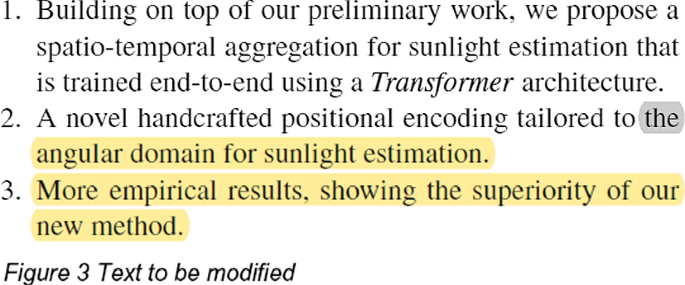
• The list of contributions in the 6th paragraph (Fig. 3) should be modified as:

  • 1. Building on top of our preliminary work, we propose a spatio-temporal aggregation for sunlight estimation that is trained end-to-end using a Transformer architecture.

  • 2. A novel handcrafted positional encoding tailored to encode the local and global camera angles for spatio-temporal aggregation.

  • 3. More realistic lighting estimation using the Lalonde-Matthews illumination model (Lalonde & Matthews, 2014).

  • 4. Superior performance compared to the state-of-the-art.

    

2 3. Proposed Method

• An additional sentence should be inserted after the last sentence of the 1st paragraph:

  In this way, the samples obtained from each sequence provide different observations for the same global lighting condition. This design is motivated by our empirical results, which showed that lighting can be estimated well from many small parts.

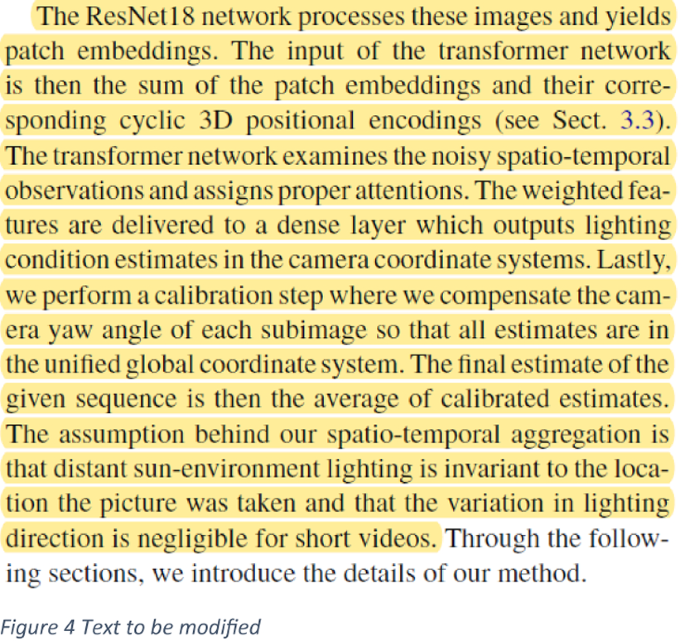
• The 2nd paragraph (Fig. 4) is completely rewritten as:

  All image crops are passed through the backbone network and projected to a sequence of patch embeddings. We then add an orientation-invariant positional encoding and pass the sequence to our transformer network. Through the attention layers, the noisy spatio-temporal observations can be effectively aggregated to a final estimate. Weighted features are delivered to a dense layer that produces the estimated Lalonde-Matthews illumination model parameters. The sun direction estimates are formulated in their own camera coordinate systems. We compensate the camera yaw angle of each subimage in order to obtain aligned estimates in a unified global coordinate system. Our final prediction is given as the average of all estimates. Note that the sky parameters of the Lalonde-Matthews model do not require the alignment step, as they do not vary with respect to the camera yaw angle. The assumption behind our spatio-temporal aggregation is that distant sun-environment lighting can be considered invariant for small-scale translations (e.g., driving) and that the variation in lighting direction is negligible for short videos. Through the following sections, we introduce the details of our method.

  

2.1 3.1 Lighting Estimation

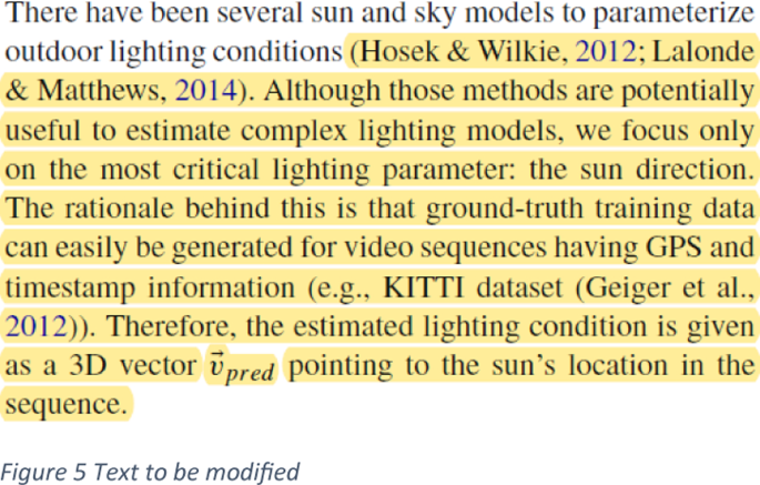
• The 1st paragraph (Fig. 5) is completely rewritten as:

  There have been several sun and sky models to parameterize outdoor lighting conditions such as the Hosek-Wilkie sky model (Hosek & Wilkie, 2012) or the Lalonde-Matthews (Lalonde & Matthews, 2014) outdoor illumination model. In this work, we extend our previous method by predicting the parameters of the Lalonde-Matthews model. This hemispherical illumination model (${f}_{LM}$) describes the luminance of outdoor illumination for a light direction $l$ as the sum of sun (${f}_{sun}$) and sky (${f}_{sky}$) components based on 11 parameters:

  $$ \begin{gathered} f_{LM} \left( {l;q_{LM} } \right) = {\varvec{w}}_{sun} f_{sun} \left( {l;{\upbeta },{\upkappa },l_{sun} } \right) + {\varvec{w}}_{sky} f_{sky} \left( {l;t,l_{sun} } \right), \hfill \\ f_{sun} \left( {l;{\upbeta },{\upkappa },l_{sun} } \right) = {\text{exp}}\left( { - {\upbeta }\,{\text{exp}}\left( { - \upkappa /{\text{cos}}\,{\upgamma }_{{\text{l}}} } \right)} \right), \hfill \\ f_{sky} \left( {l;t,l_{sun} } \right) = f_{P} \left( {{\uptheta }_{sun} ,{\upgamma }_{l} ,t} \right), \hfill \\ q_{LM} = \left\{ {{\varvec{w}}_{sun} ,{\varvec{w}}_{sky} ,{\upbeta },{\upkappa },t,{\varvec{l}}_{sun} } \right\}, \hfill \\ \end{gathered} $$

  where ${{\varvec{w}}}_{sun}\in {R}^{3}$ and ${{\varvec{w}}}_{sky}\in {R}^{3}$ are the mean sun and sky colors, ($\upbeta$, $\upkappa$) are the sun shape descriptors, $t$ is the sky turbidity, ${{\varvec{l}}}_{sun}=\left[{\uptheta }_{sun},{\upphi }_{sun}\right]$ is the sun position, ${\upgamma }_{l}$ is the angle between the light direction $l$ and the sun position ${l}_{sun}$, and ${f}_{P}$ is the Preetham sky model (Preetham et al., 1999). For more details, please refer to (Lalonde & Matthews, 2014).

  

• The following sentence should be inserted at the beginning of the 2^nd paragraph (Fig. 6):

  Among the parameters, the sun direction may be the most critical component. Unlike our predecessors …

  

  • The loss functions for the extended sun sky model should be attached at the end of Sect. 3.1 (below Eq. 4) as a new paragraph:

  For the remaining parameters, we apply the mean squared error (MSE) to the predicted values and the normalized ground truth values as in Jin et al. (2020):

  $${\mathrm{L}}_{{\mathrm{w}}_{\mathrm{sun}}}=\frac{1}{3}{\Vert {w}_{sun}^{pred}-{w}_{sun}^{gt}\Vert }_{2}^{2}$$
  $${L}_{{w}_{sky}}=\frac{1}{3}{\Vert {w}_{sky}^{pred}-{w}_{sky}^{gt}\Vert }_{2}^{2}$$
  $${L}_{beta}={\Vert {\beta }^{pred}-{\beta }^{gt}\Vert }_{2}^{2}$$
  $${L}_{kappa}={\Vert {\kappa }^{pred}-{\kappa }^{gt}\Vert }_{2}^{2}$$
  $${L}_{t}={\Vert {t}^{pred}-{t}^{gt}\Vert }_{2}^{2}$$
  $${L}_{param}=\frac{1}{5}\left[{L}_{{w}_{sun}}+{L}_{{w}_{sky}}+{L}_{beta}+{L}_{kappa}+{L}_{t}\right]$$

  Since the two loss functions ${L}_{sun}$ and ${L}_{param}$ have similar magnitudes, we define the final loss function as the sum of them:

  $${L}_{light}={L}_{sun}+{L}_{param}.$$

2.2 3.3 Orientation-Invariant Positional Encoding

• The occurrences of an abbreviation fov (field of view) in the 1st paragraph (Fig. 7) should be substituted with a spherical angle symbol ∢:

  For example, the top left pixel gets a coordinate of $\left(-\frac{{\sphericalangle }_{h}}{2},\frac{{\sphericalangle }_{v}}{2}\right)$ for a pinhole camera model with a field of view of ${\sphericalangle }_{h}$ and ${\sphericalangle }_{v}$ horizontally and vertically, respectively.

  

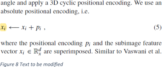
• The first occurrence of ${x}_{i}$ in the equation 5 (Fig. 8) should be substituted with ${x}_{i}^{enc}$:

  We use an absolute positional encoding, i.e.

  $${x}_{i}^{enc} \leftarrow {x}_{i}+{p}_{i,}$$

  where the positional encoding ${p}_{i}$ and the subimage feature vector ${\mathrm{x}}_{\mathrm{i}}\in {\mathbb{R}}_{x}^{d}$ are superimposed.

  

• The following sentence should be inserted after the last sentence:

  The resulting positional encoding of a subimage is the stacked vector of the three cyclic positional encodings. Note that the depth parameter d is carefully determined so that the depth of the stacked vector matches the channel size of the transformer network.

2.3 3.4 Calibration

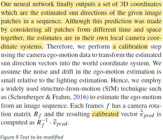
• Occurrences of ‘calibration’ and ‘calibrated’ should be substituted with ‘alignment’ and ‘aligned’. This change includes the subsection title.

• The first two sentences are completely rewritten to reflect the changes introduced by an extended sun and sky model.

• A new sentence is inserted at the end of the 1st paragraph. The correct text for these three changes is:

  3.4 Alignment

  Our neural network outputs the lighting parameters as a 11-dimensional vector for a given sequence of image patches. Although this prediction was made by considering patches from different temporal and spatial locations, the sun direction estimates are in their own local camera coordinate systems. Therefore, we perform an alignment step using the camera ego-motion data to transform the estimated sun direction vectors into the world coordinate system. We assume the noise and drift in the ego-motion estimation is small relative to the lighting estimation. Therefore, we employ a widely used structure-from-motion (SfM) technique such as Schonberger & Frahm (2016) to estimate the egomotion of an image sequence.

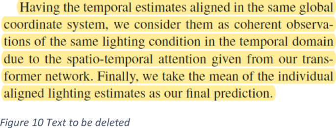
  Each frame $f$ has a camera rotation matrix ${R}_{f}$ and the resulting aligned vector ${\overrightarrow{v}}_{pred}$ is computed as ${R}_{f}^{-1}\cdot {\overrightarrow{v}}_{pred}$. Finally, we take the mean of the aligned lighting estimates as our final prediction.

  

• The second paragraph should be removed.

  

3 5. Conclusion

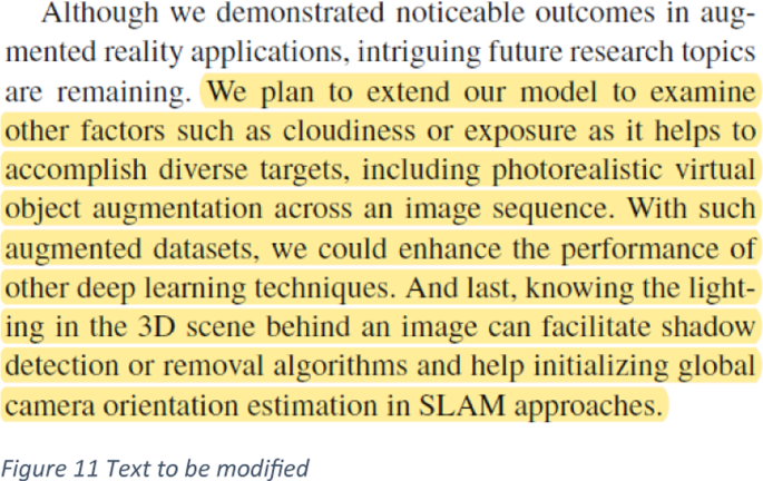
• The 2nd paragraph (Fig. 11) is completely rewritten as:

  Although we demonstrated visually appealing results in augmented reality applications, intriguing future research topics are remaining open. Intuitively, the performance of the model should scale with the sequence length, as more information is present. We plan to scale both our model and data to examine the limit of attention-based spatio-temporal aggregation for lighting estimation. Another interesting direction would be the integration of our method into reconstruction pipelines, such as SLAM. Knowing the lighting direction and shadow-casting can help initializing camera estimation. Lastly, we want to investigate further into the sampling methods. Instead of picking 8 random frames from an image sequence, we could think of selecting consecutive frames and experiment with the number of frames and the distance from the starting point.

References

Dosovitskiy, A., Beyer, L., Kolesnikov, A., Weissenborn, D., Zhai, X., Unterthiner, T., et al. (2020). An image is worth 16x16 words: Transformers for image recognition at scale. arXiv preprint arXiv:2010.11929.
Hosek, L., & Wilkie, A. (2012). An analytic model for full spectral sky-dome radiance. ACM Transactions on Graphics (TOG).
Jin, X., Deng, P., Li, X., Zhang, K., Li, X., Zhou, Q., et al. (2020). Sun-sky model estimation from outdoor images. Journal of Ambient Intelligence and Humanized Computing.
Lalonde, J.-F., & Matthews, I. (2014). Lighting estimation in outdoor image collections. IEEE International Conference on 3D Vision.
Preetham, A., Shirley, P., & Smits, B. (1999). A practical analytic model for daylight. In Proceedings of the 26th annual conference on Computer graphics and interactive techniques.
Schonberger, J., & Frahm, J.-M. (2016). Structure-from-motion revisited. In Proceedings of the IEEE conference on computer vision and pattern recognition.
Author information
Authors and Affiliations
Corresponding author
Additional information
Publisher's Note
Springer Nature remains neutral with regard to jurisdictional claims in published maps and institutional affiliations.
Rights and permissions
Open Access This article is licensed under a Creative Commons Attribution 4.0 International License, which permits use, sharing, adaptation, distribution and reproduction in any medium or format, as long as you give appropriate credit to the original author(s) and the source, provide a link to the Creative Commons licence, and indicate if changes were made. The images or other third party material in this article are included in the article's Creative Commons licence, unless indicated otherwise in a credit line to the material. If material is not included in the article's Creative Commons licence and your intended use is not permitted by statutory regulation or exceeds the permitted use, you will need to obtain permission directly from the copyright holder. To view a copy of this licence, visit http://creativecommons.org/licenses/by/4.0/.
About this article
Cite this article
Lee, H., Homeyer, C., Herzog, R. et al. Correction: Spatio-Temporal Outdoor Lighting Aggregation on Image Sequences Using Transformer Networks. Int J Comput Vis 131, 1302–1306 (2023). https://doi.org/10.1007/s11263-022-01747-w
Accepted:
Published:
Issue Date:
DOI: https://doi.org/10.1007/s11263-022-01747-w